Behrens: Department of Economics, Université du Québec à Montréal (UQAM) and CIRPÉE, Canada; CEPR, UK [email protected]
Murata: Advanced Research Institute for the Sciences and Humanities (ARISH), Nihon University, 12-5, Goban-cho, Chiyoda-ku, Tokyo 102-8251, Japan; and Nihon University Population Research Institute (NUPRI), Japan
Cahier de recherche/Working Paper 09-28
Globalization and Individual Gains from Trade
Kristian Behrens Yasusada Murata
Abstract:
We analyze the impact of globalization on individual gains from trade in a general equilibrium model of monopolistic competition featuring product diversity, pro-competitive effects and income heterogeneity between and within countries. We show that, although trade reduces markups in both countries, its impact on variety depends on their relative position in the world income distribution: product diversity in the lower income country always expands, while that in the higher income country may shrink. When the latter occurs, the richer consumers in the higher income country may lose from trade because the relative importance of variety versus quantity increases with income. We illustrate this effect using data on GDP per capita and population for 186 countries, as well as parameter estimates for domestic income distributions. Our results suggest that U.S. trade with countries of similar GDP per capita makes all agents in both countries better off, whereas trade with countries having lower GDP per capita may adversely affect up to 11% of the U.S. population.
Keywords: Income heterogeneity, product diversity, pro-competitive effects, general
equilibrium, monopolistic competition
1
Introduction
The questions of whether there are gains from trade and how these gains are distributed are two of the oldest, and most fundamental ones, in international economics. As is well known, trade alters the distribution of income across some broad ‘classes’ such as workers and the owners of capital (Jones, 1965). Trade also adversely affects the owners of resources that are specific to import-competing sectors (Jones, 1971). While it is, therefore, possible that trade hurts particular groups, the fundamental insight advocated by economists is that, under the assumption of perfect markets, the nation as a whole unambiguously gains. Such gains from trade at the aggregate level have also been largely confirmed under imperfect competition where product diversity and scale economies matter (Helpman and Krugman, 1985, Ch.9).1
Do these aggregate gains from trade, which theoretically make possible a Pareto-improving redistribution, constitute a relevant welfare criterion for globalization? The answer is likely to be negative. Globalization, as Stiglitz (2006, p.63) puts it, “only promises that the country as a whole will benefit. Theory predicts that there will be losers. In principle, the winners could compensate the losers; in practice, this almost never happens.” Given that compensation mechanisms are unlikely to be operational, gains from trade should be assessed at the individual
level. The relevant criterion is then whether aggregating individual preferences for trade, not
aggregating individual gains, leads to globalization. The answer clearly depends on the fraction of agents who gain from trade, irrespective of the magnitude of aggregate gains.
We explore the impact of globalization on individual gains from trade in a general equilib-rium model of monopolistic competition building on Behrens and Murata (2007). There are two crucial ingredients in the model. First, we consider that workers are heterogeneous in terms of labor efficiency and, therefore, in terms of income, both between and within countries. Second, we focus on a variable elasticity of substitution (VES) case because, unlike in the constant elasticity of substitution (CES) case, the relative importance of variety versus quantity changes with income. Within such a framework, individual gains from trade can be decomposed into those due to product diversity and those due to pro-competitive effects. In order to focus en-tirely on these two aspects, we abstract from comparative advantage and income distribution across factors by considering a setting with a single production factor.
Our main results may be summarized as follows. First, in the presence of income hetero-geneity between countries, the impact of trade on variety depends on their relative position in the world income distribution. In the lower income country, product diversity in consumption always expands, whereas it may shrink in the higher income country. Second, trade always reduces markups in both countries.2 Consequently, all individuals in the lower income country 1Helpman and Krugman (1985) derive the general result that there are gains from trade: (i) when free trade
income and prices enable the economy to purchase autarky aggregate consumption quantities; and (ii) when switching from autarky to free trade expands product diversity in consumption.
always gain from trade because of lower markups and greater product diversity in consumption. Turning to the higher income country, two cases may arise. First, when its trading partner has sufficiently similar average income, the range of varieties expands and markups fall, thus benefiting all consumers. Second, when its trading partner has sufficiently lower average in-come, the range of varieties shrinks, while markups fall. In the latter case, whether individuals in the higher income country gain or not depends on their position in the domestic income
distribution.
We show that it is the richer consumers in the higher income country who may lose from trade because the relative importance of variety versus quantity increases with income. The intuition is that since utility is bounded for each variety in our framework, the richer consumers benefit only little from increased quantity due to a fall in the price-wage ratios, whereas a decrease in product diversity hurts them. On the contrary, lower income consumers care less about variety but more about quantity, and they gain from trade even when facing less product diversity because the lower price-wage ratios allow them to consume more of each variety. Our result thus suggests that measured income inequality under a trade regime may overstate ‘real’ inequality, as the former neglects the different trade-offs between variety and quantity faced by high and low income consumers. This is reminiscent of recent work by Broda and Romalis (2009), who show that much of the rise in measured U.S. income inequality is offset by a relative decline in the prices of products that low income consumers buy.
We finally illustrate how many individuals in the higher income country are likely to lose from trade. Using data on GDP per capita and population for 186 countries, as well as param-eter estimates for domestic income distributions, we show that U.S. intra-industry trade with countries of similar GDP per capita makes all agents in both countries better off, whereas U.S. intra-industry trade with countries having lower GDP per capita may adversely affect up to 11% of the U.S. population.3
The remainder of the paper is organized as follows. Section 2 briefly reviews the related lit-erature. Section 3 presents the model and derives the equilibrium conditions. Section 4 focuses on the case of homogeneous populations within each country. This allows to build intuition for a more general case of heterogeneous populations between and within countries. Section 5 analyzes the general case and provides some numerical illustrations. Section 6 concludes.
opposite effects on markups. First, the variety loss under free trade reduces competition, thus raising markups. Second, firms in the higher income country face lower average income under free trade than in autarky, which makes demand more elastic, thus reducing markups. The latter effect always dominates the former in our framework, so that markups fall when switching from autarky to trade.
3One may think of relatively new OECD member countries. Indeed, recent work by the OECD (2002,
p.161) classifies Czech Republic, Slovak Republic, Mexico, Hungary and Germany, the United States, Poland as countries with “high and increasing intra-industry trade”. This suggests that the set of countries with high intra-industry trade is becoming more dissimilar in terms of GDP per capita.
2
Related literature
Recent empirical research in international trade has substantiated the importance of product diversity and pro-competitive effects. Using extremely disaggregated data, Broda and Weinstein (2006) document that the number of U.S. import varieties rose by 212% between 1972 and 2001, which maps into U.S. welfare gains of about 2.6%. Badinger (2007) finds solid evidence that the Single Market Programme of the EU has reduced markups by 26% in aggregate manufacturing of 10 member states. See also Levinsohn (1993), Harrison (1994) and Tybout (2003) for earlier empirical evidence on pro-competitive effects of international trade.
Despite such empirical evidence, theoretical research has not explored how individual wel-fare is affected by the relative importance of product diversity and pro-competitive effects. Instead, the seminal work by Mayer (1984), for instance, analyzes how the difference in capital endowments across individuals maps into individual preferences for trade openness via changes in factor prices as implied by the Stolper-Samuelson theorem. This prediction under perfect competition has been recently examined and confirmed by using individual survey data (e.g., Balistreri, 1997; Scheve and Slaughter, 2001; Hamilton, 2004; Mayda and Rodrik, 2005).
On the contrary, the monopolistic competition literature focuses either or both on prod-uct diversity and pro-competitive effects, without taking into account income heterogeneity (Krugman 1979, 1980). One notable exception is Krugman (1981) who considers a two-factor two-sector monopolistic competition model without intersectoral factor mobility. Since coun-tries differ in relative factor endowments, not only product diversity but also factor prices determine whether each factor gains or not. However, there is no income heterogeneity within each factor and pro-competitive effects do not arise due to the constant elasticity specification. In this paper, we show that when income heterogeneity and variable demand elasticity are jointly taken into account, trade may reduce product diversity in consumption.4 This has
important welfare implications because individual gains from trade depend on product diversity and pro-competitive effects. Saint-Paul (2006) also uses a variable elasticity model and analyzes the impact of globalization on wages when the total mass of firms is exogenously given and when there is no income heterogeneity within each country. Since our model allows for free entry and exit and income heterogeneity both between and within countries, we can analyze more precisely how the relative importance of variety and quantity affects individual welfare.
Finally, Flam and Helpman (1987) and Stokey (1991) consider the relative importance of quality and quantity. Although this literature on vertical product differentiation essentially deals with the patterns of consumption and specialization, we investigate the impact of trade on individual welfare in the presence of income heterogeneity between and within countries. The related paper by Matsuyama (2000) puts more emphasis on demand complementarities and multisectoral issues under perfect competition, whereas we focus on individual gains from
4Note that this possibility arises even when the number of import varieties increases because the number of
trade through product diversity and pro-competitive effects under monopolistic competition.
3
Model
Consider a world with two countries, labeled r = H, F . Variables associated with each country will be subscripted accordingly.5 Each country is endowed with a mass L
r of population. Let
L≡ LH+ LF denote the world population, and let θ ≡ LH/L stand for the population share of country H. We assume that labor is the only factor of production and that it is internationally immobile. Furthermore, the labor efficiency may differ both between and within countries. We denote by Gr the cumulative distribution function and by gr the density function of labor efficiency in country r. Both are assumed to be continuously differentiable, with support [0,∞). An individual with labor efficiency hr supplies inelastically that many units of labor. The aggregate labor supply in country r is then given by Lrhr, where hr ≡
R
hrdGr(hr) is the average labor efficiency in that country.
3.1
Preferences
There is a single monopolistically competitive industry producing a continuum of varieties of a horizontally differentiated consumption good. Let Ωr denote the set of varieties produced in country r, with measure nr. Hence, N ≡ nr + ns stands for the endogenously determined mass of varieties in the global economy. Following Behrens and Murata (2007), we assume that preferences are additively separable over varieties and that the subutility functions are of the ‘constant absolute risk aversion’ (CARA) type:
max Ur ≡ Z Ωr £ 1− e−αqrr(i)¤di + Z Ωs £ 1− e−αqsr(j)¤dj s.t. Z Ωr pr(i)qrr(i)di + Z Ωs ps(j)qsr(j)dj = Er(hr),
where pr(i) and ps(j) stand for the prices of varieties i and j produced in countries r and s;6
qrr(i) and qsr(j) stand for the consumption of domestic and foreign varieties in country r;
Er(hr) stands for expenditure; and α > 0 is a parameter. The individual with labor efficiency
hr spends Er(hr) ≡ wrhr+ Π/L, where wr stands for the wage rate in country r and Π/L stands for the identical claim to aggregate profits across individuals.7
5To reduce the notational burden, we present a two-country version of the model. However, the model can
be extended to an arbitrary number of countries without qualitatively affecting our results.
6We assume that there are no impediments to trade and that product markets are integrated, i.e., firms
cannot price discriminate across markets. This explains why there is only a single subscript for prices.
7Since our focus is not on the sources of income heterogeneity, we assume that it is solely driven by the
difference in labor efficiency, not by the difference in profit claims. The assumption of equal profit claims entails no loss of generality as each firm is negligible and earns zero profit in equilibrium under free entry and exit.
As shown in Appendix A, the demand functions in country r at an interior solution are given as follows: qrr(i, hr) = Er(hr) P − 1 αP ½Z Ωr ln · pr(i) pr(j) ¸ pr(j)dj + Z Ωs ln · pr(i) ps(j) ¸ ps(j)dj ¾ , (1) qsr(j, hr) = Er(hr) P − 1 αP ½Z Ωr ln · ps(j) pr(i) ¸ pr(i)di + Z Ωs ln · ps(j) ps(i) ¸ ps(i)di ¾ , (2) where P ≡ RΩ rpr(k)dk + R
Ωsps(k)dk. Because marginal utility at zero consumption is finite,
demands need not be strictly positive in equilibrium. In Section 3.3.2, we derive a sufficient condition for the price equilibrium to be symmetric, which then makes sure that (1) and (2) hold since the solution will be interior.
Finally, because of the continuum assumption, changes in an individual price have no impact on the price aggregates, so that the own-price derivatives are as follows:
∂qrr(i, hr) ∂pr(i) =− 1 αpr(i) and ∂qsr(j, hr) ∂ps(j) =− 1 αps(j) . (3)
3.2
Technology
All firms have access to the same increasing returns to scale technology. To produce Q(i) units of any variety requires cQ(i) + f units of labor, where c and f denote the marginal and the fixed labor requirements, respectively. We assume that firms can costlessly differentiate their products and that there are no scope economies. Thus, there is a one-to-one correspondence between firms and varieties, so that the mass of varieties N also stands for the mass of firms operating in the global economy. There is free entry and exit in each country, which implies that nr and ns are endogenously determined by the zero profit conditions. The profit of firm i in country r is given by:
Πr(i) = [pr(i)− cwr] Qr(i)− fwr, (4) where Qr(i)≡ Lr
R
qrr(i, hr)dGr(hr) + Ls R
qrs(i, hs)dGs(hs) stands for its output.
3.3
Equilibrium
3.3.1 Definition
Each firm in country r maximizes its profit (4) with respect to pr(i), taking the couples (nH, nF) and (wH, wF) of firm distributions and factor prices as given. Rearranging terms, the first-order conditions can be expressed as follows:
∂Πr(i) ∂pr(i) = Qr(i)− L [pr(i)− cwr] αpr(i) = 0. (5)
Expression (5) highlights a fundamental property of monopolistic competition: although each firm is negligible to the market, it must take into account the pricing decisions of the other
firms since the price aggregates affect its first-order condition. A price equilibrium is a price distribution satisfying condition (5) for all firms in countries H and F . An equilibrium is a price equilibrium and couples (nH, nF) and (wH, wF) of a firm distribution and factor prices such that national factor markets clear, trade is balanced, and firms earn zero profits. Formally, an equilibrium is a solution to the following three conditions:
Z ΩH £ cQH(i) + f ¤ di = LH Z hHdGH(hH), (6) Z ΩF £ cQF(j) + f ¤ dj = LF Z hFdGF(hF), (7) LH Z Z ΩF pF(j)qF H(j, hH)djdGH(hH) = LF Z Z ΩH
pH(i)qHF(i, hF)didGF(hF), (8) where all quantities are evaluated at a price equilibrium. One may set either wH or wF as the numeraire. However, we need not do so since the model is fully determined in real terms.8
Finally, it can be readily verified that firms earn zero profits when conditions (6)–(8) hold. Hence, aggregate profits are zero and the expenditure of an individual with labor efficiency hr is solely given by wage income: Er(hr) = wrhr.
3.3.2 Properties
In general equilibrium models of imperfect competition, the existence, the uniqueness, and the properties of the price equilibria are usually difficult to establish. The reason is that when firms have an influence on market aggregates, reaction functions can be badly behaved (Roberts and Sonnenschein, 1977). This problem does not occur in continuum models of monopolistic competition because firms have no influence on market aggregates.9 However, two additional
questions arise in our open economy model with income heterogeneity and finite marginal utility at zero consumption: (i) under which conditions the price equilibrium is symmetric; and (ii) under which conditions product and factor prices are equalized under free trade. Note that the answers to these questions are not trivial. Indeed, some firms may find it profitable to deviate from symmetric pricing by charging higher prices to higher income consumers while excluding lower income consumers. Furthermore, firms sell differentiated varieties, so that product price equalization (PPE) and factor price equalization (FPE) need not hold under free trade, even if many studies assume, rather than prove, that this is the case.
In what follows, we first show that free trade leads to both PPE and FPE provided each individual consumes all varieties. We then derive a sufficient condition for this to hold.
8The choice of the numeraire is immaterial in our monopolistic competition framework. This is an important
departure from general equilibrium oligopoly models, where the choice of the numeraire is not always neutral (Gabszewicz and Vial, 1972).
9In a similar spirit, to ensure the existence of a general equilibrium under oligopolistic competition, Neary
(2003) considers a model with a continuum of sectors, in which firms are large in their own sector but negligible in the whole economy.
Proposition 1 Assume that each individual consumes all varieties. Then, free trade leads to product and factor price equalization. Furthermore, the product price is uniquely given by
p = cw + αE N where E ≡ θ Z EH(hH)dGH(hH) + (1− θ) Z EF(hF)dGF(hF). (9)
Proof. See Appendix B.
As can be seen from (9), there are pro-competitive effects, i.e., the profit-maximizing price is decreasing in the mass of competing firms. Furthermore, it is increasing in the average expenditure E.10 Since FPE implies that E = wh, where h ≡ θh
H + (1− θ)hF denotes the world average labor efficiency, the product price can be rewritten as
p = µ 1 + αh cN ¶ cw. (10)
So far, we have assumed that each individual consumes all varieties. However, in the presence of income heterogeneity and finite marginal utility at zero consumption, some firms may find it profitable to deviate from the symmetric price by charging higher prices to higher income consumers while excluding lower income consumers. We now derive a sufficient condition under which there is no such incentive to unilaterally deviate from (9).
Proposition 2 Let ep stand for the price charged by a firm which is unilaterally deviating from the symmetric price (9). A sufficient condition for (9) to be a price equilibrium, i.e., for such a unilateral deviation to be unprofitable, is that
θRh∞l(ep)hH dGH(hH) + (1− θ) R∞ hl(p)ehF dGF(hF) θRh∞l(p)e dGH(hH) + (1− θ) R∞ hl(p)e dGF(hF) ≤ hl (ep) + h + c αU (h l (ep)), ∀ep > p, (11) where hl(ep) ≡ max ½ 0, N p αwln µ ep p ¶¾ . (12)
is the labor efficiency of the marginal consumer. Proof. See Appendix C.
We assume that the sufficient condition (11), which states that the average income of those who consume the variety must not rise too fast, holds throughout the paper. Note that it is never profitable to deviate from the symmetric price by charging lower prices (ep < p) because such a deviation does not affect the mass of consumers with positive demand, as can be seen
10Using “0/1 preferences”, Foellmi et al. (2008) also obtain a similar product price when labor efficiency
differs between countries but population sizes are the same. Note, however, that our product price depends both on income heterogeneity and on population shares. By contrast, the product price in Foellmi et al. (2008) includes trade costs. See Behrens et al. (2009) for how trade costs affect the product price in the CARA specification with heterogeneous firms.
from (12). In that case, p, as given by (9), is the unique profit-maximizing price. Note finally that FPE is compatible with income heterogeneity between and within countries because of the difference in labor efficiency. Hence, without loss of generality, we can restrict ourselves to the case in which FPE holds since our aim is to analyze the impact of trade on individual welfare in the presence of income heterogeneity, with less emphasis on the sources of this heterogeneity.
4
Homogeneous populations within each country
We first present the simple case in which all individuals within each country have the same labor efficiency. Without loss of generality, we assume that the labor efficiency in country H is higher than or equal to that in country F , i.e., hH ≥ hF.
4.1
Autarky
Assume that country r is in autarky (formally, Ωs =∅ and Ls = 0). As shown by Behrens and Murata (2007), the price equilibrium without income heterogeneity is symmetric, which allows to alleviate notation by dropping the variety index i. Inserting (1) into (5), and letting qrs= 0, the unique price equilibrium is given by:
par = µ 1 + αhr cna r ¶ cwar, (13)
where an a-superscript denotes autarky values. Note that (13) is a special case of the symmetric price equilibrium (10).
The symmetric price equilibrium implies that the budget constraint can then be rewritten as
qa
r = (warhr)/(narpar), which, when inserted into the labor market clearing condition (6), yields:
nar = Lrhr f µ 1−cw a r pa r ¶ . (14)
Expressions (13) and (14) allow us to solve for the equilibrium mass of firms as follows:11
nar = hrD(Lr) where D(Lr)≡ p
4αcf Lr+ (αf )2− αf
2cf > 0. (15)
It is readily verified that na
r is increasing in hr for any given value of Lrhr. Put differently, in autarky, a higher average labor efficiency hr maps into greater product diversity for any given aggregate labor supply Lrhr. The intuition is that an increase in hr makes demands less elastic, because consumers are richer and thus less price sensitive. As can be seen from (13), this raises markups, thus leading to entry and to the production of more varieties.
4.2
Free trade
We now analyze the impact of globalization on welfare when populations are homogeneous within each country. To do so, we first restate the sufficient condition for the symmetric price equilibrium (11) and derive the equilibrium under free trade. As shown in Appendix C, a unilateral deviation is possibly profitable only when the firm can affect the marginal consumer. Since the density function has a point-mass at hr when populations are homogeneous within each country, the mass of individuals with positive demand changes at hF and hH. Because
hF ≤ hH by assumption, three cases may arise: (i) hl(ep) ∈ (0, hF), where all consumers have positive demand; (ii) hl(ep) ∈ [hF, hH), where only consumers in country H have positive demand; and (iii) hl(ep) ∈ [hH,∞), where no consumer has positive demand.
Obviously, there is no incentive for the firm to deviate from the symmetric price p to the prices corresponding to cases (i) and (iii). This is because the deviating firm cannot change the mass of consumers it faces in case (i), whereas in case (iii) it faces zero demand. In what follows, we thus focus on case (ii).12 Because the demand functions are differentiable with
respect to ep when hl(ep) ∈ [h
F, hH), the sufficient condition for a symmetric price equilibrium given in Proposition 2 can be rewritten as:
hH ≤ hl(ep) + h +
c αU (h
l(ep)) ∀ep such that hl(ep) ∈ [h
F, hH). (16)
When condition (16) holds, which we previously assumed to be the case, Proposition 1 implies that the price equilibrium is symmetric and given by (10). Because prices and wages are equalized, all firms sell the same quantity Q = (LHhH+ LFhF)(w/N p). Labor market clearing then implies that nH/nF = (LHhH)/(LFhF), which yields
nr = Lrhr f µ 1− cw p ¶ , (17)
Inserting (10) into (17), and doing the same with the analogous expressions for s 6= r, we obtain two equations with two unknowns nH and nF (recall that N ≡ nH + nF). Solving for the equilibrium masses of firms, we readily obtain
nH = θhHD(L) and nF = (1− θ)hFD(L). The equilibrium mass of firms in the global economy is then given by
N ≡ nH + nF = hD(L). (18)
Comparing expressions (14) and (17), we see that nr < nar if and only if the free trade price-wage ratio is smaller than the autarky price-price-wage ratio. We show that this is always the case, as in Krugman (1979) and Feenstra (2004). Interestingly, unlike in the existing literature without income heterogeneity between countries, we further show that product diversity in
12Note that case (ii) does not arise when h
consumption may not expand for all individuals when switching from autarky to trade. The following proposition summarizes the results.
Proposition 3 Assume that the labor efficiency in country H is greater than or equal to that in country F , i.e., hH ≥ hF. When compared with autarky, we show that under free trade: (i)
the mass of varieties consumed in country H decreases if and only if
hHD(LH) > hD(L), (19)
whereas that in country F always increases; (ii) the mass of varieties produced in each country decreases; and (iii) the price-wage ratio falls in each country.
Proof. Since by assumption hF ≤ h ≤ hH and max{LH, LF} < L, expressions (15) and (18) reveal that N > na
F, whereas N T naH if and only if hHD(LH)S hD(L), which establishes (i). Comparing (10) and (13) establishes (iii) because (15) and (18) imply hr/nar > h/N for r =
H, F . By (14) and (17), this implies that nr < nar for r = H, F , thus proving (ii).
It is worth noting that variable elasticity and income heterogeneity between countries are crucial for our results. Baldwin and Forslid (2006) and Arkolakis et al. (2008) obtain a similar variety loss in CES models with firm heterogeneity. However, welfare implications of our variety loss are quite different from theirs. As we show in Section 5, welfare decreases for a subset of consumers in our model because, unlike in their CES models, the relative importance of variety versus quantity changes with income. On the contrary, Baldwin and Forslid (2006) and Arkolakis et
al. (2008) show that welfare rises even when there is a variety loss.
Some comments are in order. First, one may ask whether there always exists hH satisfying both (16) and (19). To check this, note that the sufficient condition (16) is satisfied when
1≤ hH
hF
≤ 2− θ
1− θ ≡ Φ(θ),
where we use the more stringent condition hH ≤ hF + h < hl(ep) + h + (c/α)U(hl(ep)) for all ep such that hl(ep) ∈ [hF, hH). Expression (19), in turn, requires that
hH
hF
> (1− θ)D(L)
D(θL)− θD(L) ≡ Ψ(θ).
Noting that limθ→0Φ(θ) = 2, limθ→1Φ(θ) = ∞, limθ→0Ψ(θ) = ∞, limθ→1Ψ(θ) = 2 + [α +
cD(L)]f /cL, and that Φ is increasing whereas Ψ is decreasing in θ∈ [0, 1], Φ and Ψ cross only
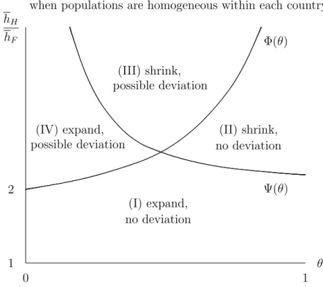
once for θ ∈ [0, 1].13 Based on these observations, the four possible cases are summarized in Figure 1.
Insert Figure 1 about here.
13Note that Ψ is decreasing in θ∈ [0, 1] because Ψ is convex and lim
Case (I) in Figure 1 shows that when hH/hF is sufficiently small, no firm wants to deviate, and hence, PPE and FPE hold. Furthermore, product diversity expands in both countries under free trade irrespective of the value of θ. More interestingly, case (II) shows that there exists couples (θ, hH/hF) such that no firm wants to deviate, and hence, PPE and FPE hold; whereas product diversity in consumption shrinks in the higher income country when switching from autarky to trade. This may make consumers in the higher income country worse off, depending on the relative importance of product diversity and pro-competitive effects. In cases (III) and (IV), when hH/hF is large enough, the sufficient condition for no deviation is not satisfied and hence PPE and FPE may not hold. Hence, the results on whether product diversity expands or not should be interpreted cautiously in these cases.
Second, Proposition 3 illustrates exit of firms due to the pro-competitive effects of interna-tional trade. As can be seen from the equilibrium price-wage ratios
pa r wa r = c + α D(Lr) and p w = c + α D(L), (20)
the equilibrium markups in both countries decrease under free trade, thus driving some firms out of each national market.14 Labor market clearing then implies that firm-level and total
production expands, as labor is reallocated from the fixed requirements of closing firms to the marginal requirements of surviving firms. Contrary to the growing literature on firm het-erogeneity in international trade (e.g., Melitz, 2003), where the price-cost margin is usually constant because of the CES specification, our model captures the ‘old idea’ that international trade reduces markups and hence triggers exit of firms even without firm heterogeneity.15
Last, one can readily verified that
∂nr ∂Lr > 0, ∂ns ∂Lr < 0, ∂nr ∂hr > 0 and ∂ns ∂hr = 0 for r 6= s.
Interestingly, an increase in population in country r reduces the mass of firms in country s, whereas an increase in average labor efficiency has no such impact. This is because there are both direct and indirect effects, as can be seen from (17). First, increases in population and average labor efficiency directly raise the domestic aggregate labor supply, thus increasing the mass of domestic firms. Second, an increase in population in country r has a negative effect on the equilibrium markups (20) and, therefore, reduces indirectly the equilibrium mass of firms in
14In Lawrence and Spiller (1983, Proposition 7), trade leads to a redistribution of firms between the two
countries while the total mass of firms remains unchanged. This result is driven by changes in relative factor prices and, as pointed out by the authors, need not hold under variable markups. Furthermore, they show in Proposition 5 that the price of the monopolistically competitive good falls in one country and rises in the other due to changes in relative factor prices. Yet, the markups remain constant because of the CES specification.
15One notable exception is Melitz and Ottaviano (2008) who recently proposed a model that explains
trade-induced exit by combining pro-competitive effects and firm heterogeneity in a monopolistic competition frame-work. However, due to their quasi-linear specification, there is no point in introducing income heterogeneity in their model as higher income consumers would spend their additional income only on the numeraire good.
both countries, whereas an increase in average labor efficiency has no impact on the equilibrium markups.
4.3
Welfare decomposition and gains from trade
We analyze gains from trade by decomposing welfare changes into those due to product diversity and those due to pro-competitive effects. Since the price equilibrium is symmetric under both autarky and free trade, we have qa= (wrahr)/(narpar) and q = (whr)/(N p). The utility difference between free trade and autarky in country r = H, F can then be expressed as follows:
∆Ur(hr)≡ Ur(hr)− Ura(hr) = N ³ 1− e−αwhrN p ´ − na r µ 1− e− αwar hr nar par ¶ .
Adding and subtracting nare−αwhr/(narp) and rearranging, we obtain the following decomposition:
∆Ur(hr)≡ N ³ 1− e−αwhrN p ´ − na r ³ 1− e−αwhrnar p ´ | {z } Product diversity + nar ³ e− αwar hr nar par − e− αwhr nar p ´ | {z } Pro-competitive effects , (21)
which isolates the two channels, namely product diversity and pro-competitive effects, through which gains from trade materialize. The former captures welfare changes through product diversity given the wage-price ratio under free trade w/p, whereas the latter captures welfare changes through the wage-price ratio given product diversity under autarky na
r.
Using the results of Proposition 3 and the welfare decomposition (21), we first consider the benchmark case in which populations are homogeneous even between countries. Noting that expression (19) never holds when hH = hF, we can show the following proposition.
Proposition 4 Assume that the two countries have the same average labor efficiency, i.e., hH = hF = h. Then, free trade raises welfare through greater product diversity in consumption
and through lower price-wage ratios.
Proof. Proposition 3 shows that when hH = hF = h, trade always expands product diversity in consumption, which raises welfare via ‘love-of-variety’ as follows. Given the price-wage ratio under free trade, we have Ur = N [1− e−αwh/(Np)] and ∂Ur/∂N = 1− e−αwh/(Np)[1 +
αwh/(N p)] > 0 for all N and r = H, F . To obtain the last inequality, let z ≡ αwh/(Np) and ξ(z) ≡ 1 − e−z(1 + z). Clearly, ξ(0) = 0 and ξ0(z) > 0 for all z > 0, which shows that for any given price-wage ratio under free trade, utility increases in the mass of varieties consumed. Hence, the first term in (21) is positive. Similarly, by Proposition 3, we know that for any given mass of firms under autarky, the price-wage ratio falls under free trade, thus implying that the second term in (21) is also positive.
On the contrary, the mass of varieties consumed in country H may decrease when hH > hF, as can be seen from Proposition 3. More specifically, when θ and hH/hF belong to (II) in
Figure 1, the first term in (21) is no longer positive. When this occurs, there may be losses from trade in the higher income country despite a fall in the price-wage ratios. In what follows, we explore this possibility by analyzing a more general case in which populations are heterogeneous both between and within countries.
5
Heterogeneous populations between and within
coun-tries
So far, we have shown that whenever there is a variety loss in the presence of income hetero-geneity between countries, it occurs in the higher income country. We now analyze who in the
higher income country may lose from trade by exploring gains from trade at the individual
level.
5.1
Welfare decomposition and gains from trade
Unlike in the previous section where all individuals in a country are affected in the same way by trade, income heterogeneity within a country matters when assessing who gains and who loses from trade. This is because trade may have opposite welfare effects on consumers in the higher income country through variety and quantity, and their relative importance changes with income. As in Section 4.3, welfare changes of an individual with labor efficiency hr are measured by ∆Ur(hr), which can now be decomposed as follows:
∆Ur(hr)≡ N ³ 1− e−αwhrN p ´ − na r ³ 1− e−αwhrnar p ´ | {z } Product diversity + nar ³ e− αwar hr nar par − e− αwhr nar p ´ | {z } Pro-competitive effects . (22)
This expression is analogous to (21) except that it depends on the individual labor efficiency hr instead of on the average hr. Since in our model demand functions are linear in expenditure, the price equilibrium and the equilibrium mass of firms depend only on the average labor efficiency. Hence, Proposition 3 carries over to the case of income heterogeneity within each country. Using (22), we can prove the following proposition.
Proposition 5 Assume that country H has a higher average labor efficiency than country F , i.e., hH > h > hF. Then, when (19) holds, there exists a unique threshold hlossH in country H
such that ∆UH(hH)T 0 for hH S hlossH . Otherwise, free trade raises the welfare of all consumers
in country H. In country F, free trade always raises the welfare of all consumers. Proof. See Appendix D.
Proposition 5 shows that it is the richer consumers in the higher income country who may lose from trade, because the relative importance of variety versus quantity increases with income. The intuition is that since utility is bounded for each variety in our framework, the richer
consumers benefit only little from increased quantity due to a fall in the price-wage ratios, whereas a decrease in product diversity hurts them. On the contrary, lower income consumers care less about variety but more about quantity, and they gain from trade even when facing less product diversity because the lower price-wage ratios allow them to consume more of each variety. Note that the losses from trade due to income heterogeneity are reminiscent of those in Epifani and Gancia (2009), who show that markup heterogeneity across sectors causes welfare losses under restricted entry despite the decline in the average markup. However, welfare always increases when entry is free in their framework. In our model, losses from trade may exist even when entry is unrestricted, but only for a subset of consumers because of income heterogeneity.
5.2
Numerical illustration
How many individuals in the higher income country may lose from trade? The answer depends on the distribution functions GH and GF, which we have not specified until now. To measure the share of individuals who lose from trade, we focus on two-parameter distributions, in particular Gamma and Lognormal, because these distributions provide reasonably good approximations of income distributions in many countries.
We illustrate the quantitative effects of our model for U.S. consumers. To this end, we use data on real GDP per capita and population, as well as parameter estimates for the U.S. income distribution. Our sample consists of 188 countries in 1997 obtained from the Penn World Table Version 6.2, from which we exclude Angola and Libya as no data on real GDP per capita is available. The estimates of shape and scale parameters for the U.S. household income distribution in 1997 are taken from Bandourian et al. (2002). We are not aware of any recent estimates of these parameters for the U.S. personal income distribution and therefore make the admittedly strong assumption that the personal and household income distributions have the same shape. We then approximate the scale parameters of the other countries by assuming that they are proportional to those of the U.S., with proportionality coefficient given by real GDP per capita relative to the U.S. The shape parameters are assumed to be the same as those of the U.S. While the latter assumption is solely motivated by the lack of data, it is not very restrictive since the shape parameters of the trading partners matter only for checking the sufficient condition (11). As it is not generally possible to check the no-deviation condition analytically, we verify it numerically for the two income distributions to see whether they are compatible with a symmetric price equilibrium.16 We then check whether product diversity in consumption decreases, by evaluating condition (19) using the equilibrium values. If there is a variety loss, we solve for the labor efficiency of the marginal consumer by equating (22) to zero, which allows us to compute the mass of losers whose income exceeds the computed threshold.
16To do so, we evaluate (11) for values of hl(ep) ranging from 10 to 100000 with step 10. Results are robust
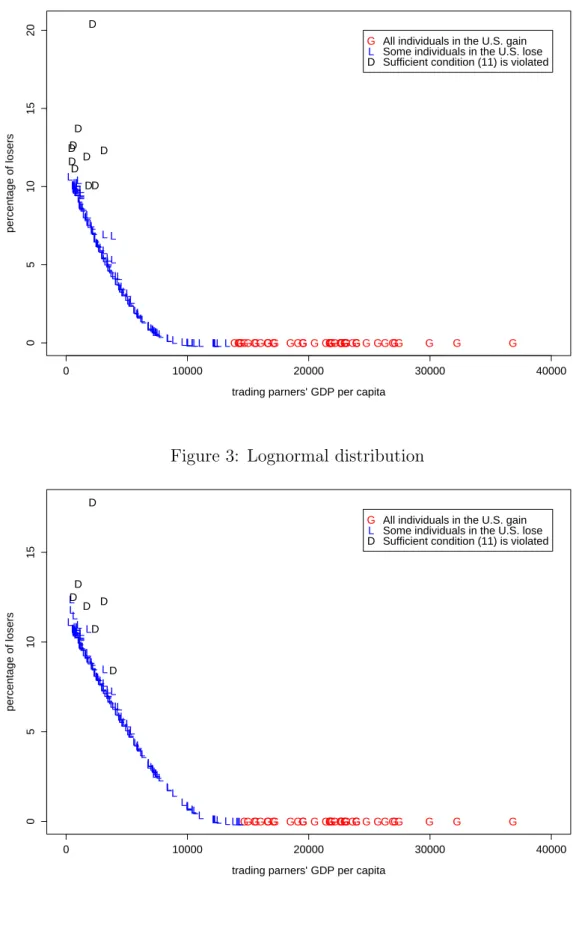
Insert Figures 2 and 3 about here.
Figures 2 and 3 depict the relationship between the share of the U.S. population who lose from trade and real GDP per capita of the trading partners for Gamma and Lognormal distributions, respectively.17 Note that U.S. intra-industry trade with countries of similar GDP
per capita makes all individuals better off because it reduces the price-wage ratios and expands the range of varieties consumed in both countries, as shown in Propositions 3 and 4. However, U.S. trade with countries having lower GDP per capita may adversely affect up to 11% of the U.S. population. The reason is that although the price-wage ratios decrease, such trade reduces product diversity in consumption. Note that when the trading partners’ GDP per capita is sufficiently small, condition (11) is violated, thus indicating that our results need to be interpreted cautiously because PPE and FPE may not hold.
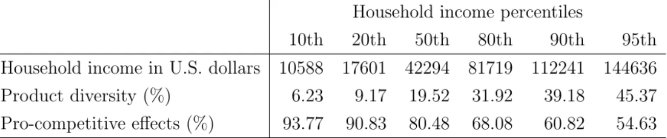
Insert Tables 1 and 2 about here.
As can be seen from Tables 1 and 2, for both income distributions, 22 out of the 28 OECD trading partners in 1997 lead to 0% of losers. For the remaining 6 OECD trading partners (Czech Republic, Greece, Hungary, Poland, Mexico, and Turkey), the percentage of losers ranges from about 0% to a maximum of almost 6% for Turkey. In other words, intra-industry trade between the OECD countries is beneficial to a broad mass of consumers. Tables 1 and 2 also show that U.S. trade with countries like China and India may yield a non-negligible share of losers in the U.S. (from about 12% to about 20%, depending on the distribution functions). In this numerical illustration, we have so far focused mainly on the share of losers in the U.S. by assuming that the U.S. actually trades with each trading partner. We can assess whether the U.S. as a whole is likely to agree on free trade with each potential trading partner. Needless to say, this requires an assumption on a relevant political process. Although such an analysis is beyond the scope of this paper, Tables 1 and 2 show that the share of potential losers is not overwhelming in all cases, thus suggesting that U.S. intra-industry trade even with highly dissimilar countries need not require protection.18
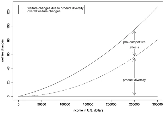
Insert Figures 4 and 5 and Table 3 about here.
Finally, we illustrate the decomposition of welfare changes at the individual level based on (22). To do this, we restrict ourselves to the Gamma distribution and focus on Canada and Mexico as U.S. trading partners. As can been seen from Table 1, there are no losers in the U.S. from trade with Canada. In the case of Mexico, however, the percentage of losers
17In what follows, we choose the following parameter values: α = 0.3; c = 0.1; and F = 0.1.
18This can be seen, for example, as follows. Recall our argument in the Introduction that compensation
mechanisms are unlikely to be operational, and consider a simple political process based on majority voting. Let bhH stand for the median of the distribution GH. Then, comparing hlossH and bhH, we see that free trade is
in the U.S. is 1.09 with the threshold hloss
H = 173687. Figures 4 and 5 illustrate how product diversity and pro-competitive effects due to trade with Canada and Mexico contribute to welfare changes for U.S. consumers depending on their income. As expected, the relative importance of product diversity increases in income in both cases. This can also be seen from Table 3, which summarizes the welfare changes due to trade with Canada for U.S. consumers at selected income percentiles.
6
Concluding remarks
Globalization is widely believed to yield gains from trade at the aggregate level, yet produces winners and losers at the individual level. In this paper, we have analyzed the impact of globalization on individual gains from trade in a general equilibrium model of monopolistic competition featuring income heterogeneity between and within countries. We have shown that, although trade always reduces markups in both countries, its impact on product diversity in consumption depends on their relative position in the world income distribution. Indeed, the range of varieties consumed in the lower income country always expands, while that in the higher income country may shrink. When the latter occurs, it is the richer consumers in the higher income country who may lose from trade because the relative importance of variety versus quantity increases with income. We have illustrated the quantitative effects of the model using data on GDP per capita and population for 186 countries, as well as parameter estimates for domestic income distributions. It turns out that U.S. trade with countries of similar GDP per capita makes all agents in both countries better off, whereas trade with countries having lower GDP per capita may adversely affect up to 11% of the U.S. population.
In order to focus entirely on how globalization affects individual welfare through product diversity and pro-competitive effects, we have developed a highly stylized model. The following two points should therefore be kept in mind when interpreting our results. First, to focus on income heterogeneity, our analysis abstracts from firm heterogeneity and trade costs (see Behrens et al., 2009, for an application of our CARA specification to firm heterogeneity and trade costs). Introducing all these elements into a single framework appears to be a promising extension in order to get a more complete picture of the impact of globalization on individual gains from trade.
Second, our analysis assumes that there is a single production factor, which rules out the role of relative factor prices in determining individual welfare. By contrast, when there is more than one factor, for instance, skilled and unskilled workers, factor proportions theory generally predicts that skilled workers in a skill abundant country will gain from trade, whereas the unskilled in that country will lose from trade. Our results thus suggest that such Stolper-Samuelson effects may get weakened or even reversed when product diversity, pro-competitive effects, and income heterogeneity are taken into account. Ultimately, trade may not generate
as much inequality in individual welfare than predicted by factor proportions theory.
Acknowledgements. We are indebted to Gianmarco Ottaviano for many useful comments on different earlier versions of this paper. We also thank Giordano Mion, Hylke Vandenbussche, and seminar participants at ARISH (Nihon University), CORE and IRES (Universit´e catholique de Louvain), RIEB (Kobe University), Konan University and KIER (Kyoto University) for helpful comments and suggestions. Kristian Behrens gratefully acknowledges financial support from the European Commission under the Marie Curie Fellowship MEIF-CT-2005-024266, from UQAM (PAFARC), and from FQRSC Qu´ebec (Grant NP-127178). Yasusada Murata gratefully acknowledges financial support from Japan Society for the Promotion of Science (17730165). This research was partially supported by the Ministry of Education, Culture, Sports, Science and Technology (MEXT, Japan), Grant-in-Aid for 21st century COE Program. Part of the paper was written while both authors were visiting KIER, while Kristian Behrens was visiting ARISH, and while Yasusada Murata was visiting CORE and UQAM. We gratefully acknowledge the hospitality of these institutions. The usual disclaimer applies.
References
[1] Arkolakis, C., S. Demidova, P. Klenow and A. Rodr´ıguez-Clare (2008) Endogenous variety and the gains from trade, American Economic Review 98, 444-450.
[2] Badinger, H. (2007) Has the EU’s Single Market Programme fostered competition? Test-ing for a decrease in mark-up ratios in EU industries, Oxford Bulletin of Economics and
Statistics 69, 497-519.
[3] Baldwin, R.E. and R. Forslid (2006) Trade liberalization with heterogeneous firms, NBER
Working Paper #12192.
[4] Balistreri, E. (1997) The performance of the Heckscher-Ohlin-Vanek model in predicting endogenous policy forces at the individual level, Canadian Journal of Economics 30, 1-17. [5] Bandourian, R., J.B. McDonald and R.S. Turley (2002) A comparison of parametric models of income distribution across countries and over time, Luxembourg Income Study Working
Papers 305.
[6] Behrens, K. and Y. Murata (2007) General equilibrium models of monopolistic competi-tion: a new approach, Journal of Economic Theory 136, 776-787.
[7] Behrens, K., G. Mion, Y. Murata and J. S¨udekum (2009) Trade, wages, and productivity,
[8] Broda, C. and J. Romalis (2009) The welfare implications of rising price dispersion. Uni-versity of Chicago, mimeographed.
[9] Broda, C. and D. Weinstein (2006) Globalization and the gains from variety, Quarterly
Journal of Economics 121, 541-585.
[10] Dixit, A.K. and J.E. Stiglitz (1977) Monopolistic competition and optimum product di-versity, American Economic Review 67, 297-308.
[11] Epifani, P. and G.A. Gancia (2009) Trade, markup heterogeneity and misallocations,
CEPR Discussion Paper #7217.
[12] Feenstra, R.C. (2004) Advanced International Trade: Theory and Evidence. Princeton, NJ: Princeton Univ. Press.
[13] Flam, H. and E. Helpman (1987) Vertical product differentiation and north-south trade,
American Economic Review 77, 810-822.
[14] Foellmi, R., C. Hepenstrick and J. Zweim¨uller (2008) Income effects in the theory of monopolistic competition and international trade, mimeographed.
[15] Gabszewicz, J.-J. and J.P. Vial (1972) Oligopoly `a la Cournot in general equilibrium
analysis, Journal of Economic Theory 4, 381-400.
[16] Hamilton, C.B. (2004) Globalization and democracy. In: Baldwin, R.E. and L.A. Winters (eds.) Challenges to Globalization: Analyzing the Economics. Chicago: The University of Chicago Press, pp.63-88.
[17] Harrison, A.E. (1994) Productivity, imperfect competition, and trade reform: theory and evidence, Journal of International Economics 36, 53-74.
[18] Helpman, E. and P.R. Krugman (1985) Market Structure and Foreign Trade. Cambridge, MA: MIT Press.
[19] Jones, R.W. (1965) The structure of simple general equilibrium models, Journal of Political
Economy 73, 557-572.
[20] Jones, R.W. (1971) A three-factor model in theory, trade, and history. In: Bhagwati, J.N., R.W. Jones, R.A. Mundell, and J. Vanek (eds.) Trade, Balance of Payments, and Growth:
Essays in Honor of Charles P. Kindleberger. Amsterdam: North-Holland, pp.3-21.
[21] Krugman, P.R. (1979) Increasing returns, monopolistic competition, and international trade, Journal of International Economics 9, 469-479.
[22] Krugman, P.R. (1980) Scale economies, product differentiation and the pattern of trade,
[23] Krugman, P.R. (1981) Intraindustry specialization and the gains from trade, Journal of
Political Economy 89, 959-973.
[24] Lawrence, C. and P.T. Spiller (1983) Product diversity, economies of scale, and interna-tional trade, Quarterly Journal of Economics 98, 63-83.
[25] Levinsohn, J. (1993) Testing the imports-as-market-discipline hypothesis, Journal of
In-ternational Economics 35, 1-22.
[26] Matsuyama, K. (2000) A Ricardian model with a continuum of goods under nonhomoth-etic preferences: demand complementarities, income distribution, and North-South trade,
Journal of Political Economy 108, 1093-1120.
[27] Mayda, A.M. and D. Rodrik (2005) Why are some people (and countries) more protec-tionist than others? European Economic Review 49, 1393-1430.
[28] Mayer, W. (1984) Endogenous tariff formation, American Economic Review 74, 970-985. [29] Melitz, M.J. (2003) The impact of trade on intra-industry reallocations and aggregate
industry productivity, Econometrica 71, 1695-1725.
[30] Melitz, M.J. and G.I.P. Ottaviano (2008) Market size, trade, and productivity, Review of
Economic Studies 75, 295-316.
[31] Neary, P.J. (2003) Globalization and market structure, Journal of the European Economic
Association 1, 245-271.
[32] OECD (2002) Intra-industry and intra-firm trade and the internationalisation of produc-tion, OECD Economic Outlook 71, 159-170.
[33] Roberts, J. and H. Sonnenschein (1977) On the foundations of monopolistic competition,
Econometrica 45, 101-113.
[34] Saint-Paul, G. (2006) Distribution and growth in an economy with limited needs: variable markups and ‘the end of work’, Economic Journal 116, 382-407.
[35] Scheve, K.F. and M.J. Slaughter (2001) What determines individual trade-policy prefer-ences? Journal of International Economics 54, 267-292.
[36] Stiglitz, J.E. (2006) Making Globalization Work. London, UK: Penguin Books Ltd.
[37] Stokey, N.L. (1991) The volume and composition of trade between rich and poor countries,
Review of Economic Studies 58, 63-80.
[38] Tybout, J.R. (2003) Plant- and firm-level evidence on “new” trade theories. In: Choi, E.K. and J. Harrigan (eds.) Handbook of International Trade. Oxford, UK: Blackwell Publishing, pp. 388-415.
Appendix A: Derivation of the demand functions
Letting λ stand for the Lagrange multiplier, the first-order conditions for an interior solution are given by:
αe−αqrr(i,hr) = λp
r(i), ∀i ∈ Ωr (23)
αe−αqsr(j,hr) = λp
s(j), ∀j ∈ Ωs (24)
and the budget constraint Z Ωr pr(k)qrr(k, hr)dk + Z Ωs ps(k)qsr(k, hr)dk = Er(hr). (25) Taking the ratio of (23) with respect to i and j, we obtain
qrr(i, hr) = qrr(j, hr) + 1 αln · pr(j) pr(i) ¸ ∀i, j ∈ Ωr.
Multiplying this expression by pr(j) and integrating with respect to j ∈ Ωr we obtain
qrr(i, hr) Z Ωr pr(j)dj = Z Ωr pr(j)qrr(j, hr)dj + 1 α Z Ωr ln · pr(j) pr(i) ¸ pr(j)dj. (26)
Analogously, taking the ratio of (23) and (24) with respect to i and j, we get:
qrr(i, hr) = qsr(j, hr) + 1 αln · ps(j) pr(i) ¸ ∀i ∈ Ωr,∀j ∈ Ωs.
Multiplying this expression by ps(j) and integrating with respect to j ∈ Ωs we obtain
qrr(i, hr) Z Ωs ps(j)dj = Z Ωs ps(j)qsr(j, hr)dj + 1 α Z Ωs ln · ps(j) pr(i) ¸ ps(j)dj. (27) Summing expressions (26) and (27), and using the budget constraint (25), we finally obtain the demands (1). The derivation of the demands (2) is analogous.
Appendix B: Proof of Proposition 1
Using (1), (2) and the definition of output per firm, it is readily verified that
QH(i)− QF(j) =− L αln · pH(i) pF(j) ¸ . (28)
Because each individual is assumed to consume all varieties, the first-order conditions (5) must hold for all firms in countries H and F . Using expression (28), one can check that
∂ΠH(i) ∂pH(i) − ∂ΠF(j) ∂pF(j) = 0 ⇐⇒ c · wH pH(i) − wF pF(j) ¸ = ln · pH(i) pF(j) ¸ . (29)
Furthermore, from expression (4) the zero profit condition requires that Πr(i) wr = · pr(i) wr − c ¸ Qr(i)− f = 0 for r = H, F.
Assume that there exists i ∈ ΩH and j ∈ ΩF such that pH(i) > pF(j). Then (29) implies that wH/pH(i) > wF/pF(j) or, equivalently, that pH(i)/wH < pF(j)/wF, whereas (28) implies that QH(i) < QF(j). Hence, ΠH(i)/wH < ΠF(j)/wF, which is incompatible with the zero profit condition at least in one country. We thus conclude that pH(i) = pF(j) must hold for all i ∈ ΩH and j ∈ ΩF, which shows that product prices are equalized. Expression (29) then shows that wH = wF, i.e., factor prices are equalized whenever product prices are equalized. Finally, setting pr(i) = ps(j) = p and wr = ws= w in (5) yields expression (9).
Appendix C: Proof of Proposition 2
We derive a sufficient condition for the symmetric price p, as given by (9), to be a price equilib-rium in the presence of income heterogeneity and finite marginal utility at zero consumption.19 To alleviate notation, we suppress subscripts whenever there is no possible confusion. Taking into account the fact that demands need not be strictly positive, aggregate demand is given by
Qr(i) = Lr R∞
0 max{0, qrr(i, hr)} dGr(hr) + Ls
R∞
0 max{0, qrs(i, hs)} dGs(hs).
We now examine under which conditions firms have no incentive to unilaterally deviate from the symmetric price (9) even when individuals are allowed not to consume all varieties. Assume that one firm charges the price ep, whereas all the other firms charge the price p given by (9). Since the deviating firm is negligible to the market, wages are unaffected and remain equalized between the two countries. The labor efficiency of the marginal consumer must satisfy qrr(ep, hl(ep)) = qsr(ep, hl(ep)) = 0, which yields (12). Letting eh ≡ hl(ep), we can rewrite the demand function of the deviating firm as follows:
Qr(ep) = Lr Z ∞ e h qrr(i, hr)dGr(hr) + Ls Z ∞ e h qrs(i, hs)dGs(hs). (30) Differentiating (30) with respect to ep and applying the Leibniz integral rule, we get:
Q0r(ep) = Lr Z ∞ eh ∂qrr(ep, hr) ∂ep dGr(hr) + Ls Z ∞ e h ∂qrs(ep, hs) ∂ep dGs(hs), (31)
where we have used the properties qrr(ep, eh) = qrs(ep, eh) = 0. The operating profit of the deviating firm is given by πr(ep) = (ep− cw)Qr(ep). Imposing symmetry on prices, on quantities, and on their derivatives, we then have
qrr(ep, hr) = whr N p − 1 αln µ ep p ¶ , ∂qrr(ep, hr) ∂ep =− 1 αep (32) qrs(ep, hs) = whs N p − 1 αln µ ep p ¶ , ∂qrs(ep, hs) ∂ep =− 1 αep· (33)
Plugging (32) and (33) into (30) and (31), we get Qr(ep) = w N p · Lr Z ∞ e h hr dGr(hr) + Ls Z ∞ e h hsdGs(hs) ¸ −1 αln µ ep p ¶ · Lr Z ∞ eh dGr(hr) + Ls Z ∞ e h dGs(hs) ¸ Q0r(ep) = − 1 αep · Lr Z ∞ e h dGr(hr) + Ls Z ∞ eh dGs(hs) ¸ .
We now classify all possible deviations from symmetry into two cases: (i) ep < p and (ii) ep > p.
Case (i): ep < p
From expression (12), we obtain eh = 0. Hence, a unilateral deviation with a lower price is not
profitable since for any ep < p we have
∂πr(ep) ∂ep = L · wh N p − 1 αln µ ep p ¶ − ep− cw αep ¸ > L · wh N p − 1 αln µ ep p ¶ − p− cw αp ¸ =−1 αln µ ep p ¶ > 0,
where we have used the definition of p in the last step.
Case (ii): ep > p
Given the result in case (i), a sufficient condition for (9) to be a symmetric price equilibrium is that ∂πr(ep)/∂ep ≤ 0 for all ep > p. This condition can be expressed as follows:
w N p · Lr Z ∞ eh hr dGr(hr) + Ls Z ∞ e h hsdGs(hs) ¸ ≤ · 1 αln µ ep p ¶ + ep− cw αep ¸ · Lr Z ∞ e h dGr(hr) + Ls Z ∞ eh dGs(hs) ¸
for all ep > p. Using (12), and because ep > p, the condition can be rewritten as
Lr Z ∞ e h hr dGr(hr) + Ls Z ∞ e h hsdGs(hs)≤ · eh + Np αw µ 1− cw ep ¶¸ · Lr Z ∞ e h dGr(hr) + Ls Z ∞ eh dGs(hs) ¸
for all ep > p. Since p/ep = e−αweh/(Np) by (12) we obtain
θReh∞hr dGr(hr) + (1− θ) R∞ e h hsdGs(hs) θReh∞dGr(hr) + (1− θ) R∞ eh dGs(hs) ≤ eh +N p αw − cN α e −αweh N p ,
where we have used the definition of the population share θ. Using p = [c + (αh/N )]w,
Appendix D: Proof of Proposition 5
The first part of Proposition 5 can be established as follows. When condition (19) holds, free trade reduces the mass of varieties consumed in country H, while the price-wage ratio decreases. Hence, two opposing effects are at work and the overall outcome is a priori ambiguous. In general, it will depend on the value of hH. To see this, we proceed as follows. First, evaluating (22) at the price equilibrium and at the equilibrium mass of firms, and differentiating the resulting expression with respect to hH, it is verified that
∂ (∆UH(hH)) ∂hH = αN αh + cNexp µ − αhH αh + cN ¶ − αnaH αhH + cnaH exp µ − αhH αhH + cnaH ¶ (34) and that ∂ (∆UH(hH)) ∂hH ¯¯ ¯ hH=0 > 0 ⇐⇒ N na H = [α + cD(L)] h [α + cD(LH)] hH > h hH , (35)
which always holds. This establishes that ∆UH is positively sloped at hH = 0. Second, note that the derivative (34) has a unique root, which is given by
hextH = (αh + cN )(αhH + cn a H) α[α(hH − h) + c(naH − N)] ln µ αhHN + cnaHN αhna H + cnaHN ¶ , (36)
such that hext
H > 0 if and only if α(hH − h) + c (naH − N) > 0. Third, since
sgn " ∂2(∆UH(hH)) ∂h2 H ¯¯ ¯¯ hH=hextH # = sgn©−£α(hH − h) + c(naH − N) ¤ª , (37)
the associated extremum is: (i) a local maximum when hext
H > 0; and (ii) a local minimum when hext
H < 0. We now analyze these two cases.
Case (i): hext
H > 0
Two sub-cases may emerge. First, when (19) holds, we have N < na
H, which then implies that limhH→∞∆UH(hH) = N − n
a
H < 0. In this case, there exists a unique threshold hlossH such that ∆UH(hH) T 0 for hH S hlossH , since (35) and ∆UH(0) = 0 hold and ∆UH is continuous in hH. Second, when (19) does not hold, we have N > naH. In this case, free trade raises the welfare of all consumers in country H through increased product diversity (N > na
H) and lower price-wage ratios (p/w < pa
H/wHa).
Case (ii): hext
H < 0
Since (35) and ∆UH(0) = 0 hold and ∆UH is continuous and strictly increasing for all hH ≥ 0, all individuals in country H gain from trade.
The second part of Proposition 5 directly result from the expansion of product diversity in consumption (N > naF) and the decrease in the price-wage ratios (p/w < paF/waF).
Figure 1: Product diversity in country H and no deviation condition when populations are homogeneous within each country
θ 1 0 1 2 hH hF (I) expand, (II) shrink, (III) shrink, (IV) expand, Φ(θ) Ψ(θ) no deviation possible deviation possible deviation no deviation
Figure 2: Gamma distribution L L L L L L GG L G G D G L G L L G L L L L L G L L L D L G L L L L D L L D L L L L L G L G L L L L L L L L L D L G G L L L G L L L L L L L L L G L G D L L L GG G L G L L L L L G G L L L L L L L G G L L L L L L G L L L L L L L L L L G G G L L D G L D L L L L L L L G G G L L L L L G L L L L G L G L L L G L L LL L L L G G L G L D L L L L L L L L L G G G L L L L D L L L 0 10000 20000 30000 40000 0 5 10 15 20
trading parners’ GDP per capita
percentage of losers
G
L
D
All individuals in the U.S. gain Some individuals in the U.S. lose Sufficient condition (11) is violated
Figure 3: Lognormal distribution
L L L L L L GG L G L D L L G L L G L L L L L G L L L L L G L L L L D L L L L L L L L G L G L L L L L L L L L D L G G L L L G L L L L L L L L L G L G D D L L GG G L G L L L L L G G L L L L L L L G G L L L L L L G L L L L L L L L L L G L G L L D G L D L L L L L L L G G G L L L L L L L L L L G L G L L L G L L LL L L L G G L G L L L L L L L L L L L G G G L L L L L L L L 0 10000 20000 30000 40000 0 5 10 15
trading parners’ GDP per capita
percentage of losers
G
L
D
All individuals in the U.S. gain Some individuals in the U.S. lose Sufficient condition (11) is violated
Figure 4: Decomposition of welfare changes due to trade with Canada (Gamma distribution) 0 50000 100000 150000 200000 250000 300000 0 20 40 60 80 100 120
income in U.S. dollars
welfare changes 0 50000 100000 150000 200000 250000 300000 0 20 40 60 80 100 120
income in U.S. dollars
welfare changes 0 50000 100000 150000 200000 250000 300000 0 20 40 60 80 100 120
income in U.S. dollars
welfare changes
welfare changes due to product diversity overall welfare changes
product diversity pro−competitive
effects
Figure 5: Decomposition of welfare changes due to trade with Mexico (Gamma distribution)
0 50000 100000 150000 200000 250000 300000 −200 −150 −100 −50 0 50
income in U.S. dollars
welfare changes 0 50000 100000 150000 200000 250000 300000 −200 −150 −100 −50 0 50
income in U.S. dollars
welfare changes 0 50000 100000 150000 200000 250000 300000 −200 −150 −100 −50 0 50
income in U.S. dollars
welfare changes
welfare changes due to product diversity overall welfare changes
product diversity
pro−competitive effects