A Micro-foundation for the Laffer Curve In a Real Effort Experiment

Texte intégral

(1)2006s-03. A Micro-foundation for the Laffer Curve In a Real Effort Experiment Louis Lévy-Garboua, David Masclet, Claude Montmarquette. Série Scientifique Scientific Series. Montréal Février 2006. © 2006 Louis Lévy-Garboua, David Masclet, Claude Montmarquette. Tous droits réservés. All rights reserved. Reproduction partielle permise avec citation du document source, incluant la notice ©. Short sections may be quoted without explicit permission, if full credit, including © notice, is given to the source..

(2) CIRANO Le CIRANO est un organisme sans but lucratif constitué en vertu de la Loi des compagnies du Québec. Le financement de son infrastructure et de ses activités de recherche provient des cotisations de ses organisations-membres, d’une subvention d’infrastructure du Ministère du Développement économique et régional et de la Recherche, de même que des subventions et mandats obtenus par ses équipes de recherche. CIRANO is a private non-profit organization incorporated under the Québec Companies Act. Its infrastructure and research activities are funded through fees paid by member organizations, an infrastructure grant from the Ministère du Développement économique et régional et de la Recherche, and grants and research mandates obtained by its research teams. Les organisations-partenaires / The Partner Organizations PARTENAIRE MAJEUR . Ministère du Développement économique, de l’Innovation et de l’Exportation PARTENAIRES . Alcan inc. . Banque du Canada . Banque Laurentienne du Canada . Banque Nationale du Canada . Banque Royale du Canada . Bell Canada . BMO Groupe financier . Bombardier . Bourse de Montréal . Caisse de dépôt et placement du Québec . Fédération des caisses Desjardins du Québec . GazMétro . Hydro-Québec . Industrie Canada . Ministère des Finances du Québec . Pratt & Whitney Canada . Raymond Chabot Grant Thornton . Ville de Montréal . École Polytechnique de Montréal . HEC Montréal . Université Concordia . Université de Montréal . Université du Québec . Université du Québec à Montréal . Université Laval . Université McGill . Université de Sherbrooke ASSOCIÉ À : . Institut de Finance Mathématique de Montréal (IFM2) . Laboratoires universitaires Bell Canada . Réseau de calcul et de modélisation mathématique [RCM2] . Réseau de centres d’excellence MITACS (Les mathématiques des technologies de l’information et des systèmes complexes) Les cahiers de la série scientifique (CS) visent à rendre accessibles des résultats de recherche effectuée au CIRANO afin de susciter échanges et commentaires. Ces cahiers sont écrits dans le style des publications scientifiques. Les idées et les opinions émises sont sous l’unique responsabilité des auteurs et ne représentent pas nécessairement les positions du CIRANO ou de ses partenaires. This paper presents research carried out at CIRANO and aims at encouraging discussion and comment. The observations and viewpoints expressed are the sole responsibility of the authors. They do not necessarily represent positions of CIRANO or its partners.. ISSN 1198-8177.

(3) A Micro-foundation for the Laffer Curve In a Real Effort Experiment Louis Lévy-Garboua*, David Masclet†, Claude Montmarquette‡ Résumé / Abstract En 1974, Arthur Laffer lançait l’idée que les recettes fiscales d’un état Léviathan se mettent à décroître lorsque le taux d’imposition excède un certain seuil. Cette idée a exercé une grande influence sur la doctrine fiscale des dernières décennies. Dans la présente étude, nous procédons à une expérience avec effort réel dans laquelle un « travailleur » est apparié à un partenaire inactif. Le but de l’expérience est de dégager les conditions de validité de la prédiction de Laffer. Nous avons retenu quatre traitements en manipulant les opportunités de travail et le pouvoir de taxer. Dans les deux traitements endogènes (avec opportunité de travail faible et forte), le participant inactif choisit le niveau de taxe qui déterminera le revenu qu’il recevra du travail de son partenaire. Dans les deux traitements exogènes, le niveau de taxe est choisi aléatoirement par l’ordinateur, et les taxes perçues distribuées au partenaire inactif. La courbe de Laffer n’est pas observable dans les traitements exogènes, mais existe bien dans les traitements endogènes, particulièrement lorsque l’opportunité du travail est forte. La recette fiscale est maximum au taux de 50 %. Nous démontrons qu’un modèle de « taxe d’efficience » (avec ou sans aversion à l’inégalité) ne parvient pas à prédire l’ensemble de ces résultats. En revanche, un modèle alternatif de préférences sociales procure des fondements microéconomiques à la courbe de Laffer. Ce nouveau modèle induit une norme sociale de juste taxation au taux de 50 % sous condition d’information asymétrique sur les types de travailleurs. Les travailleurs taxés assurent le maintien de la norme en travaillant moins lorsqu’elle n’est pas respectée, mais ne récompensent pas les choix d’imposition « généreux ». Les travailleurs qui maximisent leur richesse attendue ajustent leur travail au taux de taxation de sorte que la recette fiscale ne s’écarte pas du niveau équitable. Les travailleurs, notamment ceux qui ont une forte opportunité de travail, réagissent plus souvent de manière émotionnelle aux violations de la norme en refusant de travailler, validant ainsi la courbe de Laffer et l’histoire des révoltes de contribuables. Mots clés : asymétrie d’information, courbe de Laffer, économie expérimentale, normes sociales et sanctions, taxation et offre de travail. *. Louis Lévy-Garboua: Centre d’Economie de la Sorbonne, Université Paris I et CIRANO, 106-112, boulevard de l'Hôpital, 75013 Paris, France, Louis.Levy-Garboua@univ-paris1.fr. † David Masclet: CREM, Université Rennes I and CIRANO, 2, rue du Thabor - 35065 Rennes, et David.Masclet@univ-rennes1.fr. ‡ Claude Montmarquette, auteur pour la correspondance : Université de Montréal et CIRANO, 2020, rue University, 25e, Montréal, (Québec) Canada H3A 2A5, Claude.Montmarquette@cirano.qc.ca.

(4) A conjecture of Laffer, which had considerable influence on fiscal doctrine, is that tax revenues of a Leviathan state eventually decrease when the tax rate exceeds a threshold value. We conduct a real effort experiment, in which a “worker” is matched with a non-working partner, to elicit the conditions under which a Laffer curve can be observed. We ran four different treatments by manipulating work opportunities and the power to tax. In the endogenous treatment, the non-working partner chooses a tax rate among the set of possibilities and receives the revenue generated by her choice and the worker’s effort response to this tax rate. In the exogenous treatment, the tax rate is randomly selected by the computer and the non-working partner merely receives the revenue from taxes. The Laffer curve phenomenon cannot be observed in the exogenous treatments, but arises in endogenous treatments. Tax revenues are then maximized at a 50% tax rate. We demonstrate that an “efficiency tax” model (with or without inequity aversion) falls short of predicting our experimental Laffer curve but an alternative model of social preferences provides a microfoundation for the latter. This new model endogenously generates a social norm of fair taxation at a 50% tax rate under asymmetric information about workers’ type. Taxpayers manage to enforce this norm by working less whenever it has been violated but do not systematically reward “kind” tax setters. Workers who maximize their expected wealth adjust work to the tax rate equitably so that tax revenues remain at a fair level. Workers who respond affectively to norm violations want to hurt, and even refuse to work, so that tax revenues are cut down. Workers endowed with higher work opportunities tend to respond more emotionally to unfair taxation in our experiment, which is consistent with the observed Laffer curve and with the history of tax revolts. Keywords: experimental economics, informational asymmetry, Laffer curve, social norms and sanctions, taxation and labour supply Codes JEL : C72, C91, H30, J22.

(5) 1. Introduction The “Laffer curve” is the following proposition, attributed in 1974 to future President Reagan’s advisor Arthur Laffer by a Wall Street Journal columnist (Laffer 2004): there is a unique optimal tax rate that maximizes revenue collection. If the tax level is set below this level, raising taxes (more specifically, marginal tax rates) will increase tax revenue. However, if the tax level is set above this level, then raising taxes will decrease tax revenue. The Laffer curve is based on the commonsense intuition that tax revenues are obviously zero if the tax rate is zero, and are still zero if the tax rate is equal to one, as rational agents would withdraw from the market to evade tax or consume untaxed leisure. This conjecture of Laffer had considerable influence on fiscal doctrine, and fuelled the “supply side economics” argument that tax cut would actually increase tax revenue if the government is operating on the right side of the curve.1 Looking at the empirical literature on the effects of taxes on labor supply invites skepticism toward the Laffer conjecture (see Fortin and Lacroix (2002) for a recent survey). Indeed, many analysts conclude that net wage rates have little effect on the force participation and hours of work in employment of adult men, although women’s behavior is much more sensitive to net wages and to taxes. However, many studies have found that taxable income is much more responsive to tax changes than hours of work. In particular, high income taxpayers are always found to be very sensitive to increases in marginal tax rates because there are many ways for them to adjust to a tax increase like reducing their effort (not hours), changing the form of their compensation, switching to less taxed activities and avoiding tax. Natural experiments have become a popular method for assessing the impact of a tax policy change on taxable income (e.g. Lindsey 1987, Feldstein 1995, Goldsbee1999, Sillamaa and Veal 2000, Gruber and Saez 2002). The 1986 Tax Reform Act in the US has been under special scrutiny since the marginal tax rate on the highest-income individuals fell from 50% to 28%. One obvious limitation of natural experiments is that conclusions drawn from a specific policy change are hard to generalize to the impact of another policy and context. The use of laboratory experiments in a controlled environment circumvents this difficulty at the cost of 1. Laffer (2004) does not claim credit for this idea, which had been anticipated at least by the Islamic scholar Ibn Khaldun in the 14th century, by the French economist Frédéric Bastiat in the 19th century, and by John Meynard Keynes.. 1.

(6) limiting the study to one particular, but hopefully important, aspect of behaviour. This methodology has been used by Swenson (1988), Sillamaa (1999a, 1999b) and Sutter and Weck Hannemann (2003) to measure the effect of a wage tax on work in a real-effort experiment. We follow the same track to examine how people adjust their real work effort in response to tax rates, and we test whether a Laffer curve relates tax revenues and tax rates. Admittedly, focusing on a proportional income tax eliminates substitution possibilities between activities and assets which are partly responsible for the Laffer curve phenomenon in the highest-income groups (e.g., Feldstein 1995), and reduces the likelihood of finding a Laffer curve. The justification for this drastic simplification of reality is to demonstrate, through a controlled experiment, that the Laffer curve phenomenon does not simply arise from the conventional income - leisure trade-off. Participants are paired in the experiment. In each pair, one randomly selected participant is asked to choose and exert an effort, and the resulting output is taxed to the benefit of her partner. The working subjects in the different pairs are confronted with a set of four different tax rates (12%, 28%, 50% or 79%) and are asked to choose and perform a discrete number of real tasks conditional on the tax rate imposed on them.2 We ran four different treatments depending on work opportunities (a ceiling of 26 or 52 tasks allowed to the worker) and on the power to tax effectively given to the worker’s partner. In the endogenous treatment, the nonworking partner chooses a tax rate among the set of possibilities and receives the revenue generated by her choice and the worker’s effort response to this tax rate. In the exogenous treatment, the computer randomly selects the tax rate and the non-working partner merely receives the revenue from taxes. Thus, our experiment allows a comparison of endogenous and exogenous treatments whereas Swenson (1988) and Sillamaa (1999a, 1999b) only had an exogenous treatment and Sutter and Weck Hannemann (2003) only had an endogenous treatment. Our experiment further introduces two treatments for work opportunities. It also makes a number of technical simplifications, which make the theoretical analysis more transparent. We do not observe the Laffer curve phenomenon in our simplified setting when tax rates are randomly imposed on a working taxpayer. However, we observe it in a Leviathan state 2. The intermediate values (28%, 50%) have been chosen to coincide with the marginal tax rates on the highest income group, respectively after and before the 1986 Tax Reform Act.. 2.

(7) condition in which an experimental tax setter in flesh and blood is given the power to maximize tax revenues to his own benefit. In a bilateral bargaining game like ours, tax revenues are then maximized at a 50% tax rate beyond which they decline, notably so for treatments with high work opportunities. Benchmark predictions concerning the experiment are derived in section 2 from the conventional income–leisure trade-off (exogenous treatment) and an “efficiency tax” version of Solow’s (1979) efficiency wage model (endogenous treatment). The tax rate elasticity schedule should be unaffected by the treatment, even though a rational selfish tax setter would choose the “efficiency tax rate” that maximizes her revenue. The latter is the point on the tax rate elasticity schedule where the tax rate elasticity of tax revenue is just zero. Since no rational tax setter would fix a tax rate above this point, our benchmark is that no Laffer curve should be observed on the right side of the curve. This is clearly rejected by the data for the endogenous treatment, especially when work opportunities are high. Our experimental design is presented in more detail in section 3, and the results of our study are given in section 4. A new micro-foundation for the Laffer curve emerges in subsequent sections from a comparison between the endogenous and exogenous treatments. The fact that tax responsiveness of work is substantially greater when tax rates are set by another subject in flesh and blood than by nature is taken as evidence that workers respond strongly and emotionally to unfair taxation, which is consistent with the history of tax revolts. To be more specific, taxpayers want to punish the tax setters who intentionally violated the social norm of fair taxation. We provide an economic theory of the formation of this social norm in section 5, and of the associated punishment of norm violators in section 6, whose implications are confirmed by our experimental data. In brief, we show that a 50% tax rate is an enforceable tacit coordination rule in repeated bilateral games when workers’ types (empathy, risk aversion) are not observable by tax setters. We further demonstrate that it is cognitively rational for taxpayers to punish excessive taxation in the way predicted by equity theory (Adams 1963) in the psychological literature but it is not cognitively rational for them to reward tax gifts. We also find evidence of affective responses (Zajonc 1980) to unfair taxation by angry taxpayers who lost their temper and were ready to incur a net cost to hurt norm violators, and these turn out to be the ultimate cause for the Laffer curve phenomenon. Thus we conclude in section 7 by drawing the implications of our analysis for fiscal policy and the history of tax revolts. 3.

(8) 2. Benchmark predictions The game studied here is a two-player sequential move game that consists of two stages. The endogenous treatment reflects a situation analogous to that described by efficiency wage theory. The first player A (the “tax setter”) has the power to set the “tax rate” t∈[0,1] levied on all units of output that the second player B (the “worker”) wishes to produce in the second stage of the game. It is possible to view the tax setter, either as a non-competitive firm sharing marginal revenue with its employees, or as a Leviathan state capturing a share of earned incomes through taxes. The worker’s effort or “work” e∈[0,θ] is measured in efficiency units and equated with output. Endowed leisure time of workers is normalized to 1. The worker derives utility from her “wage” (1 − t)e and saved leisure 1 − e , and disutility from. work effort e. We define C (e) as the net disutility of work and reduction of leisure time and assume that utility is additive in wage and work W = (1 − t)e – C (e). (C ′ > 0, C ′′ > 0). (1). The tax setter picks up the revenues from the tax conditional on the worker’s effort. R = te. (2). The standard prediction of this game under the assumptions of common knowledge of rationality, selfishness and perfect information is derived by backward induction. For convenience, work and tax rates are treated as continuous variables. The worker, who is the second mover, chooses her utility (1)-maximizing effort conditional on the tax rate. For an interior optimum, the f.o.c. writes (1 − t ) − C ' (e) = 0. (3). Solving for e, the Nash equilibrium is. e* = g (t ). (4). Equation (4) describes the labour supply response to linear wage taxation, which would be observed if tax rates were exogenous.3 This condition is described by our exogenous 3. Our formulation is standard but has the undesirable feature of precluding positive tax rate elasticities of effort. Since we don’t find positive elasticities empirically and all the qualitative conclusions of our analysis extend to the more general formulation of the worker’s utility function W = V ( w + (1 − t )e, 1 − e) − C (e) , where w is the individual’s endowed wealth and V is quasi-concave, we adopted the simpler formulation for exposition.. 4.

(9) treatment. However, in the endogenous treatment, the tax setter will choose the tax rate, which maximizes her revenue (2) conditional on the worker’s effort function (4), assuming subgame perfection. The equilibrium tax rate necessarily lies strictly between 0 and 1 and is given by the f.o.c.. g (t ) + tg ' (t ) = 0. (5). This condition is analogous to the Solow condition (Solow 1979) in efficiency wage theory. The “efficiency tax rate” is such that the tax rate-elasticity of worker’s effort is just -1 or, equivalently, that the tax rate elasticity of tax revenue is just zero. This important prediction will be tested experimentally. In order to visualize which levels of taxation this condition implies, we further specify the convex cost of effort function as C (e) = δe a (δ > 0, a > 1) . The equilibrium tax rate is then 1. t* =. a −1 1 and the equilibrium effort is e* = ( 2 ) a −1 . The equilibrium tax rate is positive but a a δ. lower than one-half if1 < a < 2 , and greater than one-half if a > 2 . These benchmark predictions can be modified by introducing fairness as inequity aversion, following Fehr and Schmidt (1999) and Bolton and Ockenfels (2000). In this approach, players derive utility from the costs and returns of their actions (private component) and from the negative and positive gaps, which occur between themselves (social component). Positive returns are always good, and gaps are always bad even though disadvantageous inequity would be felt more strongly than advantageous inequity. We show in the appendix how the benchmark predictions are modified by inequity aversion when tax rates are endogenous. Efficiency tax rates will be lower than the benchmark predictions if tax setters have a weak aversion to advantageous inequity, and fall to zero (or minimum) if tax setters have a strong aversion to advantageous inequity. In addition, the tax rate elasticity of tax revenue no longer takes a negative value in the endogenous treatment but, rather, lies between 0 and 1 if tax setters have an aversion for advantageous inequity. The elasticity of tax revenue gets closer to 1 as inequity aversion rises. These results offer the way to discriminate between the two models.. 5.

(10) 3. Experimental Design At the beginning of the experiment, the participants are paired and the role played by each subject as a tax receiver (subject A) or as a taxpayer (subject B) is randomly chosen. The same roles and matching are maintained during all the experiment. Subject B, the taxpayer, produces an effort by performing a task, which consists of decoding a number from a grid of letters that appears on the computer screen. In the endogenous treatment, subject A, the tax receiver, first chooses the tax rate that she wants to impose on the number of tasks completed by B among a set of four possibilities 12, 28, 50 and 79%.4 Then, B responds to the tax rate by choosing the number of tasks that she wants to complete. Once B has decided how many tasks she wishes to perform, a first number appears, and B fills in the letter that ought to correspond to this number. Correct answers only are remunerated and taxed. The first period is completed when the last task from the number chosen by B is achieved. A is then invited to submit another tax rate to B and the game continues. This treatment evokes a context of forced taxation, in which A is the decisive member of a pressure group or a winning majority who acquired the power to tax B to her exclusive benefit. In the exogenous treatment, the tax receiver A has no power to set the tax rate, which is randomly chosen by the computer among the same set of four possibilities that was used in the endogenous treatment.5 While B is working, A is supplied with magazines and computer games to keep her waiting until the end of the session. B is aware that a randomly determined share of her own earnings will be. 4. Our endogenous treatment differs from the experimental design of Sutter and Weck-Hannemann (2003) on several details. The latter used the strategy method in which taxpayers first indicate their choice of effort for various predetermined levels of taxation and commit themselves to supply the reported effort once another player has chosen his preferred rate of taxation. They also required that the marginal income decrease with the number of tasks, which may be an unnecessary complication since the marginal disutility of effort, which cannot be controlled in a real effort experiment, is likely to increase anyway. The marginal income was kept constant in our design. Finally, Sutter and Weck-Hahnemann limited the game to only two periods and asked participants to vote on the upper limit of taxation in the second round. The effective tax rate was determined by the median vote. We are not concerned with voting in this experiment because we focus on the micro-foundations of the Laffer curve in a bilateral bargaining framework. 5 Our exogenous treatment differs from the experimental design of Swenson (1988) on several points. We keep four possibilities (12%, 28%, 50%, 79%) instead of five (12%, 28%, 50%, 73%, 87%) and measure the total effect of tax changes rather than the pure substitution effect.. 6.

(11) transferred to a passive partner and she must decide how many tasks she wants to perform.6 Not only is A’s behaviour more active in the endogenous treatment than in the exogenous treatment but this applies to B as well. In the exogenous treatment, there is no room for either non-strategic behaviour (intentions) or strategic behaviour of players, while both types of behaviour may be present in the endogenous treatment. For both the endogenous and exogenous treatments, we design two treatments, which differ by the work ceilings of subjects B, i.e. the maximum number of tasks that they are allowed to perform in each period. Work opportunities are limited to 26 tasks in the “low effort treatment”, and to 52 tasks in the “high effort treatment”. The monetary gains (leisure) of both A and B are positively (negatively) related to the number of correct tasks performed by Bs. However, taxation creates a conflict between As and Bs since it is beneficial to tax receivers and harmful to tax payers. The social marginal return for a correct task takes the constant value of 100 ECU (experimental currency units). In Table 1, we summarize the four treatments of the experiment: Table 1. Experimental treatments. Tax rate random: exogenous chosen: endogenous treatment treatment Work opportunities 26: low. Exo26 (23 pairs). Endo26 (36 pairs)7. 52: high. Exo52 (23 pairs). Endo52 (22 pairs). Each experimental session is constituted of a number of repetitions of the game. One tax rate is determined at the beginning of each game but, following Swenson (1988) and Silamma (1999a), subjects B were allowed to allocate their total work response to a game’s tax rate between three periods. This procedure is supposed to reduce errors and to avoid a restart. 6. Although As are passive in the exogenous treatment, their presence was important to maintain the same structure in both treatments and to show Bs that the tax drawn from their income was not money burning. 7 The addition of new sessions with 52 tasks led us to reduce the number of participants in those sessions relative to the initial 26 task sessions.. 7.

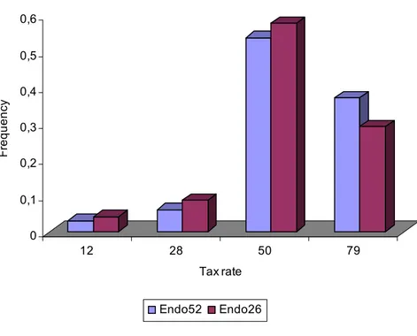
(12) effect.8 To also avoid end-game effects, subjects were not told how many repetitions of the game they would have to play. In effect, they all played six repetitions of the game over 18 periods. Since the length of each period varies according to the number of tasks chosen by B, all pairs of players did not necessarily end the experiment at the same time. This procedure allows Bs to trade-off work and leisure. The experimental sessions were run at the Lub3CE-CIRANO laboratory in Montreal. In the lab, curtains isolated participants in their respective computer booth. The experiment was computerized using the REGATE program developed by Romain Zeiliger.9 Most subjects were students. No subject had participated to previous experiments of a similar type. Once the 18 periods of play were over for a pair of players, both participants were able to leave the lab and were paid privately. On average, a session lasted 120 minutes, including initial instructions and payment of subjects, and a subject earned on average Can $ 35 including the show-up fee.. 4. Experimental results: Testing the benchmark predictions We first describe the average behavior of tax setters A (in the endogenous treatments only) and that of workers B in all treatments. Then we account for the dynamics of the behavioral response of workers to changes in tax rates, and observe whether subjects responded more strongly to intentional than to random changes. Finally, we describe tax revenues and their elasticity to tax rates, and elicit the existence conditions for a Laffer curve. 4.1. Average behaviour. Figure 1 describes the frequency with which tax setters A have chosen among the four possible tax rates in the two endogenous treatments. Very similar patterns of choice can be observed for the low effort treatment (endo 26) and the high effort treatment (endo 52). According to a Mann-Whitney test, there are no significant differences between the two treatments. A majority of subjects shared income in two halves with a non-negligible number who chose the 79% tax rate. Very few opted for tax rates lower than 50%. This result does not 8. The idea of a restart treatment has been also discussed by Andreoni (1988) in the context of voluntary contributions to public goods. 9 zeiliger@gate.cnrs.fr. 8.

(13) refute the benchmark prediction of a unique efficiency tax rate under the auxiliary assumption that there is no wide dispersion in the cost of effort function. Since tax rates rarely fall below 50%, advantageous inequity aversion, if any, should be weak for most subjects in our experiment.. Figure 1. Frequency of choice of tax rates by tax setters in the endogenous treatments 0,6 0,5. Frequency. 0,4 0,3 0,2 0,1 0 12. 28. 50. 79. Tax rate Endo52. Endo26. Figures 2a and 2b show that “workers” B always reduce their level of effort and output, measured by the number of correct tasks, when tax rates increase. This reduction of effort is strongest for the endogenous treatment and high work opportunities. A large majority of subjects perform the maximum number of tasks when tax rates are low (12%, 28%). The percentage of such high performers declines at a 50% tax rate, and even falls to zero in the endogenous treatment when tax rates peak at 79%. Average work falls from 23.3 to 18.7 tasks, when a maximum of 26 tasks can be achieved, as exogenous tax rates increase from 12% to 79%; and from 46.2 to 26.8 under the same conditions when the maximum allowance is 52 tasks. According to a Wilcoxon Sign Rank Test, in the exogenous treatments work is 9.

(14) significantly higher at the 5% significance level, both with a 12% and a 28% tax rate than with a 79% tax rate. However, work reductions appear even stronger in the endogenous treatments. In the low effort condition, average work then falls from a high of 25.2 tasks at a 12% tax rate to a low of 12.6 at a 79% tax rate. And, in the high effort condition, average work falls from a high of 49.2 at a 12% tax rate to a low of 17.3 tasks at a 79% tax rate.. Figure 2a. Average work by tax rate (range [0-26]). Average number of realized tasks. 30 25 20 15 10 5 0 12. 28. 50. 79. Tax rate endo26. exo26. 10.

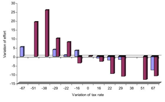
(15) Figure 2b. Average work by tax rate (range [0-52]) 50. Average number of realized tasks. 45 40 35 30 25 20 15 10 5 0 12. 28. 50. 79. tax rate endo52. exo52. 4.2. The dynamical response of workers to changes in tax rates. Figures 3a and 3b indicate the dynamical response of workers B to changes in tax rates, respectively in the low effort and the high effort treatment.. 11.

(16) Figure 3a. First differences in work with first differences in tax rates (26 tasks) 30 25. Variation of effort. 20 15 10 5 0 -5 -10 -15 -67. -51. -38. -29. -22. -16. 0. 16. 22. 29. 38. 51. 67. Variation of tax rate exogeneous treatment. endogeneous treatment. Figure 3b. First differences in work with first differences in tax rates (52 tasks) 40 30. Variation of effort. 20 10 0 -10 -20 -30 -67. -51. -38. -29. -22. -16. 0. 16. 22. 29. 38. 51. 67. Variation of tax rate exogeneous treatment. endogeneous treatment. 12.

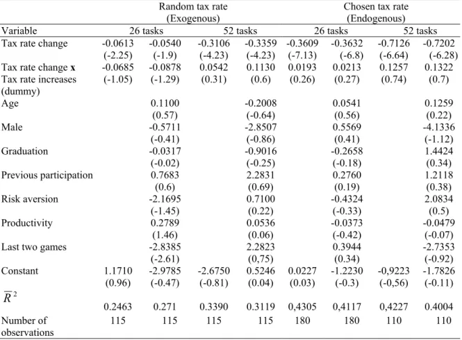
(17) These figures elicit the tax responsiveness of work by measuring how the first difference in work responds to the first difference in tax rates.10 We observe that tax changes always triggeroff work responses in the same direction. Figures 3a and 3b also allow direct comparison of tax responsiveness of work whether tax changes were intentional or not. Tax responsiveness should remain unaffected by the intentionality of tax changes according to our benchmark predictions including the modified version with inequity aversion. However, workers systematically overreacted when tax changes had been decided by a tax setter in flesh and blood. This result clearly refutes the benchmark predictions. The difference of responses for a given tax change between the two treatments is often large, and increasing in the magnitude of tax changes and of work opportunities. We can add precision to these findings by running an OLS regression of the first difference in work against the first difference in tax rates. Results for the four treatments are reported in table 2. The coefficient of tax changes in the first row measures the sensitivity of work to a tax on wages. In addition to tax changes, we added an interaction term of the latter with a dummy variable taking a value of one if tax rates have increased and zero otherwise. In the second column, we also added a number of control variables that describe the game played (two last games) and the player (average productivity in the task, age, former participation to an experiment, gender, degree and apparent risk-aversion).11 The regressions demonstrate that an increase and an equal decrease in tax rates produce symmetrical effects since the interaction term is never significant. They also confirm that tax responsiveness is strongly increasing in work opportunities, which is consistent with the fact that highest-income individuals are particularly sensitive to tax changes. Furthermore, tax responsiveness seems to be exacerbated by the possibility to identify the tax receiver with a person in flesh and blood who intentionally set the rate of transfer to his exclusive benefit. We believe that this is a new and important finding that requires explanation. Finally, looking at the second column, we observe that, with a single exception, control variables are never significantly different from zero at the 5% level. 10. We take the average work during the three periods of one game. The “two last games” variable is a dummy taking value one in the two last games and zero otherwise. It might capture uncontrolled end-game behavior of players and fatigue. The player’s productivity in the experimental task is obtained by dividing the total number of correct tasks by the time spent on these tasks. It captures the player’s task-specific ability. Besides, subjects were classified as “risk-averse” if they preferred a $5 show-up fee to a lottery ticket that gave them a 50% chance to get $11 and nothing otherwise. The lottery was drawn at the end of the session.. 11. 13.

(18) We interpret this result as evidence that (prior) tax changes have a causal effect (in Granger’s sense) on work changes. Table 2. OLS regressions of first differences in work by treatment. Variable Tax rate change Tax rate change x Tax rate increases (dummy) Age. Random tax rate Chosen tax rate (Exogenous) (Endogenous) 26 tasks 52 tasks 26 tasks 52 tasks -0.0613 -0.0540 -0.3106 -0.3359 -0.3609 -0.3632 -0.7126 -0.7202 (-2.25) (-1.9) (-4.23) (-4.23) (-7.13) (-6.8) (-6.64) (-6.28) -0.0685 -0.0878 0.0542 0.1130 0.0193 0.0213 0.1257 0.1322 (-1.05) (-1.29) (0.31) (0.6) (0.26) (0.27) (0.74) (0.7). Male Graduation Previous participation Risk aversion Productivity Last two games Constant. R2. 1.1710 (0.96). 0.2463 Number of 115 observations Note: t values are in parentheses.. 0.1100 (0.57) -0.5711 (-0.41) -0.0317 (-0.02) 0.7683 (0.6) -2.1695 (-1.45) 0.2789 (1.46) -2.8385 (-2.61) -2.9785 (-0.47) 0.271 115. -2.6750 (-0.81). -0.2008 (-0.64) -2.8507 (-0.86) -0.9016 (-0.25) 2.2831 (0.69) 0.7100 (0.22) 0.0536 (0.06) 2.2823 (0,75) 0.5246 (0.04). 0.3390 115. 0.3119 115. 0.0227 (0.03). 0.0541 (0.56) 0.5569 (0.41) -0.2658 (-0.18) 0.2760 (0.19) -0.4324 (-0.33) -0.0373 (-0.42) 0.3944 (0.34) -1.2230 (-0.3). -0,9223 (-0,56). 0.1259 (0.22) -4.1336 (-1.12) 1.4424 (0.34) 1.2118 (0.38) 2.0834 (0.5) -0.0479 (-0.07) -2.7353 (-0.92) -1.7826 (-0.11). 0,4305 180. 0,4117 180. 0,4227 110. 0.4004 110. 4.3. Tax revenue and the Laffer curve. Figure 4 shows the variation of tax revenue with tax rates in the endogenous treatments. The tax revenue increases up to the 50% tax rate and decreases thereafter, most visibly so in the high effort treatment. Thus, we obtain a Laffer curve and confirm the experimental findings of Sutter and Weck Hannemann (2003) in this respect. However, if we move to the exogenous treatments, the tax revenue increases steadily with tax rates in the observed range (not shown). No Laffer curve can be found then within reasonable bounds for tax rates. 14.

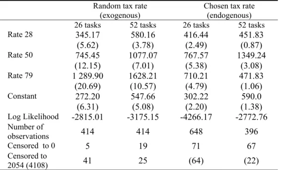
(19) Figure 4. Tax revenue by tax rates for the endogenous treatments 2000 1800 1600. Tax revenue. 1400 1200 1000 800 600 400 200 0 12. 28. 50. 79. Tax rate endo26. endo52. In order to characterize the Laffer curve more precisely, we run a Tobit regression on tax revenues as a function of tax rate dummies for the 4 treatments. The results reported in Table 3 obviously do not support the existence of a Laffer curve whenever tax rates are exogenous. The latter appears only in a weak (or degenerate) sense for endogenous rates in the low effort treatment (26 tasks) insofar tax revenue reaches a maximum at a 50% tax rate but remains approximately constant thereafter. Finally, the Laffer curve emerges strikingly in the endogenous high effort treatment (52 tasks) since tax revenue reaches a high peak at the 50% tax rate and falls to non-significant values both at lower and higher tax rates.. 15.

(20) Table 3. Determinants of tax revenue Random tax rate (exogenous) 26 tasks 52 tasks Rate 28 Rate 50 Rate 79 Constant Log Likelihood Number of observations Censored to 0 Censored to 2054 (4108). Chosen tax rate (endogenous) 26 tasks 52 tasks. 345.17 (5.62) 745.45 (12.15) 1 289.90 (20.69) 272.20 (6.31) -2815.01. 580.16 (3.78) 1077.07 (7.01) 1628.21 (10.57) 547.66 (5.08) -3175.15. 416.44 (2.49) 767.57 (5.38) 710.21 (4.79) 302.22 (2.20) -4266.17. 451.83 (0.87) 1349.24 (3.08) 471.83 (1.06) 590.0 (1.38) -2772.76. 414. 414. 648. 396. 5. 19. 71. 67. 41. 25. (64). (22). Note: t values are in parentheses. Table 4. Elasticity of tax revenue to tax rates. η12 η12,28 = η20 η28 η28,50 = η39 η50 η50,79 = η64,5 η79. Random tax rate (exogenous) 26 tasks 52 tasks. Chosen tax rate (endogenous) 26 tasks 52 tasks. 0.702 0.739. 0.574 0.565. 0.654 0.629. 0.181 0.363. 0.775 0.825. 0.556 0.543. 0.604 0.569. 0.545 0.795. 0.857 0.898. 0.567 0.598. 0.279 -0.104. 0.033 -0.973. 0.939. 0.629. -0.487. -1.978. The unconditional expectations are predicted from the regressions on tax revenues given in Table 3. Elasticities are computed from estimates of EQ1 and EQ2 at two adjacent tax rates (e.g., 12 and 28%), at the three mean points (20, 39 and 64.5%), by the formula: ( EQ2 − EQ1 ) / ( EQ2 + EQ1 ) / 2 . The three mid-point elasticities were then extrapolated linearly (T2 −T1 ) / (T2 +T1 ) / 2 to the four tax rates.. 16.

(21) Coefficients exhibited in table 4 are then converted into elasticity values of tax revenue for various tax rates. The computed elasticity values reported in table 4 are always positive and fairly constant if tax rates are set randomly. They are consistent with the taxable income elasticity of 0.4 that Carroll and Hrung (2005) view as typical for higher-income taxpayers in the recent literature. The picture is totally different if tax rates are set intentionally. Then, the elasticity of tax revenue is positive at lower-than-fifty percent tax rates and turns suddenly null or negative above this threshold. A strongly negative elasticity obtains in the high effort treatment. To sum up, the Laffer curve is strongly suggested on our experimental data by a comparison between the endogenous and exogenous treatments. Clearly, the tax rate elasticity of tax revenue lies between 0 and 1 (even between 0.5 and 1 on our dataset) when a computer randomly selects tax rates, but falls significantly to 0 and below in both low effort and high effort treatments when tax rates are chosen by another subject in flesh and blood. The efficiency tax model does not accomplish a bad job since it manages to predict that tax rates should be heavily concentrated at their efficiency value and the tax rate elasticity of tax revenue should just equal 0 in the endogenous treatments. However, it cannot predict that the observed efficiency tax rate be close or equal to one-half, or that the tax rate elasticity of tax revenue may become strictly negative. By extrapolation of the estimated values, the tax rate elasticity of tax revenue computed from the exogenous treatments would suggest an efficiency tax rate derived from the benchmark model well above 79% and probably close to one, therefore much too high to fit the data. Results from the endogenous treatments refute even more the inequity aversion modification of this model since the latter predicts smaller efficiency tax rates than the benchmark predictions, and a tax rate elasticity of tax revenue between 0 and 1 if tax setters have an aversion to advantageous inequity. In the next section, we develop a new dynamic micro-foundation for the Laffer curve that can predict all of our experimental results. The fact that the tax rate elasticity of tax revenue is substantially negatively lower when tax rates are set by another subject in flesh and blood than. 17.

(22) by nature is taken as evidence that taxpayers want to punish the tax setters who intentionally violated the social norm of fair taxation.12. 5. The social norm of fair taxation: 5a. Determining prior intentions and normative expectations of players:. Since we cannot rely solely on the benchmark efficiency tax model or on a social preference model with inequity aversion to make sense of our experimental data, we may turn to an intention-based reciprocity model (Rabin 1993, Dufwenberg and Kirchsteiger 2004). However, these models have serious deficiencies in their present state because they don’t answer the basic question: “How can B read A’s intentions?” We answer this question here by using an approach developed by Lévy-Garboua, Meidinger and Rapoport (2004: sections 5-6), which reformulates the psychological mechanisms of social cognition in the terms of social choice theory. Prior intentions of rational players in the endogenous treatments are assimilated to their normative expectations before the game starts, conditional on the rules of the game. Since the latter appear to be common to all players or to a specific group of players in our experimental setting, they are common knowledge and may constitute a group norm or a social norm. Forward-looking subjects anticipate that they will be playing either role (A or B) during the whole session (partner treatment) with an equal probability. Although they make a choice for several successive games, rational players must plan a constant behaviour over all future games before the game starts, since they possess exactly the same information on all future periods. Therefore, we may assume a single game to determine the prior social preference. Let us further assume for the time being that the subject believes that her unknown partner is similar to self (in-group condition). Although she will control either taxation or work in reality but not both, she can imagine, before the game starts, that her similar partner would make the same choice than herself of the behavior that she controls. Thus she maximizes her statedependent expected utility by imagining herself either in the A state or in the B state and by 12. If taxpayers were unable to conceive forward-looking strategies, they would quickly learn their partner’s type (fair or selfish) and comply with it, since the same pairs of partners are matched for an indefinite number of games in our endogenous treatments. Given this fact, even fair tax setters would be tempted to take advantage of their partner’s myopia under asymmetric information about types and reveal a selfish type. Obviously, they don’t.. 18.

(23) projecting her own characteristics (initial wealth, VNM utility function, cost of effort) onto her unknown, but similar, partner 1 1 max EU (t , e) = U ( w + te) + [U ( w + (1 − t )e) − C (e)] t ,e 2 2 s.t. 0 ≤ t ≤ 1, 0 ≤ e ≤ θ. , (U ′ > 0, U ′′ < 0). (11). Lemma 1:. In the in-group condition, a 50% tax rate is a group norm for risk-averse partners. This norm is invariant to work opportunities θ. Proof: We calculate the two first-order derivatives of (11). ∂EU 1 = e[U ′( w + te) − U ′( w + (1 − t )e)] ∂t 2 ∂EU 1 = [tU ′( w + te) + (1 − t )U ′( w + (1 − t )e) − C ′(e)] ∂e 2 We first rule out the zero effort condition since all subjects have agreed to participate to the experiment. From now on, e ≠ 0 is assumed everywhere for work intentions. Hence, the taxation optimum under perceived homogeneity of participants is easily derived from the first expression under concavity of the VNM utility function: t* =. 1 .□ 2. The optimal tax rate under perceived homogeneity of players or empathy13 can serve as a group norm for risk-averse players because it is independent from individual characteristics (initial wealth, risk aversion, cost of effort). Therefore, rational players are aware of prior intentions of their partners and can tacitly coordinate their own decisions. Furthermore, this norm does not vary with work opportunities. It is worth noticing that the group norm prescribes equalization of earnings, not of utility. Only marginal utilities of wealth are equalized, and the worker gets no compensation for his work. This result is a well-known consequence of state-dependent EU (Cook and Graham 1977). Players prefer to be tax setters than workers and take no coverage against the risk of becoming workers when they are unable to exchange this loss on markets.. 13. In many psychological studies, empathy is manipulated by making subjects perceive their similarity (high empathy) or dissimilarity (low empathy) with others.. 19.

(24) Let us now assume more generally that players have limited empathy or perceive heterogeneity in the sense that they will be confronted to a “similar” partner (in-group condition) with probability λ ( 0 ≤ λ ≤ 1) or to a “dissimilar” partner (out-group condition) with probability 1-λ. Moreover, they have an equal chance of playing either A or B. Letting, in the out-group condition, t designate the tax rate set exogenously by the partner and e the exogenous effort of the partner, we write the state-dependent EU: 1 1  EU (t , e, t , e , λ ) = λ  U ( w + te) + (U ( w + (1 − t )e) − C (e) ) 2 2  1 1  + (1 − λ )  U ( w + te ) + (U ( w + (1 − t )e) − C (e) ) 2 2 . (12). Prior intentions are now derived by maximizing (12) with respect to e and t under quantity constraints. Prior tax rates exhibit a general pattern described by the following proposition. Lemma 2:. Before the game starts, no risk-averse player expects the tax rate to be smaller than one-half even though she perceives heterogeneity. Proof: Once again, e, e ≠ 0 are assumed. The first derivative of (12) with respect to t yields:. ∂EU 1 1 = λ e[U ′( w + te) − U ′( w + (1 − t )e)] + (1 − λ ) e U ′( w + te ) . ∂t 2 2 ∂EU (t = 1 2, λ < 1) 1 From the latter, we derive: = (1 − λ ) e U ′( w + te ) > 0 , which demonstrates that ∂t 2 the taxation optimum under perceived heterogeneity is greater than one-half. After allowing for discrete choice of tax rates and the special case of perceived homogeneity (λ = 1) , we get the general proposition. □. Since tax rates are discrete in our experiment and only take two values no smaller than onehalf, the optimal tax rate is one-half for small-perceived heterogeneity and equal to 0.79 for great-perceived heterogeneity or selfishness. It is also likely to increase with work. 20.

(25) opportunities if partial risk aversion is smaller than one, as usually postulated.14 The optimal tax rate is no longer a common prior as it now depends on individual characteristics of players. However, it still defines the “normative expectation” of future workers. 5b. Social norm of fair taxation and the micro-Laffer curve:. If workers have a prior social preference on entering the game, they must have a normative expectation for the tax rate. Since the tax rate that was chosen by A can be different from B’s normative expectation, B will experience surprises. Observing a tax rate in excess of one’s norm is an unpleasant surprise, which causes a feeling of outcome dissatisfaction, and observing a tax rate below the norm is a pleasant surprise, which causes satisfaction (LévyGarboua and Montmarquette 2004). Bad and good surprises generate a potential for dynamic strategies of players, like the punishment of norm violators by unsatisfied workers and the reward of kind tax setters by satisfied workers. How effective will these dynamic strategies be? This is the point that we now have to examine. The main assumption that we make in the sequel of the paper is the following. Assumption A:. The tax rate elasticity of tax revenue is positive when tax rates are exogenous and do not exceed 50%. This assumption is consistent with our observation (table 5) that the measured elasticity of tax revenue in the exogenous treatment is 0.857 (0.939) in the low effort treatment and 0.567 (0.629) in the high effort treatment for a 50% (79%) tax rate. Consequently, tax setters have an incentive to set the tax rate above one-half since this would increase their revenue. In our experiment, they would have an incentive to opt for a 79% tax rate. Such tax rate would fit the normative expectation of the most selfish workers and cause dissatisfaction to others. However, even selfish (or risk-loving) workers would stand to gain from lower taxation. If it is common knowledge that no risk-averse player expects tax rates to be lower than one-half. 14. If. partner’s. work, e ,. increases. with. work. opportunities,. ∂ 2 EU (t = 1 2, λ < 1) 1 = (1 − λ ) 2 ∂t∂e.  e U ′′( w + te )  U ′( w + te ) 1 +  >0. The term in brackets is equal to one minus the partial risk aversion  2 U ′( w + te )  coefficient calculated for the tax revenues expected from a dissimilar worker who is charged a 50% tax rate.. 21.

(26) (lemma 2), those workers whose normative expectation exceeds one-half would benefit from exploiting the informational asymmetry on type (empathy, risk aversion) and pretend that they, too, expected a 50% tax rate. Consequently, all workers would want to enforce the social norm of a 50% tax rate, whether the latter does truly reflect their idiosyncratic normative expectation or not. Proposition 1:. If lemma 2 is common knowledge and types (empathy, risk aversion) are not observable by tax setters, a 50% tax rate is recognized as a social norm that rational workers of all types wish to enforce on tax setters. A direct confirmation of lemma 2 and proposition 1 is provided by a comparison of choice of tax rates by tax setters in the first game and subsequent games. Under perceived heterogeneity, we showed (lemma 2) that the optimal tax rate is one-half for small-perceived heterogeneity and equal to 0.79 for great-perceived heterogeneity or selfishness. We expect this situation to reflect choices of tax setters in the first game, that is, before they could experience the worker’s response to their own move. Furthermore, we showed that the optimal tax rate is likely to increase with work opportunities if partial risk aversion is smaller than one, as usually postulated. That is, the first choice should be more biased toward the 79% rate in the high effort treatment than in the low effort treatment. This is exactly what can be seen on figure 5. Thus, we have reasons to suspect that subjects have limited empathy or perceive heterogeneity. However, if types are unobservable, proposition 1 states that workers should wish to enforce the 50% social norm on tax setters by punishing norm violators. Indeed, the comparison between figure 1 and figure 5 demonstrates that most tax setters comply with the social norm of equal sharing of income in subsequent games.. 22.

(27) Figure 5. Frequency of choice of tax rates by tax setters in the first game in endogenous treatments. 0,8 0,7. Frequency. 0,6 0,5 0,4 0,3 0,2 0,1 0 12. 28. 50. 79. Tax rate for first game Endo52. Endo26. 6. Punishment of norm violators: Fully rational workers will have the power to enforce a 50% tax rate if two conditions are met: (i) tax setters fail to earn additional revenues by being punished whenever they increase tax rates above one-half; (ii) workers do not lose from punishing norm violations. In our experimental setting, punishment of norm violators remains implicit. Since a 50% tax rate is recognized as a social norm, it is common knowledge that observed punishments in one game would be repeated under the same conditions in all future games. Therefore, a tax setter who currently loses revenues after being punished once for violating the 50% norm is sure to lose if he keeps on violating the norm in the future. Let t > 1 2 be the tax rate chosen by the tax setter, g (t ) the worker’s best work response to this tax rate (see eq. (4)) and W n (t ) = (1 − t ) g (t ) − C ( g (t )) designate her Nash utility. B punishes A for imposing a tax rate that was above the social norm by choosing to work e(t ) < g (t ) such 23.

(28) that A gets revenues which are lower than expected in the current game and no higher than the revenues he would have got by respecting the social norm: te(t ) ≤ 1 2 g (1 2) ≡ R n (1 2). (13). The worker obtains currently a lower utility by punishing (W p (t ) = (1 − t )e(t ) − C (e(t ))) than by playing Nash (W n (t ) > W p (t )) . However, any punishment consistent with (13) forces the tax setter to respect the norm in the T remaining games in order to escape repeated losses. The worker expects from A’s compliance with the social norm a permanent utility level W n (1 2) which is higher than her Nash utility. “Equitable punishment” is chosen so as to maximize worker’s current utility W p (t ) under constraint (13). The punished A receives a revenue which is lower than what he expected to get by violating the norm, and no higher than what he would have obtained by complying with the social norm. Equitable punishment is effective only if B does not lose from punishing the norm’s violation: W p (t ) + TW n (1 2) ≥ (1 + T )W n (t ) ,. [. ]. or. T W n (1 2) − W n (t ) ≥ W n (t ) − W p (t ) .. (14). This last condition states that equitable punishment is a profitable private investment with a non-negative return. Punishment is made effective, and the social norm is respected, when the game is infinitely repeated but it is eventually violated when the number of repetitions is too small. As an alternative to equitable punishment, which is a cognitive, cold and fully rational response to norm violation and a mere compensation for damage, “revenge” is an affective, hot and bounded rational drive, which aims at hurting norm violators. Under a strong feeling of unfair treatment, the cognitive process is inhibited and workers stay hooked on their prior normative preference for a fair tax. They express anger and unconditionally deny tax setters the right to be unfair. Hurting norm violators is the way to burn the latter’s illegitimate profits. Emotional (impulsive) responses of this kind are usually observed in cases of emergency and they often take the form of all-or-nothing response (Zajonc 1980). Their existence is attested by the fact that responders commonly reject unfair proposals and accept fair proposals in oneshot ultimatum games. Revenge is prevalent in one-shot games but may also be present in 24.

(29) finitely repeated games. Presumably, a fraction of workers will have an emotional response to norm violations and this fraction should increase with the distance to the social norm. Proposition 2:. If taxpayers punish equitably tax setters who violated the social norm of 50% tax rate, a Laffer curve can be observed in a weak form, i.e. the tax rate elasticity of tax revenue falls permanently to zero beyond the 50% threshold. If some workers punish norm violators out of revenge and other workers punish norm violators equitably, a Laffer curve can be observed in a strong form, i.e. the average tax rate elasticity of tax revenue becomes permanently negative beyond the 50% threshold. The maximum tax revenue is obtained for a 50% tax rate. Proof: If t > 1 2 , equitable workers punish tax setters by choosing work so as to maximize. W p (t ) = (1 − t )e − C (e) s.t. 0 ≤ e ≤. R n (1 2) ≡ emax (t ) . t. Since. emax (t ) < g (t ) and C ′′ > 0 ,. C ′(emax (t )) < C ′( g (t )) = 1 − t . Hence, equitable workers punish norm violators by choosing emax (t ) . Since temax (t ) ≡ R n (1 2) , the violator always gets the same tax revenue than by respecting the social norm of 50% tax rate and the tax rate elasticity of revenue is just equal to zero. If some workers respond emotionally to norm violations by ceasing to work, tax revenues decrease in the aggregate and the tax rate elasticity of revenue becomes negative. □. It is worth noticing that our description of “equitable punishment” exactly confirms Adams’ (1963) “equity theory” (see also Akerlof and Yellen 1990). This result nicely relates fair taxes (wages) to a dynamic version of efficiency taxes (wages). So far, we haven’t ruled out the possibility that the optimal tax rate be lower than 50%. This would happen if it pays a rational tax setter to be “kind” toward workers by setting the tax rate below the 50% norm. This is not the case, however. Proposition 3:. Under assumption A, it is not equitable for a tax setter to be kind toward the worker by setting the tax rate below the 50% norm. Proof: Assume that t < 1 2 and that worker B “rewards” the kind tax setter A by working more than it is optimal and enough to ensure that A gets no less revenue than R n (1 2) .. e(t ) ≥. That is,. n. R (1 2) ≡ emin (t ) . t 25.

(30) (i) By the assumption that that exogenous tax rate elasticity of revenue is positive, tg (t ) < R n (1 2) for. all t < 1 2 . Hence, emin (t ) > g (t ) . (ii) If emin (t ) > g (t ) , worker B chooses the minimum effort level emin (t ) that will reward the kind tax setter and reaches a suboptimal utility level while A gets the same tax revenue than he would obtain by respecting the social norm of 50% tax rate. Thus, B has no incentive to reward A’s kindness, and, knowing this, A has no incentive to be kind either. □. Although there will be no equitable reward to a kind tax setter who chose a tax rate which is below the 50% norm, some workers may feel gratitude toward their kind partner and wish to reward her at their own expense. Strong positive emotions are susceptible to trigger-off rewards in one-shot or finitely repeated games. However, it is likely that that the absence of equitable reward will dominate in the aggregate and cause the average tax rate elasticity of revenue to be positive. Thus, tax revenue is likely to increase with tax rate until it reaches the 50% social norm and stops increasing, or even decrease, at higher rates. The asymmetry of equitable rewards and punishments is responsible for a dynamic inversely U shaped Laffer curve. Proposition 4:. Under assumption A, an aggregate Laffer curve is likely to exist and the maximum tax revenue is obtained at a 50% tax rate. We have ample evidence of punishment/reward strategies from our experimental setting. In figures 2a and 2b, we found that workers responded more strongly to endogenous tax changes than to exogenous ones. The observed gap between the mean responses in the two treatments indicates the amount of punishment and reward. Since equitable rewards have been ruled out (proposition 3), the observed rewards following a tax reduction must be driven by affect and thus appear to be large on figs. 2a and 2b. However, they are barely observed (tables 1 and 5). By contrast, a majority of punishments following norm’s violations are driven by equity and this limits the average magnitude of observed punishments. However, affective punishments should be more frequent if workers face high work opportunities. Since affect-driven punishments often take the form of all-or-nothing responses, we should observe that workers refuse to work more frequently after a norm’s violation in the high effort treatment than in the low effort treatment. Indeed, we can calculate from the bottom of table 4 that 16.9% refuse to work with a maximum of 52 tasks vs. 11.0% with a maximum of 26 tasks. 26.

(31) 7. Conclusion: Implications for fiscal policy and the history of tax revolts Our experiments show that a Laffer curve phenomenon cannot be observed when tax rates are randomly imposed on a working taxpayer, but arises in a Leviathan state condition in which a tax setter is given the power to maximize tax revenues to his own benefit (Brennan and Buchanan 1979, Buchanan 1979). Tax revenues are then maximized at a 50% tax rate. These results confirm Laffer’s conjecture that a Laffer curve would exist at a reasonable threshold, even if taxpayers had only one source of income. However, the reasons why a Laffer curve exists defy conventional economic wisdom but conform to basic political instinct. Our experimental findings suggest that, most of the time, fiscal changes will not produce a Laffer effect. Fiscal policies that serve macroeconomic purposes are likely to be perceived as exogenous changes by taxpayers. In order to produce a Laffer effect, fiscal policies need to be felt as intentional, discriminatory and especially hurtful by a group of taxpayers. The latter feel inequitably treated under such conditions, and those who feel it most strongly lose their temper and react emotionally to the breach of the implicit social norm. To be more specific, the workers who respond more emotionally to unfair taxation tend to be those endowed with higher work opportunities, and this is consistent with the history of tax revolts. The initiators of tax revolts are usually found among the most productive, high earning, and hard-working group of taxpayers. For instance, the quest for American independence grew as issues like taxation without representation in the British government angered the local population of the former British colonies. When the British decided to tax the colonists to pay a share of their expensive war against the French and Indians, the colonists were angry and rallied behind the phrase, “No Taxation without Representation”. The British were then forced to remove (1764-1767) most of the unfair taxes (tax on sugar, Stamp Act, Townsend Act) that they had been trying to enforce unilaterally. Two centuries later, the same scenario repeated in California as property taxes went out of control. Taxpayers were losing their home because they could not pay their property taxes, yet government maintained the burden. In the tradition of the American colonists, California taxpayers stood up and passed Proposition 13 (1978) that reduced property taxes by about 57%. The tax revolt that swept the country had a worldwide impact. 27.

(32) Our experiments demonstrate in a highly stylized fashion that the Laffer effect characterizes tax revolts, that is, an affective rejection of discriminatory and hurtful taxation. The Laffer curve phenomenon considerably exceeds the predictable outcome of a standard income-leisure trade-off; and it even exceeds the magnitude of cognitively rational reactions to inequity. An important goal of our paper was to provide a rigorous micro-foundation for the Laffer curve. This new model uses simple tools of social choice theory to formulate prior intentions of players and endogenously generate a social norm of fair taxation at a 50% tax rate under asymmetric information about workers’ type. Taxpayers manage to enforce this norm by working less whenever it has been violated but do not systematically reward kind tax setters. Workers who maximize their expected wealth adjust work to the tax rate equitably so that tax revenues remain at a fair level. Remarkably, these workers conform to equity theory (Adams 1963), but only for disadvantageous inequity. Workers who respond affectively to norm violations want to hurt and even refuse to work so that tax revenues are cut down. The Laffer curve arises both from the asymmetry of equitable rewards and punishments and from the presence of a substantial share of emotional rejections of unfair taxation.. 28.

(33) References Adams, J. (1963), “Toward an Understanding of Inequity”, Journal of Abnormal and Social Psychology 67, 422-436. Akerlof, G.A. and J.L. Yellen (1990), “The Fair Wage- Effort Hypothesis and Unemployment”, Quarterly Journal of Economics 105:255-284. Andreoni, J. (1988), “Why Free Ride? Strategies and Learning in Public Goods Experiments”, Journal of Public Economics 37, 291-304. Bolton, G. and A. Ockenfels (2000), “A Theory of Equity, Reciprocity and Competition”, American Economic Review 100, 166-193. Brennan, G. and J. M. Buchanan (1979), “The Logic of Tax Limits: Alternative Constitutional Constraints on the Power to Tax”, National Tax Journal 32, 11-22. Buchanan, J. M. (1979), “The Potential for Taxpayer Revolt in American Democracy”, Social Science Quarterly 59, 691-696. Carroll, R. and W. Hrung (2005), “What Does the Taxable Income Elasticity Say About Dynamic Responses to Tax Changes?”, American Economic Review 95, 426-431. Dufwenberg, M. and G. Kirchsteiger (2004), “A Theory of Sequential Reciprocity”, Games and Economic Behavior 47, 268–298. Fehr, E. and K. Schmidt (1999), “A Theory of Fairness, Competition and Cooperation“, Quarterly Journal of Economics 114, 817-868. Feldstein, M. (1995), “The Effect of Marginal Tax Rates on Taxable Income: A Panel Study of the 1986 Tax Reform Act”, Journal of Political Economy 103, 551-572. Fortin, B. and G. Lacroix (2002), “Assessing the Impact of Tax and Transfer Policies on Labour Supply: A Survey”, CIRANO project report, 43p. Goldsbee, A. (1999), “Evidence on the High-Income Laffer Curve from Six Decades of Tax Reform”, Brookings Papers on Economic Activity, 1-47. Gruber, J. and E. Saez (2002), “The Elasticity of Taxable Income: Evidence and Implications”, Journal of Public Economics 84, 1-32. Laffer, A. (1974), “The Laffer Curve: Past, Present, and Future”, Heritage Foundation Backgrounder #1765. Lévy-Garboua L., Meidinger, C. and B. Rapoport, (2004), “The Formation of Social Preferences: Some Lessons from Psychology and Sociology”, in: S.C. Kolm, J. MercierYthier, eds. Handbook of the Economics of Giving, Altruism and Reciprocity, Amsterdam: Elsevier, forthcoming. Lévy-Garboua, L. and C. Montmarquette (2004), “Reported Job Satisfaction: What Does it Mean?”, Journal of Socio-Economics 33, 135-151. 29.

(34) Lindsey, L.B. (1987), “Individual Taxpayer Response to Tax Cuts: 1982-1984: With Implications for the Revenue-Maximizing Tax Rates”, Journal of Public Economics 33, 173206. Rabin, M.(1993), “Incorporating Fairness into Game Theory and Economics”, American Economic Review, 83, 1281-1302. Sillamaa, M.A (1999a), “Taxpayer Behavior in Response to Taxation: Comment and New Experimental Evidence”, Journal of Accounting and Public Policy 18, 165-177. Sillamaa, M.A (1999b), “How Work Effort Responds to Wage Taxation: an Experimental Test of a Zero Top Marginal Tax Rate”, Journal of Public Economics 73, 125-134. Sillamaa, M.A. and M. Veal (2000), “The Effects of Marginal Tax Rates on Taxable Income: A Panel Study of the 1988 Tax Flattening in Canada”, Research Report no 354. Solow, R. (1979), “Another Possible Source of Wage Stickiness”, Journal of Macroeconomics 1, 79-82. Sutter, M. and H. Weck-Hannemann, (2003), “Taxation and the Veil of Ignorance: A Real Effort Experiment on the Laffer Curve”, Public Choice 115, 217-240. Swenson, C. (1988), “Taxpayer Behavior in Response to Taxation: an Experimental Analysis”, Journal of Accounting and Public Policy 7, 1-28. Zajonc, R.B. (1980), “Feeling and Thinking: Preferences Need No Inferences”, American Psychologist 35, 151-175.. 30.

(35) Appendix: Inequity aversion. We reconsider the game under the assumption that both players are motivated by inequity aversion (Fehr and Schmidt 1999). An individual is inequity averse if she would incur disutility both from being worse off in material terms than the other (disadvantageous inequity) and from being better off (advantageous inequity). We make here the plausible assumption that the first player, who has the power to tax, is at an advantage in this game. Thus the “social” revenue of a tax collector who suffers from advantageous inequity is SR = te − β [te − ((1 − t )e − C (e) )] ,. (1a). and the “social” utility of a worker who suffers even more from disadvantageous inequity is SW = (1 − t )e − C (e) − α [te − ((1 − t )e − C (e) )]. (2a). with 0 ≤ β < 1, and α > β . This game is solved by backward induction. The second player B chooses her social utility (SW) maximizing effort for a given tax rate, which yields the f.o.c. C ' ( e) = 1 − t −. α 1+α. t. (3a). The labor supply curve is derived from (3a) and may be written e** = h(t),. (4a). In the second stage, the tax collector chooses her social revenue (SR) maximizing tax rate conditional on the labour supply schedule of the worker (4a), so that the f.o.c. is now for an interior optimum:. (1 − 2β ) [ h(t ) + th '(t )] + β h 't (1 − C '(h) ) = 0 .. (5a). From (5a) and (3a), we derive the exact value of the tax rate elasticity of effort at an interior optimum: ε t ≡. th ′(t ) 1 − 2β . The tax rate elasticity of tax revenue is equal to 1 + ε t =− β h(t ) 1− 1+α. if t > 0 . The latter is always positive, except for (advantageous) inequity-neutral individuals (i.e. β = 0 ) and for status seekers who like to be better off than their partner (i.e. β < 0 ). Under the assumption: 0 < β < 1 , the tax rate elasticity of tax revenue will lie between 0 and 1. 2. 31.

(36) With C (e) = δe a (δ > 0, a > 1) , it is possible to derive the equilibrium tax rate from (3a) and this elasticity’s value t ** =. 1 + α (a − 1)(1 − 2β ) . 1 + 2α 1 + (a − 1)(1 − 2 β ). This value is always smaller than the benchmark value t* = smaller than one-half iff a < 2. a −1 , if β < 1 . Moreover, it is 2 a. 1+α − β 1 . When β > , the optimum is at a corner ( t = 0 ): a 1− β 2. tax setter who is strongly averse to advantageous inequity lets the worker capture the full benefits from her effort.. 32.

(37)