HAL Id: tel-01426511
https://tel.archives-ouvertes.fr/tel-01426511v2
Submitted on 10 Mar 2017HAL is a multi-disciplinary open access
archive for the deposit and dissemination of sci-entific research documents, whether they are pub-lished or not. The documents may come from
L’archive ouverte pluridisciplinaire HAL, est destinée au dépôt et à la diffusion de documents scientifiques de niveau recherche, publiés ou non, émanant des établissements d’enseignement et de
Pierre Chatelain
To cite this version:
Pierre Chatelain. Quality-driven control of a robotized ultrasound probe. Medical Imaging. Université Rennes 1, 2016. English. �NNT : 2016REN1S092�. �tel-01426511v2�
THÈSE / UNIVERSITÉ DE RENNES 1
sous le sceau de l’Université Bretagne Loire En Cotutelle Internationale avec
Technische Universität München, Allemagne
pour le grade de
DOCTEUR DE L’UNIVERSITÉ DE RENNES 1
Mention : Traitement du Signal et Télécommunications
École doctorale Matisse
présentée par
Pierre C
HATELAIN
préparée à l’unité de recherche IRISA – UMR6074
Institut de Recherche en Informatique et Système Aléatoires
Composante Universitaire ISTIC
Quality-Driven
Control of a
Robotized
Ultrasound
Probe
Thèse soutenue à Rennes le 12 décembre 2016
devant le jury composé de :
Philippe POIGNET
Professeur, Université de Montpellier /
Président
Purang ABOLMAESUMI
Professeur, University of British Columbia / Rapporteur
Céline FOUARD
Maître de Conférences, Université Joseph Fourier/Examinatrice
Alexandre KRUPA
Chargé de Recherche Inria/Directeur de thèse
Acknowledgements
I am deeply thankful to my supervisors Alexandre Krupa and Nassir Navab for the invaluable support they have provided me throughout the preparation of my thesis, and for the incredible autonomy they have given me in the conduct of my research. Their friendly and encouraging guidance has been crucial at all stages of my doctoral studies.
My most sincere gratitude goes to Philippe Poignet and Purang Abol-maesumi for reviewing my manuscript, and also to Céline Fouard for tak-ing part to my thesis committee. I have truly appreciated the insightful feedback the committee has provided on my work.
During the preparation of this thesis, I split time between IRISA at the University of Rennes 1 and the Chair for Computer-Aided Medi-cal Procedures at the TechniMedi-cal University of Munich, and I have been lucky to meet exceptional people in both places. I would first like to warmly thank all members of the Lagadic team at IRISA. In particular François Chaumette, who first welcomed me in the team in 2010, Fabien for his regular support with the robotics platform and software, Céline and Hélène for their constant help with administrative matters. And of course a big thank you to Aurélien, Mani, Bertrand, François Pasteau, Le, Riccardo, Lucas, Aly, Vishnu, Suman, Nicolas, Fabrizio, Bryan, Pe-dro, Noël, Lesley-Ann, Quentin, Jason, Firas, Souriya, Thomas, Marc, Giovanni, Don Joven, for so many good memories.
I am grateful to my friends and colleagues at CAMP as well. More especially to the IFL group, and in particular to Oliver, Jack, Marco, and Rüdiger for their precious help with some experiments. To Loïc, for countless constructive (and also less constructive) discussions, and Ben, for exciting competitions at various precision sports. And also to Olivier, Ahmad, Diana, Vasilis, Sebastian, Ralf, Pascal, Christian, Séver-ine, Christoph, Nicola, Philipp, for some very nice moments.
Je tiens également à remercier certaines personnes qui ont contribué de manière significative — volontairement ou non — à mon parcours jusqu’à cette thèse. MmeMartin, pour une introduction très précoce à la
Et plus récemment Stéphane Legros, Luc Bougé, François Chaumette, et Nicolas Padoy.
Pour leur présence et leur soutien, je remercie très chaleureusement Guillaume, Lucile, Paulin, Anaïs, Marguerite, Paul, Antoine, Boubou, Maxence, les Poukis, M. Rogler, Guigui, et Nico.
Enfin, je suis infiniment reconnaissant à mes parents, à Clément, Laís, et tout particulièrement à Anne pour m’avoir soutenu (et supporté. . .) pendant cette période.
Résumé en Français
L’imagerie médicale a été l’une des plus importantes révolutions dans le domaine de la santé. En effet, la possibilité de visualiser l’intérieur du corps humain sans recourir à une opération chirurgicale a permis un changement de paradigme pour le diagnostic médical. D’une part, parce que la chirurgie invasive, nécessaire jusqu’à la fin du dix-neuvième siècle pour voir et analyser le fonctionnement interne du corps humain, pro-duit de larges plaies qui peuvent être douloureuses et se résorbent lente-ment. A contrario, l’imagerie médicale permet d’effectuer un diagnostic non invasif, ainsi que des procédures chirurgicales minimalement inva-sives. D’autre part, l’imagerie médicale permet de visualiser les organes internes dans leur état normal de fonctionnement. L’avènement de l’ima-gerie médicale remonte à la découverte des rayons X par Wilhelm Röntgen [Röntgen, 1898]. Depuis, l’imagerie médicale a connu un développement croissant, avec notamment l’invention de la tomodensitométrie (TDM) par Allan McLeod Cormack et Godfrey Hounsfield [Hounsfield, 1973], et de l’imagerie par résonance magnétique par Paul Lauterbur et Peter Mansfield [Lauterbur, 1973; Mansfield, 1977].
L’échographie, dont le principe repose sur la propagation d’ondes ul-trasonores dans le corps, a été développée à la même période. Contraire-ment aux autres modalités d’imagerie, l’échographie a la capacité d’ima-ger en temps réel. Pour cette raison, elle est la modalité idéale pour observer des organes en mouvement. Elle est en particulier utilisée pour l’imagerie du coeur, et pour l’imagerie per-opératoire. L’échographie est également inoffensive, à la différence de l’imagerie par rayons X qui pro-duit des radiations ionisantes [Frush, 2004]. De plus, les équipements d’imagerie échographique sont compacts et peu coûteux, en comparai-son à un scanner TDM ou IRM. Cependant, l’utilisation clinique de l’échographie s’est développée relativement lentement par rapport à la radiologie. Ceci s’explique en partie par la qualité moyenne des images échographiques, ainsi que par le champ visuel limité des sondes échogra-phiques. Récemment, des améliorations techniques dans la conception des transducteurs piézoélectriques ont permis d’améliorer
significative-ment la qualité des images échographiques. D’autre part, de plus en plus d’importance est attachée à la rentabilité des procédures médicales. Il en résulte que l’échographie devient progressivement recommandée comme modalité d’imagerie de premier recours pour de nombreuses applications. Toutefois, les évaluations cliniques fondées sur l’imagerie échographique manuelle sont sujettes à une forte variabilité inter- et intra-expert. De plus, la manipulation fréquente de la sonde est une source de trouble musculo-squelettiques pour les échographistes. L’échographie robotisée est une technologie émergente qui permettrait de palier à ces problèmes, en assistant le geste de l’échographiste, tout en améliorant la fiabilité et la répétabilité des examens et des procédures chirurgicales sous imagerie échographique.
En dépit des bénéfices potentiels que la robotique médicale pour-rait apporter pour de nombreuses procédures médicales, l’introduction de systèmes robotiques dans le domaine clinique a été jusqu’à présent très limitée. En effet, les procédures médicales, et en particulier les in-terventions chirurgicales, sont des environnements infiniment complexes, qui requièrent une interaction sécurisée et transparente entre le robot, le personnel médical, et le patient. Navab et al. [2016] retiennent, pour décrire les critères nécessaires au développement de systèmes d’imagerie per-opératoire, la pertinence, la vitesse, la flexibilité, la facilité d’utili-sation, la fiabilité, la reproductibilité, et la sécurité. Tous ces critères doivent être réunis afin de pouvoir intégrer un système robotique dans la salle d’opération. En particulier, le but d’un robot médical ne doit pas être de remplacer le chirurgien, mais plutôt de faire office d’outil pour l’assister durant la procédure. Il est donc important de considérer un ro-bot médical comme un composant d’un système plus large de chirurgie assistée par ordinateur [Taylor and Stoianovici, 2003].
En raison de sa capacité d’imagerie en temps réel, l’échographie est la modalité d’imagerie la plus indiquée pour les procédures médicales assistées par un robot. En effet, l’information fournie en temps réel per-met d’atteindre la flexibilité et la réactivité nécessaires à la réalisation de procédures personnalisées. La flexibilité est cruciale pour l’imagerie per-opératoire, afin d’ajuster la procédure aux spécificités de chaque patient. La réactivité doit permettre au système de s’adapter de manière dyna-mique aux commandes du chirurgien, ainsi qu’à la situation courante de la procédure. À cette fin, l’échographie per-opératoire est capable de fournir sur le patient des informations précieuses, qui permettent d’adap-ter le comportement du système en prenant en compte, par exemple, les mouvements du patient ou la déformation des organes. Ceci est impos-sible pour les procédures utilisant uniquement une image pré-opératoire, puisque le chirurgien ne peut pas observer l’état courant des tissus
in-ternes. Les systèmes robotisés guidés par échographie sont donc une tech-nologie prometteuse pour un large champ d’applications cliniques.
Motivations cliniques
Diagnostic échographique télé-opéré
L’idée de la télé-échographie a émergé à la fin du vingtième siècle comme une solution permettant à un expert d’effectuer un diagnostic clinique à distance [Sublett et al., 1995; Coleman et al., 1996]. Le développe-ment de la télé-médecine a deux motivations principales. Premièredéveloppe-ment, l’accessibilité aux soins médicaux est très inégalement répartie géographi-quement. Les spécialistes sont surtout présents dans les régions fortement peuplées, quand les zones rurales et les régions isolées ont seulement ac-cès à un service médical minimal, voire inexistant. La télé-médecine peut donc être considérée comme une solution à bas coût pour permettre l’ac-cès à des soins médicaux de haute qualité. En second lieu, les visites médicales à effectuer dans un hôpital éloigné peuvent s’avérer épuisantes pour les patients. Par exemple, les patients sous hémodialyse doivent être régulièrement contrôlés afin de détecter une éventuelle arthropathie amyloïde. Dans ce contexte, la télé-échographie permettrait d’obtenir une expertise médicale dans un centre médical local avec des ressources limi-tées, voire à domicile. La télé-échographie consistait initialement en un système de visio-conférence, où une communication vidéo permettait à un expert d’effectuer un diagnostic à distance, avec l’aide d’un techni-cien sur site [Kontaxakis et al., 2000]. À l’aide d’un système robotique télé-opéré, l’expert peut également manipuler la sonde échographique lui-même [Vilchis et al., 2003; Arbeille et al., 2003; Courreges et al., 2004]. La télé-échographie robotisée a notamment été proposée pour l’examen des artères [Pierrot et al., 1999; Abolmaesumi et al., 2002], en obstétrique [Arbeille et al., 2005], et en échocardiographie [Boman et al., 2009].
Imagerie interventionnelle
Biopsie de la prostate
Le cancer de la prostate est le second type de cancer le plus répandu chez l’homme dans le monde, et le plus fréquent en occident [Brody, 2015]. Lorsqu’il y a suspicion, le diagnostic du cancer de la prostate nécessite le plus souvent d’effectuer une biopsie. La biopsie de la prostate est généra-lement guidée par échographie transrectale (ETR) afin de permettre un positionnement précis de l’aiguille de biopsie. Cependant,la qualité des
biopsies réalisées sous ETR manuelle est dépendante de l’expertise du médecin. L’utilisation d’un système robotisé présente plusieurs avantages [Kaye et al., 2014]. Par exemple, l’aiguille peut être alignée automatique-ment avec la cible afin d’obtenir une meilleure précision du placeautomatique-ment. Il a été démontré que la biopsie sous ETR avec assistance robotique per-met d’améliorer le taux de détection du cancer, par rapport à la biopsie manuelle sous ETR [Han et al., 2012; Vitrani et al., 2016].
Curiethérapie
La curiethérapie (ou brachythérapie) consiste à implanter des sources ra-dioactives à des emplacements spécifiques pour le traitement de certains cancers. Tout comme la biopsie, la curiethérapie est le plus souvent réali-sée sous ETR. Dans ce contexte, un système robotisé permet de faciliter le placement de la sonde échographique, de suivre la cible et l’aiguille, et d’assister le médecin dans le positionnement de l’aiguille [Wei et al., 2005; Fichtinger et al., 2008].
Prostatectomie
Des systèmes robotiques sont également utilisés pour la prostatectomie, qui est une alternative à la curiethérapie consistant en une ablation chi-rurgicale de la prostate. L’imagerie ETR permet de visualiser les fais-ceaux nerveux qui doivent être préservés [Long et al., 2012; Hung et al., 2012].
Biopsie du cancer du sein
Le cancer du sein, provoquant plus de 500 000 décès chaque année dans le monde [Stewart and Wild, 2014], est une des premières causes de mor-talité liée à un cancer chez les femmes. La procédure standard pour le diagnostic du cancer du sein est une biopsie, qui est généralement guidée par échographie afin de permettre une visualisation de la cible en temps réel. Ceci permet de détecter un éventuel déplacement de la cible dû à l’insertion de l’aiguille. Un système robotique peut permettre de faciliter le positionnement de l’aiguille [Kobayashi et al., 2012] ou la stabilisation des tissus [Mallapragada et al., 2011; Wojcinski et al., 2011].
Ultrasons focalisés de haute intensité
Les ultrasons focalisés de haute intensité (HIFU, de l’anglais high inten-sity focused ultrasound) sont une méthode d’ablation tumorale reposant
sur la génération d’ondes ultrasonores focalisées, qui provoquent une lé-sion thermale localisée. La thérapie HIFU est une technologie promet-teuse, qui a l’avantage d’être minimalement invasive [Tempany et al., 2011]. L’assistance robotique à la thérapie HIFU a été proposée pour la première fois afin de permettre un placement précis du transducteur HIFU pour la neurochirurgie [Davies et al., 1998]. Cependant, un traite-ment HIFU planifié uniquetraite-ment à partir d’une image pré-opératoire a une précision limitée, en raison des potentielles erreurs de recalage, et des dé-placements de tissus. Plus récemment a été proposé un traitement HIFU avec assistance robotique en boucle fermée, permettant d’effectuer une compensation des mouvements par asservissement visuel échographique [Seo et al., 2011; Chanel et al., 2015].
Contributions
La qualité des images échographiques dépend de plusieurs facteurs, qui ne sont pas toujours contrôlés. En particulier, la qualité des images dé-pend du couplage acoustique entre la sonde et la peau du patient. C’est pourquoi l’utilisation de gel acoustique et la force de contact avec le patient sont des facteurs cruciaux pour obtenir une qualité d’image sa-tisfaisante. De plus, la position et l’orientation de la sonde par rapport aux tissus influencent la qualité du signal acoustique, car l’intensité de l’écho ultrasonore dépend du chemin parcouru par l’onde pour atteindre un certain point et être réfléchi jusqu’au transducteur. L’amplitude du signal acoustique peut décroître fortement en présence d’importantes dif-férences d’impédance acoustique, par exemple aux interfaces tissu/os ou tissu/gaz. Il en résulte que la qualité du signal ultrasonore peut être très hétérogène au sein d’une même image. Il est donc important de trou-ver une bonne fenêtre acoustique pour avoir une image nette de l’ana-tomie ciblée. Pour l’asservissement visuel échographique, l’influence du positionnement de la sonde sur la qualité de l’image est habituellement ignorée, et la visibilité de la cible n’est pas garantie.
Les travaux présentés dans ce manuscrit traitent spécifiquement du contrôle de la qualité de l’image échographique. La qualité du signal ultrasonore, représentée par une carte de confiance, est utilisée comme signal sensoriel pour asservir une sonde échographique robotisée, en vue d’optimiser son positionnement. Les principales contributions de cette thèse sont :
• Une méthode de suivi d’aiguille de biopsie flexible dans les images échographiques 3D.
• Une nouvelle méthode d’estimation de la qualité du signal acous-tique pour les images échographiques. Cette méthode, qui repose sur une intégration du signal ultrasonore le long des lignes de tir, fournit une estimation en temps réel et pixel par pixel de la qualité d’image.
• Une comparaison du temps de calcul et de la régularité entre cette nouvelle méthode d’estimation de la qualité et une approche exis-tante.
• Une étude de la relation entre la position de la sonde et la distri-bution de la qualité du signal acoustique au sein de l’image. • L’utilisation de la carte de confiance échographique comme
mo-dalité visuelle pour réaliser une commande en boucle fermée d’une sonde robotisée. Nous proposons des lois de commandes permettant d’optimiser la qualité d’image, soit globalement, soit par rapport à une cible anatomique spécifique.
• Une commande hybride, combinant la commande guidée par qualité avec d’autres tâches, telles que la commande en effort et le centrage d’une cible dans l’image.
• Une validation des méthodes proposées par des expériences illus-trant différents scénarios. En particulier, nous présentons des résul-tats expérimentaux obtenu sur un volontaire humain.
Nous détaillons à présent le contenu de ce manuscrit, chapitre par chapitre.
Chapitre 1
Ce premier chapitre est consacré au traitement et à l’analyse des images échographiques. Nous proposons tout d’abord une introduction au prin-cipe de l’imagerie échographique. Puis, nous présentons un état de l’art des méthodes d’analyse des image échographiques. Une attention parti-culière est apportée aux méthodes de suivi en temps réel de tissus mous et d’instruments chirurgicaux. Nous proposons également une première contribution portant sur le suivi d’aiguille flexible dans les images écho-graphiques 3D. Enfin, nous introduisons différentes méthodes d’estima-tion de la qualité des images échographiques.
Chapitre 2
Dans ce chapitre, nous abordons le sujet de la commande robotique gui-dée par échographie, et plus particulièrement de l’asservissement visuel échographique. Après une introduction générale à la commande par asser-vissement visuel, nous proposons un état de l’art des méthodes de com-mande d’une sonde échographique, puis des méthodes d’asservissement d’un instrument chirurgical sous imagerie échographique. Nous présen-tons également une première contribution personnelle sur ce sujet, qui consiste en un asservissement visuel par échographie tridimensionnelle pour le guidage d’une aiguille de biopsie flexible.
Chapitre 3
Dans ce chapitre, nous présentons la contribution principale de cette thèse. En partant des notions introduites dans les deux précédents cha-pitres, nous proposons un modèle de l’interaction entre le positionnement d’une sonde échographique et la qualité des images. Nous utilisons ensuite ce modèle pour définir des primitives visuelles adaptées à la conception de lois de commandes, et nous proposons deux stratégies de commande d’une sonde portée par un bras robotique. Une première méthode permet d’asservir la sonde de manière à optimiser globalement la qualité d’image. Des degrés de liberté supplémentaires sont alors disponibles pour télé-opérer la sonde. Dans une seconde méthode, nous considérons une cible anatomique spécifique. Nous proposons alors une loi de commande per-mettant de réaliser simultanément le centrage de la cible dans l’image (par un déplacement de la sonde), et l’optimisation de la qualité d’image pour cette cible.
Chapitre 4
Le dernier chapitre est consacré à la validation expérimentale des mé-thodes proposées dans le chapitre 3. Nous reportons les résultats d’une analyse de la convergence et de la réaction aux perturbations de notre système. Nous proposons ensuite une illustration expérimentale de l’uti-lisation de notre méthode pour la télé-échographie, avec une commande partagée entre l’ordinateur et un utilisateur. En particulier, nous présen-tons une validation expérimentale de notre système sur un sujet humain volontaire.
Contents
Acknowledgements iii
Résumé en Français v
Introduction 1
1 Ultrasound Image Analysis 9
1.1 Ultrasound imaging . . . 10
1.1.1 Piezoelectricity . . . 10
1.1.2 Ultrasound image formation . . . 10
1.1.2.1 Ultrasound propagation . . . 10
1.1.2.2 Radio frequency ultrasound . . . 12
1.1.2.3 B-mode ultrasound . . . 15
1.1.2.4 3D ultrasound . . . 19
1.2 Soft tissue tracking . . . 21
1.2.1 Motion tracking . . . 21
1.2.1.1 Block matching . . . 21
1.2.1.2 Deformable block matching . . . 25
1.2.1.3 Elastic registration . . . 26
1.2.2 Deformable shape models . . . 26
1.2.2.1 Active contour . . . 26
1.2.2.2 Active shape models . . . 28
1.3 Instrument tracking . . . 28
1.3.1 Hardware approaches . . . 29
1.3.2 Ultrasound-based tracking . . . 31
1.3.2.1 Curve fitting . . . 33
1.3.2.2 Random sample consensus . . . 35
1.4 Needle tracking via particle filtering . . . 39
1.4.1 Bayesian tracking . . . 40
1.4.2 Needle dynamics . . . 40
1.4.3 Particle filtering . . . 41
1.4.3.2 Sequential importance re-sampling . . . 42
1.5 Quality estimation . . . 44
1.5.1 Random walks confidence map . . . 48
1.5.1.1 Graphical representation . . . 48
1.5.1.2 Random walks . . . 49
1.5.2 Scan line integration . . . 50
1.5.3 Comparison . . . 53
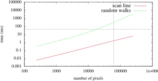
1.5.3.1 Computation time . . . 53
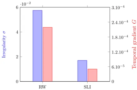
1.5.3.2 Temporal regularity . . . 55
1.6 Conclusion . . . 57
2 Ultrasound-Based Visual Servoing 59 2.1 Visual servoing . . . 60
2.1.1 Introduction . . . 60
2.1.2 Interaction matrix . . . 61
2.1.3 Visual servo control . . . 62
2.1.4 Hybrid tasks . . . 64
2.2 Ultrasound probe control . . . 65
2.2.1 Notations . . . 68
2.2.2 Geometric visual servoing . . . 68
2.2.2.1 Point-based in-plane control . . . 68
2.2.2.2 3D point-based control . . . 69
2.2.2.3 Moments-based control . . . 70
2.2.3 Intensity-based visual servoing . . . 72
2.2.3.1 Case of a 2D probe . . . 74
2.2.3.2 Case of a 3D probe . . . 75
2.3 Ultrasound-guided needle control . . . 75
2.3.1 Needle steering . . . 76
2.3.2 Path planning . . . 79
2.3.3 Ultrasound-guided needle steering . . . 80
2.3.3.1 2D probe, in-plane needle . . . 80
2.3.3.2 2D probe, out-of-plane needle . . . 81
2.3.3.3 3D probe . . . 81
2.3.3.4 3D US-guided needle steering via visual servoing . . . 81
2.4 Conclusion . . . 86
3 Quality-Driven Visual Servoing 87 3.1 Dynamics of the confidence map . . . 89
3.1.1 General considerations . . . 89
3.1.1.1 Effect of the contact force . . . 89
3.1.1.3 Approximated interaction matrix . . . . 91
3.1.2 Analytic solution for scan line integration . . . 92
3.2 Geometric confidence features . . . 95
3.2.1 2D Case . . . 95
3.2.1.1 Definition . . . 95
3.2.1.2 Experimental comparison . . . 96
3.2.1.3 Feature dynamics . . . 97
3.2.2 3D Case . . . 100
3.3 Global confidence-driven control . . . 101
3.3.1 Force control . . . 102
3.3.2 Confidence control . . . 106
3.3.3 Tertiary task . . . 107
3.4 Target-specific confidence-driven control . . . 108
3.4.1 Target centering . . . 109 3.4.2 Confidence control . . . 111 3.5 Conclusion . . . 113 4 Experimental Results 115 4.1 Experimental setup . . . 115 4.1.1 Equipment . . . 116 4.1.1.1 Ultrasound systems . . . 117 4.1.1.2 Robots . . . 118 4.1.1.3 Phantoms . . . 118 4.1.2 Implementation details . . . 119 4.2 Convergence analysis . . . 119
4.2.1 Global confidence control . . . 120
4.2.2 Target-specific confidence control . . . 122
4.3 Reaction to disturbances . . . 126
4.3.1 Global confidence-driven control . . . 126
4.3.2 Target-specific confidence-driven control . . . 128
4.3.2.1 Evaluation of target tracking quality . . 131
4.4 Confidence-optimized tele-echography . . . 133 4.4.1 Phantom experiment . . . 133 4.4.2 In vivo experiment . . . 136 4.5 Conclusion . . . 139 Conclusion 143 List of Publications 151
Bibliography 157
List of Figures 179
Introduction
Medical imaging has been one of the most important revolutions in health care. Indeed, visualizing the interior of the body without the need to open it has enabled a change of paradigm for medical diagnosis. First, because until the end of the nineteenth century, seeing and analyzing the inside of the human body required to perform an open surgery. Open surgery leaves large wounds on the body, which can be painful, and heal slowly with a risk of infection. In this regard, medical imaging enables noninva-sive diagnosis as well as minimally invanoninva-sive procedures, where only a small incision is made in order to insert a surgical tool. Second, because medi-cal imaging provides a way to visualize any part of the human body in its functional state. The advent of medical imaging dates back to the discov-ery of X-rays by Wilhelm Röntgen in 1895. Noticing the surprising prop-erties of these rays capable of propagating through opaque media, Rönt-gen had the idea to experiment it on the human body [RöntRönt-gen, 1898]. One of the first pictures, now famous, produced with his system displays the left hand of his wife. Since then, medical imaging has been contin-uously improved, with the development of Computerized Tomography (CT) by Allan McLeod Cormack and Godfrey Hounsfield [Hounsfield, 1973], and Magnetic Resonance imaging (MRI) by Paul Lauterbur and Peter Mansfield [Lauterbur, 1973; Mansfield, 1977].
Medical ultrasound (US) imaging, based on the propagation of ul-trasonic waves in the body, was also developed in the same period. In contrast with other imaging modalities, ultrasonography provides real-time imaging capabilities. Consequently, ultrasound is the modality of choice for imaging moving organs, such as in echocardiography, and for intraoperative imaging. Ultrasound is also harmless, unlike X-ray imag-ing, which emits ionizing radiations [Frush, 2004]. Moreover, ultrasound imaging devices are lightweight and inexpensive compared to a CT or MRI scanner. This is another advantage for its use in an operating room. However, the clinical use of ultrasound has developed quite slowly compared to radiology, and was, until recently, quite marginal. An ex-planation for this relatively poor use of ultrasound was the low quality of
the images it produces, together with the limited field of view it provides. With the recent technological improvements on the design of ultrasound transducers, the quality of ultrasound imaging has increased steadily. In addition, an ever greater importance is given to the cost effectiveness of medical procedures. For these reasons, ultrasound is now recommended as a frontline imaging modality for more and more applications. However, clinical assessment based on free-hand ultrasound imaging is subject to a large inter- and intraoperator variability. The frequent manual manipu-lation of an ultrasound probe is also a source of musculoskeletal disorders for sonographers. Consequently, robotized ultrasonography is emerging as a solution to assist the sonographer and to improve the reliability and repeatability of examinations and surgical procedures.
Despite the potential benefits that medical robotics can bring to a wide range of medical procedures, the introduction of robotic systems into the clinic has been quite limited, compared to the rapid develop-ment of robotics in the industrial sector. A reason for the relatively slow development of medical robots is the complexity of operative procedures, where the robot has to interact safely and transparently with the med-ical staff and the patient. [Navab et al., 2016] discuss the requirements for intraoperative imaging systems, and retain the criteria of relevance, speed, flexibility, usability, reliability, reproducibility, and safety. These are all critical requirements that have to be met for a robotic system to be accepted in the operating room. In particular, the purpose of a medi-cal robot should not be to replace the surgeon. It should rather serve as a tool, among others, to assist him during the medical procedure. In this regard, it is important to integrate a medical robotic system as a com-ponent of a global Computer-Integrated Surgery (CIS) workflow [Taylor and Stoianovici, 2003].
Due to its real-time imaging capability, ultrasound is a modality of choice for robot-assisted medical procedures. Indeed, real-time ultra-sound feedback can provide the system with the flexibility and reactivity required to perform personalized and adaptive procedures. Flexibility is crucial in intraoperative imaging in order to adjust the procedure to the characteristics of each patient. Reactivity should allow the system to adapt dynamically to the surgeon’s commands, but also to the cur-rent state of the process. In this regard, intraoperative ultrasound can provide precious information on the patient. It can be used to adapt the process by taking into account, for instance, patient motion or organ de-formation. This contrasts with procedures based on preoperative imaging alone, where the surgeon cannot observe the current state of the body. Thus, robot-assisted systems with ultrasound guidance are promising for a wide range of clinical applications.
Clinical motivations
Teleoperated diagnostic ultrasound
The idea of tele-echography (or teleultrasound) has emerged at the end of the twentieth century as a solution to enable remote expert clinical diagnosis [Sublett et al., 1995; Coleman et al., 1996]. The motivation behind the development of telemedicine is twofold. First, the accessibil-ity to qualaccessibil-ity health care is unequally distributed. Specialists tend to be located in highly populated areas, whereas rural and remote regions have only access to minimal, if any, medical care. Thus, telemedicine is a low cost solution to increase the accessibility to high-standard medical care. Second, regular visits to remote hospitals can be exhausting for patients. For instance, patients under long-term hemodialysis need to be checked regularly for amyloid arthropathy. In this context, tele-echography has the potential to provide expert diagnosis in a local hospital with limited resources, or even at home. Tele-echography initially relied on a video conferencing system. Video communication allowed an expert to perform a diagnosis remotely, with the help of a technician on site [Kontaxakis et al., 2000]. With a teleoperated robotic ultrasound system, the expert clinician can manipulate the ultrasound probe himself [Vilchis et al., 2003; Arbeille et al., 2003; Courreges et al., 2004]. Teleoperated ultra-sound has been considered for the examination of arteries [Pierrot et al., 1999; Abolmaesumi et al., 2002], in obstetrics [Arbeille et al., 2005], and in echocardiography [Boman et al., 2009].
Interventional imaging
Prostate cancer biopsy
Prostate cancer is the second most frequent cancer in men in the world, and the most frequent in occidental countries [Brody, 2015]. When sus-pected, prostate cancer is typically diagnosed by performing a biopsy, which consists in the insertion of a needle to extract tissue samples to be analyzed. Prostate cancer biopsy is most commonly conducted under Transrectal Ultrasound (TRUS) guidance to allow for a precise position-ing of the needle. However, the quality of the biopsy under freehand TRUS is dependent on the clinician’s expertise. The use of a robotic system in this context has several advantages, which are discussed, e.g., in [Kaye et al., 2014]. For instance, the needle can be automatically aligned with the target to allow for a greater precision, by accounting for tissue displacement. It has been demonstrated that robot-assisted
TRUS biopsy can improve the cancer detection rate, compared to free-hand TRUS biospies [Han et al., 2012].
Brachytherapy
Brachytherapy consists in the implantation of radioactive seeds at a pre-cise location for the treatment of cancer. As for biopsies, brachytherapy is most frequently performed under TRUS guidance. Therefore, robotic systems can assist in the placement of the probe, tracking of the target and needle, as well as needle placement [Wei et al., 2005; Fichtinger et al., 2008].
Laparoscopic prostatectomy
Robotic systems are also used for laparoscopic prostatectomy (prostate removal). In this context, intraoperative TRUS imaging is required in order to visualize neurovascular bundles that have to be preserved [Long et al., 2012; Hung et al., 2012].
Breast cancer biopsy
Breast cancer is one of the first causes of cancer-related death in women, with about 500 000 deaths each year worldwide [Stewart and Wild, 2014]. Breast biopsy is the standard protocol for cancer diagnosis. Ultrasound guidance is widely used for breast biopsy, because it provides a real-time visualization of the target, which can be displaced due to the insertion of the needle. However, freehand ultrasound-guided biopsy is strongly dependent on the expertise of the clinician. Therefore, a robotic system can assist in breast biopsy for needle placement [Kobayashi et al., 2012] or tissue stabilization [Mallapragada et al., 2011; Wojcinski et al., 2011]. High intensity focused ultrasound
High Intensity Focused Ultrasound (HIFU) is an emerging method for tumor ablation. Based on the generation of focalized ultrasound to gen-erate a local thermal lesion, HIFU therapy is a promising technology, because it is minimally invasive [Tempany et al., 2011]. Robotic HIFU was proposed early for the placement of the robotic transducer in neu-rosurgery [Davies et al., 1998]. However, HIFU therapy based on pre-operative planning has a limited precision, due to registration errors and tissue displacements. Recently, closed-loop robot-assisted HIFU was con-sidered to allow for motion compensation using ultrasound-based visual servoing [Seo et al., 2011; Chanel et al., 2015].
Challenges
Several challenges are associated to the design of robotic ultrasound sys-tems. We detail thereafter the main challenges in terms of image analysis, real-time requirements, modeling, and image quality.
Image analysis First, a reactive robotic ultrasound system should be able to exploit the information available in the ultrasound images. The noisy nature of ultrasound images can make this task extremely difficult, compared to other imaging modalities. As a result, the analysis of ultra-sound images, which comprises segmentation, tracking, registration, and feature extraction, is a whole field of research by itself.
Speed Robotized ultrasound brings an additional constraint to the de-sign of image processing algorithms, in terms of real-time requirements. Indeed, the processing of the images should be fast enough to enable a close-loop control of the robot. In the image processing literature, the term real-time is often used loosely, to indicate that a process is fast enough to allow interaction with a human. It is important, however, to always look at the targeted application before to consider a process as real-time. An acceptable definition would be that a real-time system is able to process information at the same rate as the said information is produced. In ultrasound-guided robotics, a real-time system should also allow a reactive control of the robot. As a result, while many elabo-rated ultrasound image analysis methods are available, the priority in ultrasound-guided robotics is the speed and the robustness of the algo-rithms.
Interaction modeling Controlling a robot under ultrasound guidance requires a model of the interaction between the motion of the robot and the image contents. While efficient solutions exist for image-guided con-trol, and, in particular, visual servoing, the characteristics of ultrasound imaging makes the modeling of interactions more difficult. Specific chal-lenges are the noise of the images, tissue deformations, but also the fact that 2D ultrasound probes only provide information in their observation plane.
Image quality Finally, the quality of ultrasound images depends on several factors, which are not always controlled. In particular, ultrasound image quality depends on the acoustic coupling between the probe and the patient’s skin. For this reason, the use of acoustic gel and the contact
force with the body are crucial factors of image quality. Moreover, the position and orientation of the probe with respect to the tissues influ-ences the quality of the ultrasound signal. Indeed, the intensity of the ultrasound echo depends on the path traveled by the wave to reach a certain point and to propagate back to the transducer. The amplitude of the sound signal can decrease drastically when there are strong changes in acoustic impedance, such as at tissue/bone or tissue/gas interfaces. Consequently, the ultrasound signal quality can be highly heterogeneous within the image, and it is important to position the probe on a good acoustic window in order to have a clear image of the target anatomy. In ultrasound-based visual servoing, the impact of probe positioning on the image quality is usually ignored. As a result, the visibility of the target is not guaranteed.
Context and objectives
This thesis was conducted in a co-supervision scheme between the La-gadic team at IRISA, Université de Rennes 1 and the CAMP group at the Technische Universität München. Starting from the observation that ultrasound image quality has received little attention, the purpose of this thesis was to investigate the possibility to optimize the quality of ultra-sound acquisitions via a dedicated control strategy. Thus, the aim of this thesis was to answer the questions:
• How can one represent the quality of the ultrasound signal?
• How can one control the position of an ultrasound probe so as to maximize the quality of acquired images?
Contributions
The main contributions of this thesis are:
• A method for tracking a flexible biopsy needle in 3D ultrasound images.
• A new method for estimating the quality of the acoustic signal in ultrasound images. This method, based on an integration of the ultrasound signal along the scan lines, provides a real-time pixel-wise estimation of image quality.
• A comparison between this new quality estimation method and an existing method based on the random walks algorithm, in terms of computational cost and regularity.
• A study of the relation between the position of an ultrasound probe and the distribution of the ultrasound signal quality within the image.
• The use of the ultrasound confidence map as a visual modality to perform a closed-loop control of a robot-held probe. Control strate-gies are proposed for optimizing the image quality either globally, or with respect to a specific anatomic target. This contribution addresses the different challenges described above, in particular in terms of modeling and real-time processing requirements.
• A control fusion approach, to combine the proposed quality-driven control with other tasks, such as force control and target tracking. • A validation of the proposed methods via experiments which
illus-trate different use cases.
The contributions on the topic of quality-driven control were partly published in two articles in the proceedings of the International con-ference on Robotics and Automation (ICRA) [Chatelain et al., 2015b, 2016]. The contribution on the tracking of a flexible biopsy needle under 3D ultrasound guidance was also published in an ICRA paper [Chatelain et al., 2015a].
During the preparation of this thesis, other contributions were made that are not discussed herein, because they are out of the topic of this dissertation. We provide the abstracts of the corresponding publications in the appendix.
Thesis outline
This manuscript is organized as follows.
Chapter 1 We present an overview of ultrasound image analysis tech-niques. The chapter starts with an introduction to ultrasound imaging, which provides a basic background on this imaging modality. Then, we present a review of ultrasound image analysis algorithms, focusing on soft tissue and instrument tracking methods with real-time capability. In this context, we provide a first personal contribution on the tracking
of a flexible needle in 3D ultrasound images. Finally, we introduce dif-ferent methods for the estimation of ultrasound signal quality, and we propose a new algorithm that presents some advantages compared to the state of the art.
Chapter 2 We address the topic of ultrasound-guided robot control, with a particular focus on ultrasound-based visual servoing methods. Af-ter a general introduction to visual servoing, we provide a review of the state-of-the-art on (i) methods for controlling an ultrasound probe, and (ii) methods for controlling a surgical instrument, under ultrasound guid-ance. We also propose a personal contribution on this second topic, which consists in a 3D ultrasound-based visual servoing method for steering a flexible needle.
Chapter 3 We present the main contribution of this thesis. Based on the notions introduced in the two previous chapters, we propose a model of the interaction between the probe positioning and the quality of ultrasound images. Then, we use this model to design different control approaches aimed at optimizing the quality of ultrasound imaging. Chapter 4 We provide experimental results which validate the frame-work introduced in chapter 3. We illustrate the application of our method to a teleoperation scenario, with a shared control between the automatic controller and a human operator. In particular, we provide the results of experiments performed with our framework on a human subject.
Conclusion Finally, we draw the conclusions of this dissertation, and we propose perspectives for further developments.
Chapter 1
Ultrasound Image Analysis
This chapter provides an overview of ultrasound image analysis methods. The automatic processing of ultrasound images, ranging from low-level signal processing to computer-aided diagnosis, provides ways to improve the image quality, to assist the physician in interpreting the images, and to extract quantitative clinical features that are valuable for diagnosis or treatment planning. While physicians are well trained in the inter-pretation of ultrasound images, computer-aided analysis is desirable to perform tedious and time-consuming tasks, such as segmentation or reg-istration. In addition, modern ultrasound technologies such as three-dimensional ultrasound and elastography generate data that are more challenging to analyze than conventional B-mode ultrasound. The anal-ysis of ultrasound images is also subject to inter- and intra-observer vari-ability [Tong et al., 1998]. In this regard, automatic or semi-automatic image analysis can be a tool to help standardizing and improving the reliability of diagnosis and treatment planning. Moreover, automatically interpreting the contents of ultrasound images is necessary to the devel-opment of robot-assisted imaging and ultrasound-guided robotic surgery. In the following, we provide an introduction to ultrasound imaging (section 1.1). Then, we present a review of real-time algorithms for soft tissue tracking (section 1.2) and needle tracking (section 1.3). On this topic, we propose a new solution for tracking flexible needles in 3D ul-trasound via particle filtering (section 1.4). Finally, we address the issue of estimating the quality of ultrasound images (section 1.5).
1.1
Ultrasound imaging
1.1.1
Piezoelectricity
The development of ultrasound imaging was enabled by the discovery of the piezoelectric effect at the end of the 19th century. Piezoelectricity was first evidenced by the brothers Jacques and Pierre Curie, who ob-served a production of electricity in hemihedral crystals, induced by me-chanical compression and decompression [Curie and Curie, 1880]. This phenomenon is analogous to another property of these crystals which was already well known at this time: the production of electricity by a change of temperature, or pyroelectricity. In 1881, Lippmann predicted, through his analytic formulation of the electricity conservation law, that the reverse effect should also occur. That is, a hemihedral crystal would deform under the action of electricity [Lippmann, 1881]. The reverse piezoelectric effect was confirmed experimentally in the same year by the Curie brothers [Curie and Curie, 1881].
One of the first notable applications of piezoelectricity was an ul-trasonic underwater detector for submarines [Chilowsky and Langevin, 1916]. Therapeutic applications of ultrasound were investigated in the middle of the 20th century, with, for example, the work of [Bierman, 1954] on the treatment of scars. A first attempt of application to diag-nostic ultrasound imaging was made by [Dussik, 1942]. Dussik proposed an imaging system based on the transmission of ultrasound between an emitter and a receiver, and presented an image resulting from the scan of a brain. However, the structures appearing in the image were, in fact, imaging artifacts due to reflections of the skull [Güttner et al., 1952]. The first successful ultrasound diagnosis experiments are due to Lud-wig and Struthers, who reported the detection of gallstones in biological tissues [Ludwig and Struthers, 1949].
[Wild and Reid, 1952] combined a piezoelectric transducer with a mechanical scanning system in order to create a two-dimensional ultra-sound image. This invention has led to what is now known as B-mode ultrasound imaging. B-mode imaging has been later improved by [Howry et al., 1955], who evidenced the presence of ultrasonic interfaces between different tissues.
1.1.2
Ultrasound image formation
1.1.2.1 Ultrasound propagation
Sound is a mechanical wave of pressure and displacement that propagates through a medium. The human ear is sensible to sound with frequencies
between 20 Hz and 20 kHz [Davis, 2007]. Ultrasound is a sound wave with frequency higher than 20 kHz, i.e., beyond the audible limit of humans. Conventional medical ultrasound systems operate in the range between 1 MHz and 20 MHz [Chan and Perlas, 2011].
The speed of sound depends on the properties of the medium it propa-gates through. It can be described by the Newton-Laplace equation [Biot, 1802]
c = �
K
ρ, (1.1)
where c is the speed of sound, K is the bulk modulus (a coefficient of stiffness) of the medium, and ρ is the density of the medium. Thus, the speed of sound increases with the stiffness of the tissues, and decreases with the density. The speed of sound is also related to the frequency f and the wavelength λ by
c = f λ, (1.2)
so that the wavelength is inversely proportional to the frequency. Since the wavelength indicates the resolution at which adjacent objects can be distinguished, the axial resolution of ultrasound images is proportional to the frequency. For this reason, superficial structures are imaged at high frequencies (from 7 MHz to 20 MHz), while deeper structures are imaged at lower frequencies (from 1 MHz to 6 MHz) to allow for a greater pen-etration, at the cost of a lower resolution. The speed of sound in soft tissues is generally assumed to be constant at 1540 m s−1. Thus, the
wavelength for medical ultrasound lies between 77 µm (at 20 MHz) and 1.54 mm (at 1 MHz). Therefore, ultrasound imaging has the capability to distinguish structures at a submillimeter accuracy. This high resolu-tion is, together with the real-time imaging capability, one of the main advantages of ultrasound, compared to other medical imaging modalities. When traveling through the tissues, ultrasound is subject to reflec-tions at tissue interfaces. Assuming that the ultrasound wavelength is small with respect to the structure, the interaction at a boundary be-tween two media with different acoustic properties can be described with Snell’s law, which links the incidence, reflection and transmission direc-tions to the acoustic velocity in the two media. Let us consider a medium 1 with sound velocity c1, a medium 2 with sound velocity c2, and a sound
wave hitting the interface with an incidence angle θi with respect to the
normal to the interface (see Figure 1.1). When θi �= 0, the direction of
incidence and the normal to the interface define a plane, which is referred to as the plane of incidence. Snell’s law states that the sound wave is reflected (resp. transmitted) in the plane of incidence with an angle θr
c1 c1 c2 θi θr θt Medium 1 Medium 2
Figure 1.1 – Specular reflection and transmission of a sound wave at an interface between two media.
(resp. θt), such that
sin θi c1 = sin θr c1 = sin θt c2 . (1.3)
In particular, when an ultrasonic wave intersects a tissue boundary at normal incidence, part of the wave is reflected directly in the opposite direction. This is one of the most important phenomena underlying the formation of ultrasound images, as the reflected echo indicates the pres-ence of a tissue boundary. At non-normal incidpres-ence angles, however, the ultrasound is reflected away from the source.
When the ultrasound wave encounters objects with a scale that is comparable to or smaller than its wavelength, the wave is reflected in all directions. This phenomenon is referred to as scattering, or diffuse reflection, as opposed to specular reflection. Scattering is responsible for the texture patterns characterizing ultrasound images. It is also one of the sources of energy loss for the sound wave.
Soft tissues also have a certain viscosity, which causes the conversion of acoustic energy to thermal or chemical energy. Therefore, part of the energy of the ultrasound wave is absorbed by soft tissues and converted to heat. Acoustic attenuation in soft tissues can be expressed as a frequency-dependent power law [Wells, 1975]
p(x + δx) = p(x)e−αδx, (1.4)
where p is the sound pressure amplitude, x is the position, δx is the displacement, and α is a frequency-dependent attenuation coefficient. 1.1.2.2 Radio frequency ultrasound
Ultrasound transducers consist in an array of piezoelectric crystals, with typically 128 elements. The piezoelectric elements can be triggered by an
D E L A Y C O N V O L U T IO N pulse carrier focus point
Figure 1.2 – Generation of a focused ultrasound beam. A Gaussian pulse is modulated by a sinusoidal carrier to produce a pulse wave. The transmission pulse is delayed and sent to trigger an array of piezoelectric crystals.
electric signal to generate an ultrasound wave by vibration of the crystal. In practice, a small group of adjacent elements is triggered synchronously, each with a specific time delay, in order to generate a focused ultrasound beam. The electric signal applied to the transducer elements consists in a sinusoidal wave convolved with a Gaussian modulator, in order to generate a pulse. This ultrasound beam generation process is illustrated in Figure 1.2.
Conversely, the transducer elements allow the reception of reflected ultrasound echoes. The returning ultrasound wave triggers the crystals, which, in turn, generate an electric signal. Thus, the acquisition of a scan line consists in a transmission phase, where an ultrasound pulse is generated, and a listening phase, where the returning signal is processed. The listening phase lasts for a predefined period of time, which depends on the desired imaging depth. Indeed, imaging at a depth d requires to listen for a time
T = 2d
c , (1.5)
where c is the speed of sound. For instance, the acquisition of a scan line at a depth d = 10 cm, assuming a speed of sound c = 1540 m.s−1,
requires to listen to the echo during T ≈ 0.13 ms.
The signal received during the listening phase is then amplified, and compensated for attenuation by a time gain compensation function, i.e., a depth-dependent gain adjustment. The resulting signal is referred to as the radio frequency (RF) signal. An example of RF line measure is shown in Figure 1.3.
The acquired RF signal takes the form
u(t) = A(t) cos(2πfct + φ(t)), (1.6)
0 0.02 0.04 0.06 0.08 0.1 0.12 0.14 0.16 0.18 0.2 RF intensity u (t ) time t (ms)
Figure 1.3 – Radio frequency ultrasound signal.
function. Alternatively, to simplify subsequent mathematical manipula-tions, the RF signal can be expressed in its analytic form
z(t) = u(t) + jH(u)(t), (1.7) where H(·)(t) is the Hilbert transform, defined as
H(u)(t) =−1 πlim�→0 � ∞ � u(t + τ )− u(t − τ) τ dτ. (1.8) In practice, the Hilbert transform of the signal is computed in the Fourier domain.
RF demodulation consists in extracting the signal envelope, by re-moving the sinusoidal carrier component. This processing step can be performed by computing the module of the analytic signal, defined as
Uenv =
�
u(t)2+ H(u)(t)2, (1.9)
which is referred to as the envelope-detected RF signal. Figure 1.4 shows the envelope-detected signal computed from the RF line of Figure 1.3.
The RF signal is sampled at the sampling frequency fs. Following
the Nyquist criterion, the sampling frequency guarantees a perfect re-construction of the signal if it satisfies the inequality
fs > 2fmax, (1.10)
where fmax is the highest frequency of the signal [Shannon, 1949]. The
sampling frequency is typically set to 20 MHz for convex probes, which work at frequencies below 10 MHz, and to 40 MHz for linear probes, which use higher frequencies up to 20 MHz.
Given a sampling frequency fs, an acquisition up to depth d provides
ns=
fsd
0 0.02 0.04 0.06 0.08 0.1 0.12 0.14 0.16 0.18 0.2 RF en v elope Ue n v (t ) time t (ms)
Figure 1.4 – Envelope-detected ultrasound signal.
samples. For instance, sampling at depth d = 10 cm with frequency fs = 40 MHz provides ns = 2597 samples. This number is larger than
necessary for display. For this reason, the envelope detected RF signal is usually decimated, that is, subsampled by a factor 10. We define
fA =
fs
10 (1.12)
the A-sample frequency. This corresponds to the final sampling fre-quency. Note that decimation is done after envelope-detection, so that the Nyquist criterion is respected for the envelope-detection. Then, the number of A-samples in a scan line is
AN = ns 10 =
fAd
c . (1.13)
1.1.2.3 B-mode ultrasound
Envelope detected RF data is conventionally represented numerically by 16-bits integers. Therefore, the dynamic range has to be reduced to 8-bits for display. In order to preserve low-intensity values, dynamic range compression is typically done by a non-linear mapping, such as the logarithmic compression
flog(x) = A log(x) + B, (1.14)
or the square-root operator
fsqrt(x) = Ax0.5+ B, (1.15)
where A is the amplification parameter, and B is a linear gain parameter. For the acquisition of a 2D section, the same procedure is repeated for each transducer element, which results in a set of LN (line number)
scan lines. A typical line number, found in most of the commercial transducers, is LN = 128. Note that, following the previous example of a scan line acquisition lasting for 130 µs, the acquisition of a 2D section will take about 17 ms, so that the frame rate of B-mode ultrasound, with these settings, is f2D ≈ 60 Hz. This frame rate is higher than necessary
to provide a fluid display to the user. As a result, B-mode ultrasound is considered as a real-time imaging modality.
Ultrasound probes come in different shapes to fit various medical purposes. The transducer geometries can be roughly categorized in two sets. In linear probes, the transducer elements are aligned, and the scan lines are parallel. In convex (or curved) probes, the transducer elements are placed along a circular arc, and the scan line are fan-shaped. In both cases, the scan lines are coplanar. Objects and directions contained in the plane defined by the scan lines is referred to as in-plane, while objects and directions not contained in that plane are referred to as out-of-plane. In the following, we detail the imaging geometry of linear and convex probes.
Linear probes For linear probes, the scan lines are parallel, and the imaging region is rectangular, as represented in Figure 1.5. Therefore, the processed scan lines can be directly aggregated to form the B-mode image. The relation between a physical point located at (x, y) in the field of view and a pixel (i, j) in the image is given by
x = Lpitch× (j − j0), (1.16)
y = Apitch× i, (1.17)
where Apitch is the A-pitch, or axial resolution, defined as the distance
between two consecutive samples along a scan line. Given the A-sample frequency fA, the A-pitch can be computed as
Apitch =
c fA
. (1.18)
Similarly, the L-pitch Lpitch is defined as the distance between two
consecutive transducer elements.
Convex probes For convex probes, however, the imaging region is a fan-shaped sector, and the conversion to B-mode requires a geometrical conversion from polar to Cartesian coordinates, which is referred to as scan conversion. Following the notations of Figure 1.6, let Fp be the
frame attached to the imaging center O of the probe, such that the x-y plane coincides with the imaging plane, and the x-y direction passes
Field of view y x i j j 0 Image Figure 1.5 – Geometry of a 2D linear ultrasound probe.
Field of view θ r rmin rmax θmin Θ θmax y x Fp O x y Fp O θ j i ymin ymax xmin xmax
Figure 1.6 – Geometry of a 2D convex ultrasound probe.
through the center of the imaging sector. In polar coordinates, we note r the distance to O, and θ the angle with respect to the y-axis. The polar and Cartesian coordinates are related by the equations
x = r sin θ, (1.19) y = r cos θ. (1.20) Let l be the scan line index, and a the sample index along each scan line, in the order of acquisition, starting from 0. We write rmin the probe
radius, i.e., the distance from the imaging center to the first sample. Similarly, we define rmax as the distance from the imaging center to the
farthest sample. Under the assumption of a constant velocity of sound c, the a-th sample in each scan line corresponds to the echo produced by the tissue element located at a distance
r = rmin+ Apitcha, (1.21)
where the A-pitch Apitch is defined as in (1.18).
Knowing the L-pitch (distance between two adjacent transducer el-ements) Lpitch and the probe radius rmin, one can compute the angular
resolution
δθ= Lpitch rmin
, (1.22)
and the angular field of view
Θ= LN δθ. (1.23) Then, noting θmin =−Θ2 and θmax = Θ2 the limits of the angular field of
view, the angular position of the l-th scan line can be computed as θ= θmin+ lδθ. (1.24)
The B-mode image, with pixels indexed by (i, j), can be reconstructed at an arbitrary resolution s with
i = y− ymin
s , (1.25)
j = x− xmin
s , (1.26)
where xmin and ymin are the smallest x- and y- coordinates of the field of
view, respectively. These values can be easily computed as
xmin = rmaxsin θmin, (1.27)
and
ymin = rmincos θmin. (1.28)
Finally, the B-mode image is constructed by interpolating for each (i, j) the prescan image at
a = �
(rmaxsin θmin+ s.j)2+ (rmincos θmin+ s.i)2− rmin
Apitch
(1.29) l = arctan
rmaxsin θmin+s.j
rmincos θmin+s.i − θmin
δθ (1.30)
Different techniques can be used for interpolation:
• Nearest neighbor: the value of the closest prescan data point to (a, l) is used:
Upostscan(i, j) = Uprescan([a], [l]), (1.31)
where [·] is the round to nearest function. This is the simplest and fastest method. However, the resulting image presents undesirable interpolation artifacts.
• Bilinear interpolation: the value of the current pixel is interpolated linearly between the four prescan data points adjacent to (a, l):
Upostscan(i, j) = (l− �l�)U1+ (l− �l�)U2, (1.32)
where �·� and �·� are the round down and round up function, re-spectively,
U1 = (a− �a�)Uprescan(�a�, �l�) + (a − �a�)Uprescan(�a�, �l�), (1.33)
and
U2 = (a− �a�)Uprescan(�a�, �l�) + (a − �a�)Uprescan(�a�, �l�). (1.34)
• Bicubic interpolation: the value of the current pixel is interpolated from 16 neighboring pixels, using Lagrange polynomials or cubic splines. This technique leads to a smoother result, at the cost of a longer processing time.
1.1.2.4 3D ultrasound
Two-dimensional ultrasound probes are limited to the visualization of a planar section of the body, which complicates real-time ultrasound-based diagnosis. First, 2D ultrasound requires expertise to understand and mentally visualize three-dimensional structures of the body. Then, 2D ultrasound does not allow any direct quantitative measurement of anatomical objects or diseases. Finally, for robotic guidance, which is the main topic of this thesis, the lack of information in the out-of-plane direction makes the 3D control of an ultrasound probe challenging.
Three-dimensional ultrasound imaging has been a subject of research since the late 1990s, mainly in the context of obstetrics [Pretorius and Nelson, 1995; Nelson et al., 1996]. Two main 3D ultrasound techniques have been developed and commercialized: motorized transducers and matrix array transducers. We briefly describe these thereafter.
Remark: Volumetric ultrasound imaging is sometimes referred to as 4D ultrasound in the literature. Then, the forth dimension represents the temporal dimension, which is a way to insist on the real-time aspect of ultrasound imaging. In order to avoid any confusion, we reserve in this dissertation the term 2D ultrasound to 2D ultrasound probes, and 3D ultrasound to 3D ultrasound probes.
motor axis x y z Wobbling motion
Figure 1.7 – Geometry of a motorized convex 3D ultrasound probe.
Motorized transducer A motorized 2D transducer, sometimes called wobbler probe, is a 2D transducer that mechanically scans a volume of interest with a back-and-forth motion. The geometry of such a probe is illustrated in Figure 1.7. This system acquires a series of B-mode frames, which can be reconstructed into a volume, based on the known scanning pattern.
Since motorized 3D ultrasound imaging relies on the successive ac-quisition of 2D frames, the 3D acac-quisition rate f3D is at most equal to
the frame rate f2D divided by the number of frames F N:
f3D <
f2D
F N. (1.35)
For instance, for 33 frames per volume, a SonixTOUCH scanner (BK Ultrasound, MA) with the 4DC7-3/40 Convex 4D transducer acquires 1.1 volumes per second. To limit the artifacts due to motion, the sweeping motion has to be slow enough, so as to consider the transducer static during the acquisition of a frame. As a result, the volume rate of such a probe is limited.
Matrix array transducer A more recent design for 3D ultrasound imaging consists in a 2D matrix array of transducer elements, which allows direct volume acquisition [Woo and Roh, 2012]. In this case, the transducer elements are arranged in a 2D regular grid, that can be either planar or bi-convex.
This design alleviates the limitations of motorized scanning, by in-creasing the acquisition speed, while eliminating the artifacts due to the sweeping motion. However, the number of piezoelectric elements em-bedded in matrix array transducers is usually limited, which leads to a relatively low resolution, compared to motorized transducers.
1.2
Soft tissue tracking
The localization of anatomical landmarks is an important step in the analysis of medical images. Automatic segmentation, which consists in delineating the contours of a structure of interest, offers a mean to ease the interpretation of medical images, and to obtain a reliable diagnosis by the direct extraction of quantitative features. In addition,detecting anatomical features in real-time is necessary for the development of in-telligent robot-assisted procedures. Ultrasound image segmentation has been the subject of intensive research for various medical applications [No-ble and Boukerroui, 2006]. Having in mind the context of robotized ul-trasound examination, we focus, in this section, on methods capable of providing real-time tracking, rather than image-by-image segmentation. On the other hand, we do not limit the scope of tracking to the precise delineation of an object’s contour, but we also consider the tracking of a region of interest. Therefore, instead of an exhaustive review of ul-trasound image segmentation techniques, the purpose of this section is to provide an overview of real-time ultrasound tracking algorithms, that can be useful to the design of ultrasound-based robot control strategies.
1.2.1
Motion tracking
1.2.1.1 Block matching
Block matching is a motion estimation technique, that consists in finding corresponding blocks (small regions of interest) between two consecutive images of a sequence. The underlying assumption is that the motion inside each block is rigid, so that pixels contained in a pair of matching blocks have a one-to-one correspondence.
Sliding window Given a block defined in one frame, the localization of the corresponding block in the next frame can be performed by the optimization of a similarity measure with a sliding window approach, as illustrated in Figure 1.8.
For instance, [Trahey et al., 1987] use the B-mode ultrasound intensity correlation as similarity measure to track the motion of speckle pattern
Figure 1.8 – Sliding window approach for block matching.
for blood flow estimation, and [Golemati et al., 2003] use the normalized correlation to track the carotid artery wall. Given two blocks containing N pixels with intensity (I1(i))Ni=1 and (I2(i))Ni=1, the normalized
correla-tion is defined as
ρ(I1, I2) = N
�
i=1
(I1(i)− ¯I1)(I2(i)− ¯I2)
σ(I1)σ(I2)
, (1.36) where ¯· is the mean operator, and σ(·) is the standard deviation. The normalized correlation ρ takes values in the interval [−1, 1], where ρ = 1 corresponds to a perfect correlation (I1 = kI2, where k is a positive
scalar), ρ = 0 denotes a total decorrelation, and ρ = −1 denotes a perfect anti-correlation (I1 = kI2, where k is a negative scalar). Due to
the normalization by the standard deviation of the signals, this similarity measure is independent of global intensity variations.
Other similarity measures used for block matching in ultrasound im-ages, and inspired from the computer vision community, include the sum of absolute differences [Bohs and Trahey, 1991], and the sum of squared differences (SSD) [Yeung et al., 1998; Ortmaier et al., 2005; Zahnd et al., 2011]. A review and comparison of block matching algorithms for ultra-sound images can be found in [Golemati et al., 2012].
In addition to generic similarity measures, some authors have also de-signed ultrasound-specific similarity measures, in order to better model the specificities of the ultrasound signal. [Cohen and Dinstein, 2002] and [Boukerroui et al., 2003] use the Rayleigh distribution to model the speckle noise statistics. This model is used for speckle tracking in 3D echocardiography in [Song et al., 2007] and [Linguraru et al., 2008]. [My-ronenko et al., 2009] introduce similarity measures based on the bivariate Rayleigh and the Nakagami distributions. A Nakagami-based similarity measure is used in [Wachinger et al., 2012].
Figure 1.9 – Gauss-Newton optimization approach for block matching.
Instead of an exhaustive sliding window search, the optimization can be performed in a neighborhood around the previous block location, when a bound on the displacement is known. Reducing the search space has the double advantage to reduce the computational cost, and to limit the risk of mismatch with similar patterns at other locations.
However, the sliding window approach is limited to the tracking of pure translation motion. To account for a rotation of the target, it is necessary to optimize the orientation of the Region of Interest (ROI) as well. An exhaustive search for the orientation can become computation-ally costly, especicomputation-ally in 3D, so that smarter optimization approaches should be considered.
Gauss-Newton optimization [Hager and Belhumeur, 1998] describe a linear optimization approach based on the Gauss-Newton algorithm. This method is used in [Krupa et al., 2009] and [Nadeau et al., 2015] to track a region of interest in 2D and 3D ultrasound, respectively. It consists in iteratively updating the position of the ROI to converge to-wards a position that minimizes the difference with the initial template, as illustrated in Figure 1.9.
Let I : Ω −→ R represent the ultrasound image where the template is searched for, and P a point with coordinates (x, y, z) in a frame at-tached to the ROI R. The pose of the ROI is represented by a vector of parameters r = (tx, ty, ty, θux, θuy, θuz), encoding its position and
ori-entation with respect to the image frame. Here, the terms (tx, ty, tz)
correspond the translation between the image frame and the ROI frame, and (θux, θuy, θuz) correspond the axis-angle representation of the
rota-tion between these frames. The variarota-tion of the intensity IP at P can be
related to the displacement of the ROI by an interaction matrix LIP = ∂IP
which can be written LIP = � ∂IP ∂P �� ∂P ∂r, (1.38)
where the first term corresponds to the 3D image gradient ∂IP
∂P = �
∇Ix ∇Iy ∇Iz
�
. (1.39)
The second term is given by Varignon’s formula for velocity composition: ∂P ∂r = 1 0 00 1 0 −z0 z0 −yx 0 0 1 y −x 0 , (1.40) so that the interaction matrix LIP takes the form
LIP = [ ∇Ix ∇Iy ∇Iz
y∇Iz− z∇Iy −x∇Iz+ z∇Ix x∇Iy− y∇Iz ]. (1.41)
The intensity pattern inside the region R can be represented by a vector sR of pixel intensities interpolated on a regular grid G(R):
sR= (IP)P∈G(R), (1.42)
and the interaction matrix for this vector is obtained by stacking the interaction matrices associated to all points in G(R):
LsR = LIP1 ... LI PN , (1.43)
where N is the size of sR.
Noting s∗
R the reference template, the optimization process aims at
minimizing the sum of squared errors SSE(sR, s∗R) =
N
�
i=1
(sR− s∗R)2. (1.44)
The Gauss-Newton algorithm performs the least squares optimization iteratively, with updates
δr=−L+sR(sR− s
∗
R), (1.45)
where L+
sR is the Moore-Penrose pseudoinverse of LsR, defined as
L+sR =�L�sRLsR
�