HAL Id: hal-02374691
https://hal-mines-albi.archives-ouvertes.fr/hal-02374691
Submitted on 21 Nov 2019
HAL is a multi-disciplinary open access
archive for the deposit and dissemination of
sci-entific research documents, whether they are
pub-lished or not. The documents may come from
teaching and research institutions in France or
abroad, or from public or private research centers.
L’archive ouverte pluridisciplinaire HAL, est
destinée au dépôt et à la diffusion de documents
scientifiques de niveau recherche, publiés ou non,
émanant des établissements d’enseignement et de
recherche français ou étrangers, des laboratoires
publics ou privés.
Automatic inspection of aeronautical mechanical
assemblies using 2D and 3D computer vision
Hamdi Ben Abdallah, Igor Jovančević, Jean-José Orteu, Benoit Dolives,
Ludovic Brèthes
To cite this version:
Hamdi Ben Abdallah, Igor Jovančević, Jean-José Orteu, Benoit Dolives, Ludovic Brèthes.
Auto-matic inspection of aeronautical mechanical assemblies using 2D and 3D computer vision. NDT
AEROSPACE 2019 - 11th Symposium on NDT in Aerospace, Nov 2019, Paris-Saclay, France.
�hal-02374691�
Automatic inspection of aeronautical mechanical assemblies using 2D and 3D
computer vision
Hamdi Ben Abdallah
1,2, Igor Jovanˇcevi´c
2∗, Jean-Jos´e Orteu
1, Benoˆıt Dolives
2, Ludovic Br`ethes
21 Institut Cl´ement Ader (ICA) ; Universit´e de Toulouse ; CNRS, IMT Mines Albi, INSA, UPS, ISAE ;
Campus Jarlard, 81013 Albi, France
2 DIOTASOFT, 201 Rue Pierre et Marie Curie, 31670 Lab`ege, France
*corresponding author, E-mail: ijo@diota.com
Abstract
Quality control is of key importance in the aerospace in-dustry. This paper deals with the automatic inspection of mechanical aeronautical assemblies. For that purpose, we have developed a computer-vision-based system made of a robot equipped with two 2D cameras and a 3D scanner. The 3D CAD model of the mechanical assembly is available. It is used as a reference and it describes the assembly as it should be. The objective is to verify that the mechanical as-sembly conforms with the CAD model. Several types of in-spection are required. For instance, we must check that the needed elements of the assembly are present, and that they have been mounted in the correct position. For this kind of inspection we use the 2D cameras and we have developed inspection solutions based on 2D image analysis. We have found that some types of inspection cannot be performed by using only 2D image analysis. A typical example of such types is detecting the interference between elements. It requires to check if two flexible elements (e.g. cables, harnesses) or a flexible and a rigid element (e.g. pipe, sup-port) are at a safe distance from each other. For this type of situations, we use the 3D data provided by the 3D scan-ner and we have developed an inspection solution based on 3D point cloud analysis. We have also developed a method to compute the best viewpoints for the sensor held by the robot, in order to obtain an optimal view of each compo-nent to be inspected. The view-point selection is performed off-line (before the on-line inspection) and it exploits the CAD model of the mechanical assembly.
The proposed automatic computer-vision-based inspec-tion system has been validated in a context of industrial ap-plications. Our software solution for 2D image analysis has been deployed on the robot platform as well as in a hand-held tablet. Since it requires a 3D sensor, our approach based on 3D point cloud has been tested in the robotic con-text only.
1. Introduction
To automate the inspection process, improve its traceabil-ity and repeatabiltraceabil-ity, and to reduce the human error, many aerospace companies aim to automate numerous and com-plicated operations of quality control of aircraft’s mechani-cal assemblies to address the various and growing security
requirements.
We address the problem of automatic inspection in two parts: first, automatic selection of informative viewpoints before the inspection process is started (offline preparation
of the inspection, section 2), and second, automatic
pro-cessing of the 2D images or 3D point clouds acquired from
said viewpoints (online inspection process, section 3 and
section4).
Several types of verification can be carried out on a me-chanical assembly. For instance, check that the elements of the assembly are present and that they have been mounted in the correct position (the CAD model is the reference), check if two flexible elements (e.g. cables, harnesses) or a flexible and a rigid element (e.g. pipe, support) are at a safe distance from each other, and check that the bend radius of cable complies with safety standards.
According to the type of verification to be performed, one of the two following general strategies has been devel-oped:
1. Model-based 2D image analysis (also called 2D in-spection). This method is easy to deploy since it only uses the two RGB cameras (camera with a wide field of view and camera with a narrow field of view)
mounted on the robot (see Fig.1) and the CAD model
of the object to be inspected. This method is
pre-sented in our recent paper [1].
2. Model-based 3D point cloud analysis (also called 3D inspection). This method uses one RGB cam-era (wide field of view camcam-era) and the 3D scanner mounted on the robot, and the CAD model.
First strategy is preferred whenever possible, for time reasons (3D point cloud acquisition and analysis are more time consuming than those in the case of 2D image).
Rest of the paper is organised as follows. In section2
we present our scoring function for evaluating possible
viewpoints for our inspection tasks. In section 3 our
ap-proach based on 2D image analysis has been detailed and
in section4we explain our methodology based on 3D point
cloud analysis. Finally the paper is concluded in section5.
State of the art in the field is summarized in our recent
pa-pers [1], [2] and [3] so will not be elaborated in the present
3.1.1 Robot-based inspection
Our robot-based inspection platform consists of a mobile robot equipped with three sensors (two cameras and a 3D scanner) mounted on the robot arm end-effector (Fig.4).
Fig 4: Our inspection system: robot with its vision-based sensory system
This setup allows to perform a certain range of actions: (1) localization: a wide field tracking camera allows to precisely localize the effector with respect to the part it controls; (2) inspection: a high-resolution camera with a reduced field of view allows to capture the details and to observe the elements very finely with 7 degrees of freedom; (3) 3D scan: a structured light stereo sensor complements the sensor’s capabilities by digitizing the areas observed; (4) controlling: the whole
10 Vision-based sensory
system
Robot arm with 7 DOF
Mobile platform
Figure 1: Our inspection system: robot with its vision-based sensory system
2. Viewpoints selection: offline process
The initial setup of camera viewpoints cannot be done man-ually, because a human operator cannot define with suffi-cient accuracy the camera position that will allow him to get the best viewpoint of the element to be inspected. There-fore, we need a (semi-)automatic offline configuration pro-cess that is used to compute the best viewpoints which can help to improve the quality and the efficiency of inspection. Later, during the online inspection process, the camera will be placed at those calculated viewpoints.
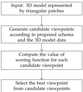
The strategy proposed to find the best viewpoint (com-puting the 6D location – position and orientation – of the camera with respect to the scene to be observed), based on
the 3D model of the assembly is illustrated in Fig. 2. For
each of two types of inspection, a scoring function is con-structed. These functions are designed in a way to maxi-mize observability of the element to be inspected. Finally, the best viewpoint can be selected from all of candidate viewpoints according to the scoring function.
Candidate viewpoints are generated by sampling a fixed radius virtual sphere around the element to be inspected. This radius is chosen in such a manner to comply with dustrial security standards for ensuring security of the in-spected element as well as of the inspecting robot.
The candidate viewpoints are evenly distributed on the sphere surface according the range of longitude θ and
colat-itude ϕ (Fig. 3). The best viewpoint is selected according
to the value of the scoring function.
Version September 13, 2019 submitted to J. Imaging 16 of 28
Input: 3D model represented by triangular patches
Generate candidate viewpoints according to proposed schema
and the 3D model data Compute the value of scoring function for each
candidate viewpoint
Select the best viewpoint from candidate viewpoints
Figure 18.The Overview of Viewpoint Selection Scheme
θ
ϕ
ˆ
x
ˆ
y
ˆ
z = |0i
−ˆ
z = |1i
|V
pointi
ρ
1
Figure 19.A viewpoint on the visibility sphere
The sphere (Fig.20) is defined as a set of viewpoints and the candidate viewpoints are evenly
349
distributed on the sphere surface according the range of longitude θ and colatitude ϕ. 350
Figure 2: The Overview of viewpoint Selection Scheme
θ ϕ ˆ x ˆ y ˆz = |0i −ˆz = |1i |Vpointi ρ 1
Figure 3: A viewpoint on the visibility sphere 2.1. Scoring function for 2D inspection
Our scoring function for 2D inspection combines three cri-teria:
• Visibility of the information (fvisibility)
• Ambiguity of observed shape due to parasite edges (fparasite)
• Similarity of observed shape to expected shape (fshape)
fvisibility - each viewpoint yields a render of our
el-ement of interest with a certain number of pixels. The fvisibility function takes into account this value and
fa-vorizes those viewpoints with higher number of pixels (area in the image). It should be noted that the occlusion is taken
into account in the rendering pipeline (see Fig.6for ex.).
fparasite - this function favorizes the viewpoints with
less rejected edgelets due to parasite edges in their vicinity.
For more details about parasitic edges see section3.4.1.
fshape- finally, each candidate viewpoint is also
evalu-ated by computing the similarity between the shape of fil-tered projected edgelets of the inspection element (obtained
by rejecting those prone to parasitic edges and occlusion) and the unfiltered projected edgelets.
The three criteria presented before for evaluating each
viewpoint are combined using a scoring function fscore:
fscore= wv× fvisibility+ wp× fparasite+ ws× fshape
wv+ wp+ ws= 1
wi’s are weights that assign importances to the different
viewpoint evaluation criteria, and they can be adjusted by the user depending on the importance of the criteria for
a specific inspection application. fvisibility, fparasiteand
fshapeare normalized.
2.2. Scoring function for 3D inspection
For 3D inspection, the scoring function is based on the visi-bility criteria only. This criteria is explained in the previous
section and represented by a function fvisibility. Hence in
the case of 3D inspection the following holds: fscore= fvisibility
3. Inspection by 2D image analysis
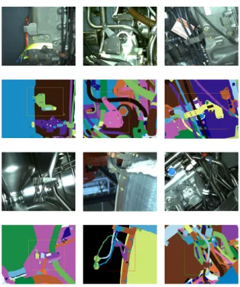
In this section we will detail our main contribution when relying on 2D images and CAD model of the assembly. The goal of this inspection task is to verify that a rigid element of the assembly is present and well mounted. Examples of the CAD models of the assemblies we have been inspecting
can be seen in Fig.4.
Figure 4: Some of our CAD models: (1stcolumn) aircraft
engine, (2nd column) two testing plates with several
ele-ments
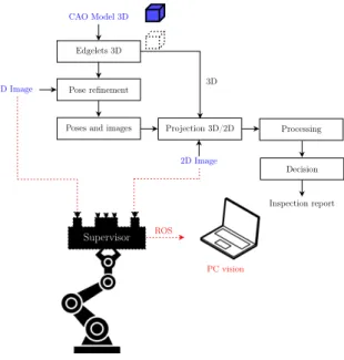
Our inspection process for the defect detection
illus-trated in Fig. 5 consists of four main steps. First, from
the CAD model of the observed object, 3D contour points (edgelets) are extracted. Further, the edgelets with their di-rection vectors are projected onto the real image using a pinhole camera model (extrinsic and intrinsic parameters).
Used image is acquired by the camera with narrow field of view. It should be noted that the pose of the effector is known thanks to the calibration process but also thanks to an in-house developed localisation module which per-forms pose refinement. This module is processing images acquired by the wide field of view camera. Finally, we per-form the matching between the set of projected edgelets and the set of real edges extracted in the image.
We explain each building block of our strategy in the following sections.
Edgelets 3D
Pose refinement
Poses and images Projection 3D/2D Processing
Decision Inspection report 2D Image 2D Image CAO Model 3D 3D Supervisor ROS PC vision
Figure 5: Overview of our online robot-based inspection pipeline
3.1. Step 1 (edgelet generation)
An edgelet Ei is defined as a 3D point pi = (xi, yi, zi)
and a normalized direction vector ~diof the edgelet. These
points pirepresent the 3D contour points of an object (see
Fig.6). The edgelets are extracted offline by rendering a
CAD model as explained in [4].
The output of this step is a set of edgelets that are evenly distributed.
Version October 14, 2019 submitted to J. Imaging 9 of 28
4.1. Step 1 (edgelet generation)
189
An edgelet Eiis defined as a 3D point pi= (xi, yi, zi) and a normalized direction vector ~diof 190
the edgelet. These points pirepresent the 3D contour points of an object, see Fig.8. The edgelets are 191
extracted offline by rendering a CAD model as explained in [22]. The edgelets has been used in other
192
works such as [23–25].
193
The edgelet generation process is well explained in [22]. Loesch et al. [22] introduce an
194
improvement of this process through "dynamic edgelets" extracted online for each point of view.
195
It should be noted that we have opted for using "static edgelets" defined in [22] as edgelets extracted
196
offline using the dihedral angle criteria. The reason being that, as mentioned by [22], the generation
197
of dynamic online edgelets induces an additional computing cost. Moreover, we use the extracted
198
edgelets for generating optimal views in an offline process.
199
• In the case of robot there is no interest for dynamic edgelets, since the point of view is known in
200
advance and there is neither video stream nor tracking as in the case of tablet.
201
• In the case of tablet, we have more severe limitations in computing power so the static edgelets
202
are our first choice for the moment.
203
The output of this step is a set of edgelets that are evenly distributed.
204
(a) (b)
Figure 8.Edgelets extraction: (a) example of CAD part, (b) edgelets extracted from this CAD part
4.2. Step 2 (camera pose estimation)
205
Advantage of our use case is that we dispose of the CAD model of the assembly. Hence, we
206
rely on the work of [22] which combines the edgelet extraction process (described in step1) with a
207
CAD-constrained SLAM algorithm proposed in [26] which is based mainly on [27], the camera being
208
then considered as moving in a partially known environment. The constrained SLAM algorithm
209
accurately estimates the camera’s pose with respect to the object by including the geometric constraints
210
of its CAD model in the SLAM optimization process. In other words, the object is tracked in real time.
211
Our strong pre-assumption is that a moving camera is localized with respect to a complex
212
mechanical assembly. The CAD-based tracking algorithm has been implemented by Diota c and it is 213
used in our work as a black-box that provides us with the required camera pose. More details about
214
this solution will be given in the paper [22].
215
4.3. Step 3 (3D/2D projection)
216
In this phase, we project 3D points of edgelets onto the image using known extrinsic and intrinsic
217
camera parameters (see Fig.9). The input of this step are an image, the camera pose with respect to the
218
assembly (CAD) and a set of evenly distributed edgelets of the element to be inspected.
219
In order to get the camera intrinsic parameters we have used an offline calibration method based
220
on the observation of a classical pattern. Based on various observations of the pattern under different
221
arm configurations we obtained the intrinsic parameters of all the cameras used on the system along
222
with the extrinsic parameters (relative localization) and their absolute localization relatively to the arm
223
Figure 6: Edgelets extraction: (left) example of CAD part, (right) edgelets extracted from this CAD part
3.2. Step 2 (camera pose estimation)
Our strong pre-assumption is that the moving camera is lo-calized with respect to the complex mechanical assembly being inspected. Namely, we rely on an in-house devel-oped system for initial pose estimation based on 2D-3D alignment, our inspection camera being then considered as moving in a partially known environment. The mentioned algorithm accurately estimates the camera’s pose with re-spect to the object by including the geometric constraints of its CAD model in an optimization process.
3.3. Step 3 (3D/2D projection)
In this phase, we project 3D points of edgelets onto the im-age using known extrinsic and intrinsic camera parameters
(see Fig.7). The input of this step are an image, the
cam-era pose with respect to the assembly (CAD) and a set of evenly distributed edgelets of the element to be inspected.
Figure 7: (Left) projection of edgelets (3D points pi),
(right) inward-pointing normals n+i and outward-pointing
normals n−i , generation of search line li
3.4. Step 4 (matching projected edgelets with real edges)
The goal of this step is the matching between the set of projected edgelets and the set of real edges according to the direction of the normal vectors calculated in step 3 (section
3.3). If at least one real edge is found on the search line, the
edgelet is considered matched. Otherwise, it is considered not matched.
Initially we employed the well known and widely used Canny edge detector for extracting meaningful real edges in the real image. The results reported in our recent paper
[1] are obtained by this algorithm.
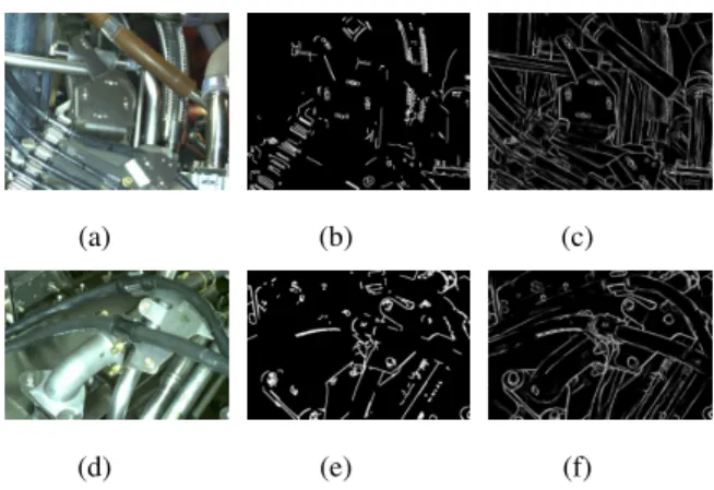
Nevertheless, we have identified more recent edge
de-tection approaches such as [5] based on neural networks.
Fig.8 illustrates a quantitative comparison of Canny edge
detector and the edge detector proposed in [5]. In our
anal-ysis conducted by this moment, we have noticed that the latter one outperforms Canny, notably in treating highly re-flective as well as highly textured areas. Moreover, by us-ing machine learnus-ing based detectors we avoid the sensi-tive phase of parameters tuning unavoidable in the case of Canny approach. In the present paper, the inspection re-sults have been obtained based on 2D edges extracted by the machine learning technique.
(a) (b) (c)
(d) (e) (f)
Figure 8: Quantitative analysis of Canny edge detector and edge detector based on neural network (a,d) input images, (b,e) results by Canny edge detector, (c,f) result by neural network edge detector
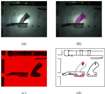
3.4.1. Parasitic edges handling
In this section, we describe our principal contribution, in-troduced in order to remove as much as possible irrelevant edges. Namely, by using CAD render, we anticipate the existence of some portion of parasitic edges coming from other elements mounted in the vicinity of the inspected ele-ment. Indeed, often there are edges very close to the exter-nal boundary of the element to be inspected. We call them
parasitic edges or unwanted (irrelevant) edges. To solve
this kind of problem, we introduce a new notion called
con-text imageof an element to be inspected. From the CAD
data and the particular camera position, we form a synthetic view (context image), which has exactly the same perspec-tive as the real image, only that the inspected element is
excludedfrom the assembly (see Fig.9).
Figure 9: (Left) example of CAD model - inspected element (dark blue) is in the red circle, (right) context image of the inspected element
The process of decreasing number of parasitic edges is
illustrated in Fig.10. First, we project the edgelets of the
element of interest onto the context image, as explained in
step 3 (section3.3).
Further, we form search lines (see Fig.10d) and look
for the intensity change in this virtual context image.
In-tensity changes are shown in Fig.10d. If such a change in
context image is found, it is very probable that this edge will be present in the real image as well. Therefore, we will
not consider this edgelet for matching. These edgelets are
shown in red in Fig.10d. Other edgelets, shown in green in
Fig.10d, are considered in the matching phase.
(a) (b)
(c) (d)
Figure 10: Illustration of the parasitic edges handling: (a) input image, (b) projection of the element to be inspected, (c) context image of the element to be inspected, (d) gra-dient changes in the context image and considered edgelets (green) and rejected edgelets (red)
3.4.2. Edges weighting
For each edgelet in the 3D CAD that is projected onto the image plane, we are interested in finding an image loca-tion that contains a real change in image intensity (edge). For this, we first produce an edge image and search for
candidate locations along a search line li that is obtained
as described in section3.3. Each edge location along the
search line that is within a pre-specified distance from the location of the projected edgelet is weighted according to a Gaussian function of the distance of the edge point from the location of the projected edgelet. Instead of simply counting matched edgelets, these weights will be added up in the final score. We do this in order to favorize the edgelets matched with very close real edges and penalize those which are matched with real edges that are far away. 3.4.3. Gradient orientations
When we search for an edge in the image, we may en-counter edges due to image noise or geometric features that arise from the parts different from the inspection element. To reject such candidates, at each encountered edge loca-tion, we compute the gradient of the edge and find the
an-gle it makes with the search line θi (see Fig. 11). If this
angle is greater than a threshold (θi> θth) , we reject the
candidate and continue our search. If no edges are found within the search limits that satisfy the orientation criteria, we decide that no edge corresponding to the inspection
ele-ment of interest is present. In our experiele-ments, we have set θth= 20◦.
Inspection à partir d’images 2D
−→ 𝑛e𝑖 −→ 𝑑c𝑖 𝜃𝑖 (a) −→ 𝑛e𝑖 −→ 𝑑c𝑖 (b)
Figure 1.1 – Critère de similarité d’orientation. (1è𝑟𝑒colonne) projection des edgelets de l’élément à inspecter sur l’image 2D, (2è𝑚𝑒colonne) une zone de l’image agrandie 3200 fois. (a) Un exemple de point de contour 𝑐𝑖apparié avec un edgelet
𝑒𝑖ayant une orientation différente (𝜃𝑖= 120∘), (b) Un exemple de point de contour
𝑐𝑖apparié avec un edgelet 𝑒𝑖ayant une orientation similaire (𝜃𝑖= 0∘)
3
(a)
Inspection à partir d’images 2D
−→ 𝑛e𝑖 −→ 𝑑c𝑖 𝜃𝑖 (a) −→ 𝑛e𝑖 −→ 𝑑c𝑖 (b)
Figure 1.1 – Critère de similarité d’orientation. (1è𝑟𝑒colonne) projection des edgelets de l’élément à inspecter sur l’image 2D, (2è𝑚𝑒colonne) une zone de l’image agrandie 3200 fois. (a) Un exemple de point de contour 𝑐𝑖apparié avec un edgelet
𝑒𝑖ayant une orientation différente (𝜃𝑖= 120∘), (b) Un exemple de point de contour
𝑐𝑖apparié avec un edgelet 𝑒𝑖ayant une orientation similaire (𝜃𝑖= 0∘)
3
(b)
Figure 11: Criteria of orientation similarity. (1st column)
projection of edgelets corresponding to the inspecting
ele-ment onto the 2D image, (2ndcolumn) a zone of the image
zoomed in 3200 times. (a) Contour point ciand edgelet ei
have too different orientations (θi = 120◦), (b) Contour ci
and edgelet eihave similar orientations (θi= 0◦)
3.5. Step 5 (making decision on state of the element) Producing an inspection decision based on matching fil-tered edgelets independently with edges in the real image can lead to false positives since the matched edges in the real image may as well arise from an element with not the same shape as the inspected one. To take the global shape of the element into account, we propose to characterize the filtered edgelets and the edges detected in the real image
using the Shape Context framework [7]. The Shape
Con-text (represented by a set of points sampled from the edges of the object) is a shape descriptor that captures the rela-tive positions of points on the shape contours. This gives a globally discriminative characterization of the shape and not just a localized descriptor. These are then used to mea-sure similarities between shape context representations of the two sets of edge locations.
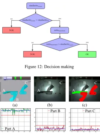
The workflow of the decision-making step is shown in
Fig.12. The decision is taken using two indicators: the
sim-ilarity score (simsim-ilarityscore) based on Shape Context and
the matched ratio (matchedratio) represented by the ratio
be-tween matched and not matched edgelets.
In Fig. 13, we show the CAD model, the RGB image
acquired by the inspection camera, and the final result on two different cases (element OK and element NOK).
Version October 14, 2019 submitted to J. Imaging 14 of 28 100 200 300 400 500 600 700 X Axis 100 200 300 400 500 600 700 800 900 Y Axis
All projected edgelets Matched edges Matched filtered edgelets
Figure 15.The shapes used in the Shape Context approach
The workflow of the making decision step is shown in Fig.16The decision is taken using two
313
indicators: the similarity score (similarityscore) and the matched ratio (matchedratio) represented by the
314
relationship between matched and not matched edgelets.
315
similarityscore> similarityth similarityscore
ratiomatched
ratiomatched> similarityscore NOK NOK OK no yes yes no 1 Figure 16.Decision making
In Fig.17, we show the matchedratioand matchedthcomputed on two different cases (element
316
OK and element NOK).
317
• If similarityscore< similarityth, the element is considered NOK (absent or incorrectly mounted).
318
In our experiments we have set similarityth= 0.7, based on an extensive comparison between
319
different shapes.
320
• If similarityscore> similarityth, we compute the ratio between the number of matched edgelets
321
and the number of not matched edgelets (matchedratio).
322
Figure 12: Decision making
A B C A B C A B C (a) (b) (c) 0 20 40 60 80 100 0 20 40 60 80 Part A 0 20 40 60 80 100 0 20 40 60 80 Part B 0 20 40 60 80 0 20 40 60 80 Part C
Figure 13: (1st row) (a) CAD model, (b) 2D inspection
image, and (c) result of inspection with green OK (ele-ment present) and red NOK (ele(ele-ment absent or incorrectly
mounted), (2nd row) respectively the matched
ratio (curve)
and threshold matchedth (red horizontal line) computed on
the three different cases 100 times: element A (present) in green, element B (incorrectly mounted) in red, and element C (absent) in red
3.6. Metrics used for evaluation 3.6.1. Accuracy, sensitivity, specificity
Table 1 outlines definitions of the true positive (TP), the
false positive (FP), the true negative (TN) and the false neg-ative (FN) in defect detection.
Table 1: Definitions of TP, FP, TN, FN in defect detection Actually defective Actually non-defective Detected as defective TP FP Detected as non-defective FN TN
Based on these notations, the detection success rate (known also as detection accuracy) is defined as the ratio of correct assessments and number of all assessments. Sensitivity is defined as the correct detection of defective samples. Sim-ilarly, the specificity can be defined as the correct detection of defect-free samples. Finally, the overall accuracy could
be calculated based on the metrics of sensitivity and speci-ficity. The accuracy, sensitivity and specificity are defined as: accuracy = TP + TN TP + FN + TN + FP sensitivity = TP TP + FN specificity = TN TN + FP 3.6.2. Precision and Recall
Precision and recall metrics are used to validate the perfor-mance of defect detection. Precision and Recall are defined as: precision = TP TP + FP recall = TP TP + FN Fscore= 2 × precision × recall precision + recall
The Fscoreis calculated to measure the overall performance
of a defect detection method. The highest value of the Fscore
is 100% while the lowest value is 0%. 3.7. Evaluation
The approach was tested on a dataset acquired in a factory with a total number of 43 inspected elements and 643 im-ages. Elements are inspected one by one and decision on each of them is based on one acquired image. The distance between camera and inspected element has been set at 600 mm with a tolerance of ±6mm. Some examples of our
dataset used to evaluate our approach are shown in Fig.14.
It can be noted that our dataset is acquired in a context of in-dustrial robotized inspection in conditions of very cluttered environment.
The overall performance of our method is represented by Fscore = 91.61%. The values of specificity, accuracy,
sensitivity, precision and recall of our method are shown in
Tables2and3.
Table 2: Result of the evaluation (TP, TN, FP, and FN) Nbr of
elements
Nbr of
images TP TN FP FN
43 643 344 236 63 0
The experimental results show that our proposed ap-proach is promising for industrial deployment.
The main challenge we faced lies in the fact that our dataset is acquired in a factory, on a real and very com-plex assembly at the very end of the production line (almost all the elements are mounted). Therefore, the environment
Figure 14: Some examples of our dataset used to evaluate our approach in a context of robotized inspection in
condi-tions of very cluttered environment: (1stand 3rdrows) real
images, (2ndand 4throws) corresponding renders of CAD
models
Table 3: Performance measures
Accuracy Sensitivity Specificity Precision Fscore
90.20% 100% 78.93% 84.52% 91.6%
around inspected element is very cluttered and the matching task becomes more difficult.
Please refer to our recent paper [1] for more detailed
ex-planation of the experiments and especially the comparison of the evaluation of the hand-held tablet inspection system and the robotic inspection platform.
4. Inspection by 3D point cloud analysis
The strategy based on 3D point cloud data is used when 2D image processing is not sufficient. Indeed, sometimes, using 3D data is necessary, for example for checking if the distance between two cables is conform to the security stan-dards. These types of defects are undetectable with an RGB camera because the cables have the same color. Moreover, obtaining distance measurements is challenging in the ab-sence of depth information.
More precisely, it is required to check if two flexible
elements (e.g. cables, harnesses) or a flexible and a rigid element (e.g. pipe, support) are at a safe distance from each
other. Fig.15illustrates that 2D image analysis is not
suffi-cient to solve this type of inspection problem.
CAD image
2D image
Figure 15: Example of 3D inspection: (left) airplane en-gine (right) the interference between some cables cannot be determined by 2D image analysis
The online inspection process consists of several steps, which are detailed in this section: (1) a 3D point cloud is acquired using the pre-calibrated Ensenso N35 3D scanner
mounted on the robot arm (Fig. 16), (2) a two-step
global-to-local registration procedure that allows for alignment of the 3D data with the 3D CAD model is performed, (3) the cables are segmented from the 3D point cloud, (4) the dis-tance between each cable and its surrounding environment is computed in order to detect a possible interference prob-lem, (5) the bending radius of each cable is computed.
Figure 16: Pre-calibrated Ensenso N35 3D scanner
4.1. 3D cable segmentation
Cables are designed to be flexible. The registration or
matching with 3D CAD model becomes problematic when the target objects are non-rigid, or prone to change in shape
or appearance. Nevertheless, cable connection points,
where the cable meets connectors or clamp, are rigid. These connection points are the most important elements for aligning with CAD model. Indeed, these points make it possible to guarantee a rigidity of a portion of cable.
After some preprocessing steps such as known noise removal techniques as well as subsampling CAD model mesh, we proceed to a global 3D/2D alignment phase. The results of the global registration are refined by a local reg-istration process that uses an iterative non-linear ICP
pro-posed by Besl and McKay [8] and Levenberg-Marquardt
We further perform segmentation of a cable by model-ing it as a set of cylinders. We propose a search structure that allows to find the cables present in the real point cloud and to reconstruct them as collections of cylinders of vary-ing radius, length, and orientation. Each cylinder, called sub-cable is fitted, using the point-to-point ICP algorithm
[10], to the point cloud data corresponding to a cable. More
details about our method can be found in our recent papers [2] [3].
The final result of the cable segmentation phase can be
seen in Fig.17.
(a) (b)
Figure 17: (a) the final cylinder model (made of 12 sub-cables) in green and, in blue, a detected hole in the cable due to two overlapping cables (1 sub-cable) and (b) the seg-mented point cloud
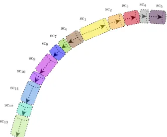
Fig. 18and Table4illustrate the final cylinder model
shown in Fig. 17made of 13 consecutive sub-cables
la-beled sc1through sc13. Fig.18shows the details of the 13
sub-cables: their radius, the length, the angle between two consecutive main axis and the direction of the propagation, where ‘+’ denotes first direction and ‘-’ denotes second
di-rection. The angle between two consecutive main axis θi
can easily be computed by considering each main axis to be a vector and by taking the dot product of the two vec-tors:
v1· v2= |v1||v2| · cos(θi) (1)
4.2. Interference detection and bend radius computa-tion
The global objective of the inspection process is to measure (1) the minimum distance between each segmented cable and the other elements in the mechanical assembly (in order to check a possible interference problem), and (2) the bend radius of each segmented cable (in order to check that it complies with safety standards).
4.2.1. Inputs
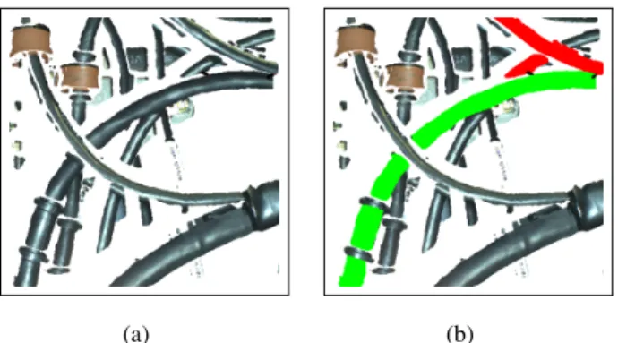
After the segmentation process, we have two main point
clouds: the segmented point cloud, which we will call Ps,
and all the other points, excluding the segmented point
cloud, which we will call Ps(see Fig. 19). If we call P
sc5 sc4 sc3 sc2 sc1 sc6 sc7 sc8 sc9 sc10 sc11 sc12 sc13
Figure 18: An illustration of the final cylinder model shown
in Fig. 17made of 13 consecutive sub-cables labeled sc1
through sc13(different colors denote the sub-cable models)
Table 4: The details of the 13 sub-cables: their radius, the length, the angle between consecutive main axis and the direction of propagation, where ‘+’ denotes first direction and ‘-’ denotes second direction. It should be noted that
sc8 is a detected hole due to the overlapping cables (see
Fig. 17) and its radius is equal to the radius of previous
sub-cable sc7
Sub-cable Radius length Angle Direction
sc1 5.81 33.55 – + sc2 5.93 22.09 8.51 + sc3 5.89 17.83 2.12 + sc4 5.97 17.97 11.4 + sc5 5.91 19.26 3.7 + sc6 5.90 16.43 4.12 -sc7 5.91 10.01 2.02 -sc8 – 13.20 3.22 -sc9 5.93 22.01 1.7 -sc10 5.98 10.66 1.1 -sc11 5.92 19.44 4.3 -sc12 5.79 11.81 12.3 -sc13 5.80 18.02 11.2
-the filtered input 3D point cloud provided by -the 3D
scan-ner, we have P = Ps+ Ps.
4.2.2. Interference detection
In this section we will focus on the detection of a possi-ble interference between a capossi-ble and the other surrounding elements (another cable, a support, etc.) present in the me-chanical assembly.
The objective is to determine if the cables are at a safe
distance dT from the other surrounding elements present
5.3.2 Interference detection
In this section we will focus on the detection of a possible interference between a cable and the other surrounding elements (another cable, a support, etc.) present in the mechanical assembly.
Inputs: After the segmentation process, we have two main point clouds: the segmented point cloud, which we will call Ps, and all the other points, excluding the segmented point cloud, which
we will call Ps(see Fig.33). If we call P the filtered input 3D point cloud provided by the 3D
scanner, we have P = Ps+Ps.
Zoom
Fig 33: The segmented point cloud, which we will call Psin green and all the other points,
exclud-ing the segmented point cloud, which we will call Psin red
All input data are presented in Table3.
Table 3: Inputs
Name Role
P Filtered input real point cloud Ps Segmented point cloud (a cable)
Ps
All filtered input points, excluding the segmented point cloud dT Tolerance (interference distance)
39
Figure 19: The segmented point cloud, which we will call
Psin green and all the other points, which we will call Ps
in red
detection process is shown in Fig.20.
(a) (b)
Figure 20: Result of interference detection process: (a) the input point cloud, (b) segmented point cloud in green and representative clusters which cause interference problem in red
Our experiments have been detailed extensively in our
recent paper [3].
For one of the experiments we use the available CAD model. We identified 4 cables and measured the distance between each cable and its surrounding elements in the as-sembly. We do this with a specialised modelling software
CATIA©. Further, we sampled the cables and the elements
and added noise to the sampled point cloud. This step sim-ulates the noise introduced by the process of scanning. We added three different levels of noise. Finally, we run our algorithm on all generated clouds and obtain the minimal distance between each segmented cable and the other ele-ments. We compare this result with the measure obtained
with CATIA©. Table5shows that the obtained results are
satisfactory.
4.2.3. Bend radius calculation
The other objective of the inspection process is to measure the bend radius of each segmented cable (in order to check that it complies with safety standards).
The minimum bend radius is the smallest allowed ra-dius the cable is allowed to be bent around. The 3D
seg-mentation method presented in section4.1produces almost
immediately a cable model segmented from the
measure-ment data (see Fig. 21a). Using this model, we can carry
Table 5: Interference measurement results compared with
the CATIA©modelling software
Standard deviation of added noise Measure obtained with CATIA Measure obtained by our algorithm 0 13.5 13.34 0.4 15.5 14.63 0.8 14 12.23 1.2 18.5 16.38
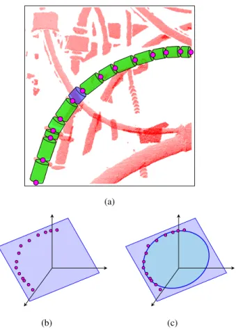
out a quantitative analysis of the bend radius of the cable. In order to estimate the bend radius of a cable, we fit
a 3D plane to the set of start-points Pskand end-points Pek
for all the estimated sub-cables sck(see Fig.21a). Further
we project all the points onto the fitted plane (see Fig.21b).
Finally, the bend radius is estimated by fitting a circle to
the set of projected 2D points (see Fig.21c). Therefore, the
accuracy of the measure is directly related to the robustness of the segmentation algorithm, fitting plane algorithm and fitting circle algorithm.
Since we do not have the needed instrumentation to measure precisely the bend radius of the cables within the mechanical assembly, we have decided to test our approach on synthetic data generated from the CAD model. A few
examples of our dataset are shown in Fig.22.
The minimum allowed bend radius is based on the di-ameter and the type of cable. By industry standards, the rec-ommended bend radius for harnesses should not be lower than 10 times the diameter of the largest cable.
The results are evaluated on the basis of the difference
between the ground truth bend radius Rcand the estimated
bend radius eRc: M SEbend radius= 1 n n X i=1 (Rci− eRci) 2 (2)
On a set of 3 different cables with different, radius,
res-olutions and different bend radius, we found M SEbend radius
= 1.23 mm.
As expected, we have found that the results are better when the number of sub-cables found is high. Indeed, the fitting of plane or circle are more accurate when the set of
start-points Psand end-points Pecontains more points.
5. Conclusion
We proposed an automated inspection system for mechan-ical assemblies in an aeronautmechan-ical context. We address the problem of inspection in two parts: first, automatic selec-tion of informative viewpoints before the inspecselec-tion pro-cess is started, and, second, automatic treatment of the ac-quired images and 3D point clouds from said viewpoints by matching them with information in the 3D CAD model.
(a)
(b) (c)
Figure 21: Steps for calculating the bend radius: (a)
segmentation modeling result, where each sub-cable sck
(green) has an initial point Pk
s and a final point Pek(both in
pink), (b) projection of all the points Psand Peonto the 3D
plane previously obtained by fitting a plane to those same points with a least squares method, and (c) fitting a circle by least squares method to these projected 2D points
Rc= 13.65 cm (a) Rc= 14 cm (b) Rc= 46.55 cm (c) Fig 48: A few examples of our dataset. Three different synthetic cables with different bend radius (Rc)
The results are evaluated on the basis of the difference between the ground truth bend radius Rcand the estimated bend radius eRc:
M SEb. radius= 1 n n X i=1 (Rci− eRci) 2 (11)
In order to estimate the bend radius of a cable, we fit a 3D plane to the set of start-points Ps and end-points Pefor all the estimated sub-cables. Further we project all the points onto the fitted plane. Finally, the bend radius is estimated by fitting a circle to the set of projected 2D points. Therefore, the accuracy of the measure is directly related to the robustness of the segmentation algorithm, fitting plane algorithm and fitting circle algorithm.
On a set of 3 different cables with different, radius, resolutions and different bend radius, we found M SEb. radius= 1.23 mm.
As expected, in our experience we have found that the results are better when the number of sub-cables found is high. Indeed, the fitting of plane or circle are more accurate when the set of start-points Psand end-points Pecontains more points.
57
Figure 22: A few examples of our dataset. Three different
synthetic cables with different bend radius (Rc)
Depending on the inspection type and speed/accuracy trade off, we propose two strategies: the first one is based on 2D image analysis and the second one relies on 3D point cloud analysis.
With our 2D strategy we are focusing on detecting miss-ing and badly mounted rigid parts by comparmiss-ing sensed in-formation with the CAD model.
In the second part of the paper we give an overview of our 3D based method for cable segmentation based on cylinder fitting. Using the segmentation result and the CAD model, we can carry out quantitative analysis of potential interferences and the computation of the bend radius of each cable.
The experimental results show that our method is highly accurate in detecting defects on rigid parts of the assembly as well as on aircraft’s Electrical Wiring Interconnection System (EWIS).
Acknowledgements
This research work has been carried out within a PhD thesis co-funded by the French ”R´egion Occitanie”. We would like to thank the R´egion Occitanie for its financial support.
References
[1] H. Ben Abdallah, I. Jovancevic, J.-J. Orteu, L.
Br`ethes. Automatic inspection of aeronautical me-chanical assemblies by matching the 3D CAD model and real 2D images. Journal of Imaging, 8(10):81-110, October 2019.
[2] H. Ben Abdallah, J.-J. Orteu, B. Dolives, I.
Jovance-vic. 3D Point Cloud Analysis for Automatic Inspec-tion of Aeronautical Mechanical Assemblies. 14th In-ternational Conference on Quality Control by Artifi-cial Vision (QCAV), Mulhouse, France, May 2019.
[3] H. Ben Abdallah, J.-J. Orteu, I. Jovancevic, B.
Do-lives. 3D Point Cloud Analysis for Automatic In-spection of Complex Aeronautical Mechanical As-semblies. Journal of Electronic Imaging (submitted in 2019).
[4] A. Loesch, S. Bourgeois, V. Gay-Bellile, M. Dhome.
Generic edgelet-based tracking of 3D objects in real-time. International Conference on Intelligent Robots Systems (IROS), pp. 6059-6066, 2015.
[5] S. Xie, Z. Tu, Holistically-Nested Edge Detection.
IEEE International Conference on Computer Vision (ICCV), 2015.
[6] J. Canny, A Computational Approach to Edge
Detec-tor. IEEE Transactions on PAMI, pp. 679-698, 1986.
[7] S. Belongie, J. Malik, J. Puzicha. Shape matching;
ob-ject recognition using shape contexts. IEEE Transac-tions on Pattern Analysis; Machine Intelligence, 24, pp. 509-522, 2002.
[8] P.J. Besl, N.D. McKay. A method for registration of
3-D shapes. IEEE Transactions on Pattern Analysis and Machine Intelligence, pp. 239-256, 1992.
[9] C. Kim, H. Son, C. Kim. Fully automated registration
of 3D data to a 3D CAD model for project progress monitoring. Image and Vision Computing, pp. 587-594, 2013.
[10] S. Rusinkiewicz, M. Levoy. Efficient variants of the ICP algorithm. Proceedings of Third International Conference on 3-D Digital Imaging and Modeling, pp. 145-152, 2001.