Diagnostic de la variabilité interne d'un ensemble de simulations du Modèle Régional Canadien du Climat

UNIVERSITÉ DU QUÉBEC

À

MONTRÉAL

DIAGNOSTIC DE LA VARIABILITÉ INTERNE D'UN ENSEMBLE DE

STh1ULATIONS DU MODÈLE RÉGIONAL CANADIEN DU CLIMAT

MÉMOIRE

PRÉSENTÉ

COMME EXIGENCE PARTIELLE

DE LA MAÎTRISE EN SCIENCES DE L'ATMOSPHÈRE

PAR

OUMAROU NIKIEMA

UNIVERSITÉ DU QUÉBEC

À

MONTRÉAL Service des bibliothèques

Avertissement

La diffusion de ce mémoire se fait dans le respect des droits de son auteur, qui a signé le formulaire Autorisation de reproduire et de diffuser un travail de recherche de cycles supérieurs (SDU-522 - Rév.ü1-2üü6). Cette autorisation stipule que «conformément

à

l'article 11 du Règlement no 8 des études de cycles supérieurs, [l'auteur] concède

à

l'Université du Québec

à

Montréal une licence non exclusive d'utilisation et de publication de la totalité ou d'une partie importante de [son] travail de recherche pour des fins pédagogiques et non commerciales. Plus précisément, [l'auteur] autorise l'Université du Québec

à

Montréal

à

reproduire, diffuser, prêter, distribuer ou vendre des copies de [son] travail de recherche

à

des fins non commerciales sur quelque support que ce soit, y compris l'Internet. Cette licence et cette autorisation n'entraînent pas une renonciation de [la] part [de l'auteur]

à

[ses] droits moraux ni

à

[ses] droits de propriété intellectuelle. Sauf entente contraire, [l'auteur] conserve la liberté de diffuser et de commercialiser ou non ce travail dont [il] possède un exemplaire.»

REMERCIEMENTS

La rédaction de ce mémoire a été rendue possible grâce au soutien continuel

de mon directeur de recherche, Monsieur René LAPRISE membre du Réseau

Canadien en Modélisation et Diagnostics du Climat Régional. Je vous remercie

Monsieur le Professeur pour m'avoir appuyé et donné l'opportunité de réaliser ce

projet.

J'adresse un vif remerciement aux évaluateurs de ce mémoire, ainsi qu'à

l'ensemble du corps professoral pour son immense appui. Mention spéciale

à

mes

collègues et toute l'Équipe de Simulations Climatiques d'Ouranos, que je remercie.

Je ne saurais terminer sans mentionner mon épouse Hawa SA WADOGO et ma

fille Sarah NIKIEMA pour leur soutien, sans oublier Ismael NIKIEMA pour ces

sourires intermittents!!!!

TABLE DE MATIÈRES

LISTE DES FIGURES v

LISTE DES ABREVIATIONS, SIGLES ET ACRONYMES vii

LISTE DES SYMBOLES viii

RÉSUMÉ xi ABSTRACT xii INTRODUCTION 1 CHAPITRE 1 5 Abstract 7 1. Introduction 8

2. Equations for the time-evolution of the Internai Variability 10

2.1. The potential temperature IV equation 11

2.2. The relative vorticity IV equation 16

2.3. Domain, Simulation and Evaluation methods 19

3. Results and Analysis 21

3.1. Vertical profile and time evolution of the IV 21

3.2. Validation of the Internai Variability budget equation 24

3.3. Spatial patterns of the internai variability tendency 24

3.4. Time evolution of the domain-average internai variability tendency 25

IV

3.4.2. Budget of the relative vorticity IV 28

4. Conclusions 30

FIGURES 34

CONCLUSION 49

APPENDICES 54

LISTE DES FIGURES

Figure Page

1

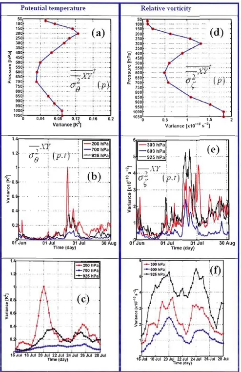
(a, d) Vertical profile of time- and domain-averaged inter-member variance for the potential temperature and the relative vorticity. The 1050-hPa level is an extrapolation of the 1000-hPa level ; (b, c, e, f) time evolution of the domain average valiance for the potential temperature and relative vorticity at different pressure levels . 35

2 Time-averaged over 3-month period of the inter-member variance for

the potential temperature (a, b, c) and the relative vorticity (d, e, f).

The domain of interest is shown in Fig. 2a .. 36

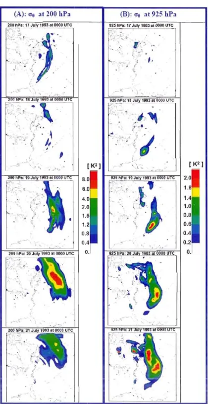
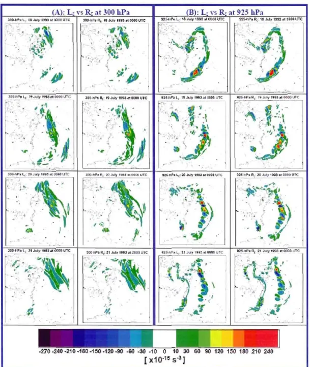
Field of inter-member variance for the potential temperature at (A) 200 hPa and (B) 925 hPa, during the period of large increase of IV

from 17 to 21 luly (see Fig. le) . 37

3

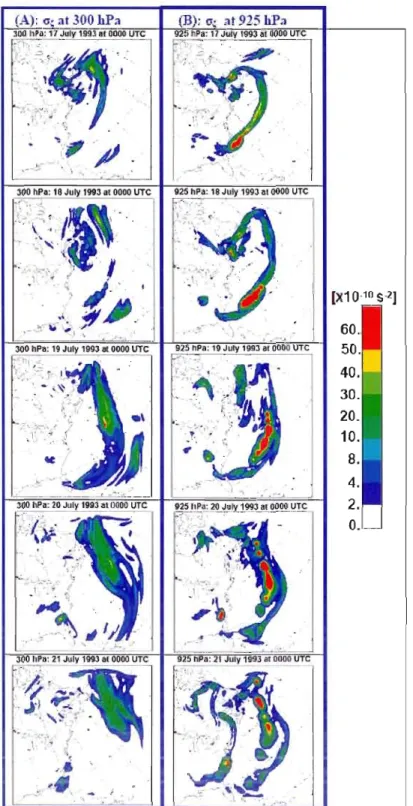
4 Field of inter-member variance for the relative vorticity at (A) 300 hPa and (B) 925 hPa, during the period of the large increase of IV from 17

to 21 luly (see Fig. lf) .. 38

5

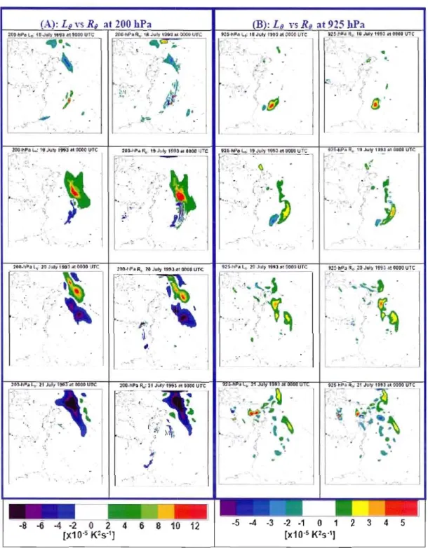
Left-hand side term (Lo) and the sum of ail right-hand side terms (Ra)

of the potential temperature inter-member variance equation on celtain dates of the period of interest at different pressure levels: (A) 200 hPa

and (B) 925 hPa . 39

Left-hand term (Lç) and the sum of ail light-hand terms (Rç) of the relative vorticity inter-member variance equation du ring the peliod of interest at different pressure levels: (A) 300 hPa, (B) 925 hPa ..

40

6

7 Dispersion diagram of ail grid points (except the sponge zone) to

illustrate the comparison between the left-hand tenn and the sum of ail right-hand terms at different pressure levels for the (A) potential

VI

8

Time evolution of the left-hand tenn and the sum of ail right-hand terms of the domain-averaged inter-member variance equations for the potential temperature (a, c) and the relative vorticity (b, d) at different pressure levels; (e, f) dispersion diagram to illustrate the comparison

between these two sides of the equation . 42

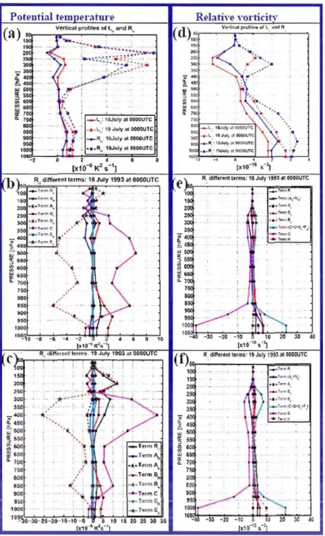
9

Vertical profiles of R different telms of the domain-averaged inter­ member variance equation for the potential temperature (a, b, c) and the relative vorticity (d, e, f). The 1050-hPa level is an extrapolation of

the 1000-hPa level. . 43

10 Time evolution of different tenns on the right-hand side of domain­ averaged inter-member variance equations for the potential temperature (a, b) and the relative vorticity (c, d, e, f) during the

period of interest. . 44

11 Field of each term on the right-hand side of the inter-member variance equation for the potential temperature on 20 July 1993 at 0000

urc

at different pressure levels: (A) 200 hPa and (B) 925 hPa ... 45

12 Fields of each tenn on the right-hand side of the inter-member variance equation for the relative vorticity on 20 July 1993 at 0000 UTC at different pressure levels: (A) 300 hPa, (B) 925 hPa . 46

13 Time evolution of different parts in terms BI' (a, b) and C (ef) of the potential temperature IV equation. Different fields show the covariance of fluctuations in BI' at (c) 400 hPa and (d) 850 hPa, and the covariance of fl uctuation associated to (g) condensation (precipitation) and (h) convection in C at 400 hPa. Fields are valid on

July, 19 at 0000 UTC. . 47

14 Time evolution of the covariance of fluctuation in

Bh

of the (A) potential temperature IV equation and the (B) relative vorticity IV equation. Different fields show the covariance of fluctuations in Bh at

LISTE DES ABREVIATIONS, SIGLES ET

CI CRCM GCM IC

IV

LBC MCG MRC MRCC NCEP RCM SST UQAM US VI

ACRONYMES

Conditions initiales

Canadian Regional Climate Model

General Circulation Model

Initial Conditions

Internai Variability

Lateral Boundary Conditions

Modèle de Circulation Générale

Modèle Régional de Climat

Modèle Régional Canadien du Climat

National Centers for Environmental Prediction

Regional Climate Model

Sea SUlface Temperature

Université du Québec à Montréal

United States

LISTE DES SYMBOLES

c constante de diffusion horizontale

Cp coefficient de chaleur spécifique à pression constante

f

paramètre de Coriolis

F, sources et puits de la quantité de mouvement pour la composante U du vent

Fy sources et puits de la quantité de mouvement pour la composante V du

vent

indice de points de gJilie dans la direction X

nombre total de point de grille dans la direction X

j indice de points de grille dans la direction Y ] nombre total de point de grille dans la direction Y

ln sources et puits de la température potentielle pour le membre

n

k indice de points de grille dans la direction Z

Le

tendance de la Vlpour la température potentielle

L( tendance de la V 1 pour le tourbillon relatif

LIfJ tendance de la V 1 pour une variable quelconque <p

m facteur d'échelle pour une projection stéréographique polai re

n numéro du membre

N nombre total de membre

P pression

Po pression de reference

R

constante des gaz pour l'air sec

Re

somme de tous les termes de droit de l'équation de la VI pour la température potentielle

ix

relatif

Rif!

S

somme de tous les termes de droite de l'équation de la VI pour une

variable quelconque q> tenne de projection T LI Un temps Température

composante du vent horizontal réel selon x

composante du vent horizontal modèle dans la direction X pour le

membre n v

Vn

composante du vent horizontal réel selon y

composante du vent horizontal modèle dans la direction Y pour le

membre n w

x

composante de la vitesse verticale selon z

coordonnée du référentiel cartésien local dans la direction est

X

y

y

z

nI

coordonnée de la projection stéréographique polaire

coordonnée du référentiel cartésien local dans la direction nord

coordonnée de la projection stéréographique polaire

coordonnée du référentiel cartésien local dans la direction verticale

opérateur de la moyenne temporelle

n

XY

opérateur de la moyenne spatiale sur un domaine d'intérêt

( ) opérateur de la moyenne d'ensemble

5

ç

opérateur différentiel tourbillon relatif () K

A

CT,

température potentielle

coefficient de chaleur spécifique à pression constante (R/Cp )

longitude

x (je qJ

r

rjJ

'II

variance ou VI pour la température potentielle

variable atmosphérique quelconque

nombre total d'archivage

hauteur du geopotentiel

lati tude

'110

latitude de référence

"

"

RESUME

Les Modèles Régionaux du Climat (MRC) ont longtemps été considérés comme

des outils performants, de haute résolution

à

aire limitée permettant une meilleure

compréhension du climat passé, présent et futur. Le plus souvent, les MRC sont

pilotés

à

leurs frontières latérales par des Modèles Globaux du Climat (MGC) de

basse résolution, et qui couvrent le reste du globe terrestre. Ces modèles ont la

particularité de reproduire différentes solutions de l'état de l'atmosphère

à

cause de

leur sensibilité aux conditions initiales (CI). Outre la solution due aux forçages

externes (forçage aux frontières latérales et le forçage de surface), les MRC

reproduisent une seconde solution associée

à

la variabilité interne (VI) du modèle du

fait de leur sensibilité aux CI. Cette sensibilité est en grande partie causée par la

nature non-linéaire de la physique et la dynamique atmosphériques.

À

l'instar de précédentes études, nous analysons la variabilité interne du Modèle

Régional Canadien du Climat (MRCC) en utilisant un ensemble de simulations aux

CI différentes. Ce projet de recherche consiste

à

effectuer un diagnostic quantitatif

des termes dynamique et diabatique qui contribuent à la variation temporelle et la

distribution spatiale de la VI. L'originalité de ce travail est qu'il propose des

équations bilans de la VI pour deux variables atmosphériques: la température

potentielle et le tourbillon relatif. Les deux équations établies présentent des termes

similaires, notamment les termes relatifs au transport de la VI par l'écoulement de la

moyenne d'ensemble et la covariance des fluctuations agissant sur le gradient de la

moyenne d'ensemble de la variable considérée.

Concrètement, nous avons utilisé un ensemble de 20 simulations aux CI

différentes pour analyser les caractéristiques de la VI, afin de déterminer une période

et une région d'intérêt caractérisées par une forte croissance de la VI. Ensuite, nous

avons validé les équations établies en montrant l'égalité entre les deux parties de

chaque équation. Enfin, une étude de bilan a permis d'évaluer la contribution des

différents termes au développement et

à

l'évolution de la VI. Les résultats révèlent

que les termes dominants responsables de l'accroissement de la VI sont soit les

termes de covariance impliquant les fluctuations de température potentielle et de

chauffage diabatique, ou les termes de covariance de fluctuations inter-membres

agissent sur le gradient de la moyenne d'ensemble de la variable considérée. Les

résultats révèlent également que les épisodes de fortes diminutions de la VI se

produisent lorsque les maxima de la VI sont proches de la frontière nord-est,

indiquant leur transport en dehors de la zone d'étude par l'écoulement moyen. Enfin,

nos résultats ont montré qu'en moyenne, les termes du troisième ordre sont

négligeables, mais peuvent devenir importants lorsque la VI est importante.

Mots

clés: Équation de la variabilité interne, modèle régional de climat, ensemble de

simulations, climat de l'Amérique du Nord.

ABSTRACT

The regional climate models (RCM) have long been considered as powerful tools that allow better understanding of climate, because of their high resolution on limited areas. Most often, the RCM are driven at theirs lateral boundaries by a low resolution model (Global Climate Models, GCM), which covers the entire earth. These models have a particularity to reproduce different solutions of the atmospheric state due to their sensitivity to initial conditions (IC). Besides the solution resulting from externat forcing, the MRC reproduce other solution associated with internai variability (IV) due to their sensitivity to le. This sensitivity is caused by the chaotic and nonlinear nature of the atmospheric dynamics.

As in like previous studies, we analyze the Canadian RCM internai variability using an ensemble of simulations run with different le. This project performs a quantitative diagnostic of dynamic and diabatic terms that contribute to the temporal variation of IV. The originality of this work is that it proposes budget equations of the IV of two atmosphelic variables: potential temperature and relative vorticity. For both of these variables, the IV equations present similar terrns, notably terms relating to the transport of IV by ensemble-mean flow and to the covariance of fluctuations acting on the gradient of the ensemble-mean state.

In practice, we used a set of 20-member set of simulations that differ only in their IC to analyze the IV characteristics. We identify a period and an area of interest characterized by large IV variations. Then, we show the skill of these equations to diagnose the IV by comparing both si des of each equation. Finally, we assess the quantitative contribution of each term to the IV tendency. Our study suggests that the dominant terms responsible for the large increase of IV are either the covariance term invoJving the potential temperature fluctuations and diabatic heating fluctuations, or the covariance of inter-member fluctuations acting upon ensemble-mean gradients. Results also reveal that the episodes of large decreases of IV occur when the maximum of IV are close to the northeast boundary, and eventually get transported out of the regional domain by the ensembJe-mean flo\\'. Finally, our results reveal that, on average, the third-order terms are negligible, but they can become important when the IV is large.

Keywords: internai variability equation, - Regional climate models - Ensemble of simulations - North American climat

INTRODUCTION

L'atmosphère est constituée d'un fluide qui obéit aux principes fondamentaux de

la mécanique des fluides et de la thermodynamique. Elle est caractérisée par plusieurs

paramètres tels que la température, la pression, l'humidité, la teneur en eau liquide et

la vitesse (horizontale et verticale) de l'air. L'évolution de tous ces paramètres peut

être suivie en utilisant leur équation d'évolution respective. Ainsi, les prévisions

climatiques à court, moyen et long terme sont faites grâce aux modèles numériques basés sur certaines lois de la physique, notamment les lois thermodynamiques, de

conservation de la masse et les équations d'Euler qui décrivent l'évolution d'un fluide

à la surface d'une sphère en rotation.

De nos jours, à cause de leurs performances et de leurs capacités à reproduire les processus physiques de l'atmosphère avec une haute résolution, les Modèles

Régionaux du Climat (MRC) sont utilisés pour simuler le climat passé, présent et

futur. Les MRC sont intégrés sur un domaine à aire limitée avec des conditions

initiales (Cf) et des conditions frontières latérales (CFL) fournies par un modèle de

circulation générale (MCG) ou par des données de ré-analyses. Le pilotage

unidirectionnel du MCG vers le MRC consiste en une transmission d'informations de

la grande échelle vers la petite échelle, rendant ainsi possible le calcul à haute résolution.

À l'instar des modèles de circulations générales, les MRC sont sensibles aux CI

en raison du caractère non-linéaire de la dynamique atmosphérique (Lorenz 1963);

cependant les CFL exercent une contrainte qui limite le degré de liberté des modèles

pilotés. Il est maintenant démontré que les MRC développent un certain degré de

variabilité interne (VI. défini comme étant la différence qui existe entre les

simulations exécutées avec différentes Cl) en raison des non-linéarités de la physique

et de la dynamique du modèle (Weisse et al. 2000; Giorgi et Bi 2000; Rinke et

Dethloff 2000, Christensen et al. 2001; Caya et Biner 2004; Rinke et al 2004;

2

Dans leurs simulations réalisées sur un domaine couvrant l'est de l'Asie, Giorgi et

Bi (2000) ont montré que la VI du modèle est maximale en été et très faible en hiver.

La forte VI en été serait liée aux non-linéarités associées aux processus de convection

et de précipitations, alors qu'en hiver, le fort courant jet d'ouest réduit la variabilité du

modèle en raison des intenses forçages exercés aux frontières latérales. Un important

résultat de leur étude est que la VI semble être liée aux régimes saisonniers et

synoptiques.

Dans leur étude sur un domaine de j'Arctique, Rinke et Dethloff (2000) et Rinke

et al. (2004) ont montré que le contrôle exercé par les CFL est plus faible comparé

aux domaines de moyenne latitude. Ils ont constaté que la VI est importante en

automne/hiver, et faible en été. Ce résultat est une conséquence de la circulation

particulière de l'Arctique et de l'activité des ondes planétaires qui sont faibles en été.

Christensen et al. (2001) ont porté une attention à la variabilité interne en comparant les simulations de deux MRC réalisées sur une même zone

méditerranéenne. Ils ont constaté que la VI du modèle dépend du type de variable

étudié, des caractéristiques du modèle, ainsi que de la zone d'intégration. Toutefois,

les intensités de la variabilité sont d'un ordre de grandeur comparable pour les deux

modèles. Leur étude a également montré l'impact de la VI sur la précision des

résultats du MRC.

Caya et Biner (2004) ont étudié la VI dans les simulations du Modèle Régional

Canadien du Climat (MRCC) sur un domaine couvrant l'est de l'Amérique du Nord et

une partie de l'océan Atlantique. Comme Giorgi et Bi (2000), ils ont trouvé de faibles

intensités de la VI en hiver, au printemps et en automne, et de forte intensité en été,

de sorte que les simulations seraient palfois différentes pour les mêmes situations

météorologiques. Lucas-Picher et al. (2004, 2008) ont constaté que, pour une saison

donnée, l'ordre de grandeur de la VI est directement lié à la taille du domaine.

Contrairement aux études précédentes, ils ont constaté une importante VI en hiver

3

Récemment, Alexandru et al. (2007) ont étendu les études antérieures avec le

MRCC sur le domaine de l'Amérique du Nord en utilisant un ensemble de 20

simulations réalisées pour la saison de l'été 1993. Leurs résultats montrent que durant

l'intégration l'intensité de la VI varie fortement avec les événements synoptiques. La

répartition géographique de la VI dépend des variables étudiées. Les fortes

précipitations dans le sud des États-Unis semblent agir comme un mécanisme

déclencheur de la VI pour la hauteur du géopotentiel à 850 hPa. Celle-ci se développe

le long des trajectoires des tempêtes et elle atteint son maximum dans la partie nord­

est de la région d'étude.

Les travaux antérieurs ont mis en évidence la présence de VI dans les simulations

des MRC, toutefois leur intensité est faible comparée à celle des modèles de

circulations globales à cause du contrôle exercé aux frontières latérales. Les

mécanismes physiques responsables du développement épisodique de la VI semblent

être difficile à élucider. Certaines hypothèses ont été émises sur ces mécanismes qui favorisent le déclenchement de forte VI, notamment les non-linéarités associées à la

transmission d'information de la grande échelle vers les petites échelles, les non­

linéarités associées aux processus de paramétrisation diabatique telle que la

condensation et la convection, les instabilités hydrodynamiques associées aux forts

gradient de température et du vent. Ce projet vise à approfondir notre compréhension

du processus de développement de la VI en effectuant un diagnostic quantitatif des

différentes contributions à la variation temporelle et la distribution spatiale de la VI.

Dans la section 2 de l'article de ce mémoire, nous présentons la méthodologie utilisée

pour établir les équations bilans de la VI pour la température potentielle et le

tourbillon relatif. Dans la section 3, nous présentons les différents résultats obtenus en

utilisant une base de données issue des travaux d'Alexandru et al. (2007). Nous

commençons par étudier les caractéristiques de la VI de l'ensemble des simulations

réalisées avec différentes CI. Ensuite, nous étudions la validité de ces équations en

vérifiant l'égalité entre les deux parties de chaque équation. Enfin, l'analyse des

4

physiques sous-jacents au développement de la VI. Les principales conclusions seront résumées dans

la

section 4.

CHAPITRE 1

DIAGNOSTIC DE LA VARIABILITÉ INTERNE D'UN ENSEMBLE DE SIMULATIONS DU MODÈLE RÉGIONAL CANADIEN DU CLIMAT

Ce chapitre, présenté sous forme d'un article rédigé en anglais, présente un

diagnostic quantitatif des différentes contributions diabatique et dynamique à la

variation temporelle et la distribution spatiale de la VI. Des équations bilans de la VI

pour la température potentielle et le tourbillon relatif ont été établies. Puis, l'utilisation d'un ensemble de simulations du MRCC a permis d'effectuer une étude

de validation de ces équations. Enfin, une étude bilan a été réalisée dans le but

d'identifier les mécanismes physiques sous-jacents au développement de la VI. Par

ailleurs, le chapitre fournit des informations sur le MRCC, la base de données

Diagnostic budget study of the Internai Variability in ensemble simulations of the Canadian RCM

Oumaroll NIKlEMA *and René LAPRISE

Canadian Network for Regional Climate Modelling and Diagnostics, Centre ESCER, UQAM, B.P. 8888, Stn Downtown, Montreal, QC, Canada H3C 3P8

"Corresponding allthor's addrcss:

Oumarou Nikiema,

Département des Sciences de la Terre et de l'Atmosphère,

UQAM, ESCER, Département des Sciences de la Terre et de l'Atmosphère, UQAM, B.P. 8888, Sin Downtown, Montreal, QC, Canada H3C 3P8

Abstract

Due to the chaotic and nonlinear nature of the atmospheric dynamics, it is

known that small differences in the initial conditions (lC) of models can grow and affect the simulation evolution. In this study, we pelfolm a quantitative diagnostic

budget calculation of the various diabatic and dynamical contributions to the time

evolution and spatial distribution of internaI variability (IV) in simulations with the

nested Canadian Regional Climate Model. We establish prognostic budget equations

of the IV for the potential temperature and the relative vorticity fields. For both of

these variables, the IV equations present similar telms, notably terms relating to the

transport of IV by ensemble-mean f10w and to the covariance of fluctuations acting

on the gradient of the ensemble-mean state. We show the skjll of these equations to

diagnose the IV that took place in an ensemble of 20 three-month (summer season) simulations that differed only in their le. Our study suggests that the dominant terms

responsible for the large increase of IV are either the covariance term involving the

potential temperature fluctuations and diabatic heating fluctuations, or the covariance

of inter-member fluctuations acting upon ensemble-mean gradients. Our results also

show that, on average, the third-order terms have little contribution, but they can

become important when the IV is large.

Keywords: InternaI variability equations - Regional climate models - Ensemble of

8 1. Introduction

Nowadays, Regional Climate Models (RCM) are used to make retrospective

cIimate simulations and future climate projections that incIude realistic weather

sequences due to their capacity of representation of the physical processes with high

resolution. RCM are integrated on a limited domain with initial conditions (lC) and lateral boundary conditions (LBC) provided either by an archived simulation of a

driving global mode! (such as Coupled Global CJimate Model) or by gridded analyses

of observations. The dynamical downscaling paradigm consists of the transmission of

information from large to small scales, as weil as fine-scale forcings permitted by the

use of high-resolution computational grids.

Global atmospheric models are sensitive to lC because of the nonlinear nature

of the atmospheric dynamic (Lorenz 1963). Similar processes operate in RCMs; LBC

however exert a constraint that limits the degrees of freedom of the nested

simulations. It is now documented that RCM exhibit a certain level of internaI

variability (IV, defined as the difference between members in an ensemble of

simulations that differ only in their IC) due in part to nonlinearities in the model

physics and dynamics (Weisse et al. 2000; Giorgi and Bi 2000; Rinke and Dethloff

2000; Christensen et al. 2001; Caya and Biner 2004; Rinke et al. 2004; Alexandru et

al. 2007; Lucas-Picher et al. 2008).

In their simulations over eastem Asia, Giorgi and Bi (2000) have shown that

RCMs' IV is maximum in summer, and it becomes very weak in the winter. The large

IV in summer appears related to local and intermittent processes such as convection

and precipitation processes, whereas in winter, the westerly flow sweeps away

internally generated variability. An important result of their study is that the IV

appears sensitive to seasonal and synoptic regimes.

In their study over an Arctic domain, Rinke and Dethloff (2000) and Rinke et al.

(2004) showed that the LBC control is weaker compared to mid-latitude domains.

9

as a consequence of the Arctic circulation and synoptic activity being weaker in

summer.

C'aya and Biner (2004) studied IV in simulations of the Canadian RCM

(CRCM) over a domain covering the eastern North America and a part of the Atlantic

Ocean. Like Giorgi and Bi (2000), they found smalJ IV in winter and most of spring

and autumn, and much larger IV in summer, so that the simulations \-\lould

occasionally diverge toward different meteorological situations. Lucas-Picher et al.

(2004,2008) found that, for a given season, the magnitude of IV directly scales with

domain size. Unlike previous studies, they found IV to be largest in winter with a

sufficiently large domain.

Alexandru et al. (2007) extended the prevlOus work with CRCM usmg an

ensemble with 20 members for the summer season over eastern North America with

various domain sizes. Their results show that the IV magnitude strongly fluctuates

with synoptic events during the simulations, and the geographicaJ distribution of IV

changes with variables. The strong precipitation events in the southern United States

appear to act as a triggering mechanism for the 850-hPa geopotential IV, which

continues to develop along the storm track and reaches its maximum toward the

north-east of the study domain.

Previous work has documented the occurrence of IV in RCM. The LBC exerts a

control that contribute to generally maintaining IV's magnitude below the value

prevailing in simulations with global models, which equals transient-eddy amplitude.

The exact mechanisms responsible for the episodic development of IV in RCM

remain elusive however. A mixture of trigger mechalÙsms have been hypothesised,

including the interaction of large-scale flow with fine-scale surface inhomogeneities,

the stochastic behaviour of parameterised diabatic effects such as convection and

condensation, the cascade of information from the large to small scales through the

nonlinear processes of shearing-folding-twisting-tilting, and hydrodynamic

10

This paper aims at furthering our understanding of the IV development process

by perforrning a quantitative diagnostic calculation of the various diabatic and

dynamic contributions to the temporal variation and spatial distribution of IV. In

Section 2 we will establish a prognostic equation of IV for potential temperature and

relative vorticity. Then in Section 3, we will verify the skill of these equations at

reproducing diagnostically, using ont y 6-hourly samples of model-simulated data

interpolated on a predefined set of pressure levels, the IV that devetoped in the 20

simulations of Alexandru et al. (2007). Although such ensemble may seem small in

comparison with the size of ensemble used for Numerical Weather Prediction, 20

members is, to our knowledge, the largest such ensemble having been used in the

context of climate. The decomposition of the various contributions to the IV tendency

will shed light on the underlying physical mechanism to the development of IV in

RCM simulations. The main conclusions will be summarized in Section 4.

2. Equations for the time·evolution of the InternaI Variability

This section describes the methodology used to establish the IV budget. We

assume that we have available an archive of an ensemble of N member simulations over a given domain, ail driven with the same lateral boundary conditions and the

same model parameters (spatial and time resolution), the simulations differing only

by the time of the start of each run. The first step to develop the IV budget equation

consists in writing the basic equations solved by the CRCM, and thus by each

member in the ensemble of CRCM simulations. We then combine these to forrn one

equation for the potential temperature and one for the relative vorticity, the diabatic

and dynamic variables that we picked to carry our diagnostic budget study. In step 2

we apply the ensemble-averaging operator to these equations, and in step 3, we

subtract the equation of step 1 from the corresponding ones of the step 2 to get the

equations for the deviation (or departures) from the ensemble-mean. In step 4, we

multiply these equations by the deviation quantities, and apply ensemble-averaging

Il

consists in comparing the prediction of these inter-member variance budget equations

with the ensemble-mean of the square of the departures of the 20 members in the

archived ensemble of CRCM simulations for the corresponding variables.

We chose to carry our diagnostic budget study in pressure coordinates for two

reasons. First, by the physical interpretation of the various dynamical contributions is

more easily made than in the terrain-following coordinates usee! to solve the model

equations. Second, by the archived CRCM-simulated data \Vere only available to us

after their interpolation in pressure coordinates. Sections 2.1 and 2.2 describe in

details these different steps to get the IV budget equations for potential temperature

and relative vorticity, respectively.

2.1. The potential temperature

IV equation

The internai variabiJity is examined using an ensemble of N members of simulations that are diffeling only in their le. For each member 11, we write each

model variable as qJ"

(i,j,k,t)

that denotes the value of the variable at a position

(i,j,k)

and at time t. The first law of thermodynamics as resolved by the CRCM is formally equivalent to the following equation for potential temperature, when written

on isobarie (P) surfaces:

dB dB - -

aB

-" =_"

+V ·VB +0) _ " =J (1)

dt dt Il Il "dp "

where B" =

T"

(~r

is the potential temperature that a parcel of dry air at pressure p and temperature T would have if it were expanded or compressed

adiabatical1y to a standard pressure

po

(usually taken to be 1000 hPa). K = R! cp is a constant, with R the gas constant for dry air and cp the specifie heat of dry air at constant pressure. V"

=

(Un,vll)

is the horizontal wind image in polar stereographie

12

coordinates, defined in terms of the

(u, v)

horizontal wind components expressed in a Cartesian reference frame

(x,y,z)

with zonal and meridional orientation. UJ (== dp ) is

" dt

the pressure vertical motion. \l is the lateral gradient operator evaluated on a sUlface of constant pressure.

J"

represents total sources/sinks terms (diabatic heating rate). It regroups these five contributions: radiative heating rate, vertical diffusion heating

rate, latent heat release rate, convective heating rate and the heating rate associated to

the lateral diffusion. This last telm is not archived as CRCM data; so it will be

evaluated using its approximate contribution expressed as: -c\l4B, where c =1.85xl0'3_m4

s- ' is the diffusion constant used in the 45-km version of the CRCM (Laprise et al. 1998).

Using the mass-continuity equation in vertical pressure coordinate, the Eq.

can be rewritten into flux form as:

aB"

+ V.(B

v)+

d

(B"w,,)

= J ₍₂₎

dt

"

1/

dp

"

According to the Reynolds decomposition, we suppose that each variable

tp" E {~, ,VII

,v"

,OJ",

J_{Il }} can be split in two parts: mean part that represents the ensemble-mean of the variable ((tp)) and the difference (tp:') bet\\:een each member variable and the ensemble-mean. So each member variable is defined as:

(3)

where the ensemble-mean of the variable tpll is estimated as:

(4)

The internai variability is estimated using the approach of Alexandru et al.

2

(2007), i.e. by calculating the inter-member variance CYrp of the variable tpll

13

1 N

(J"~

(i,

j, k,l) ""

N

L

q;:.2

(i,

j,k ,l)

==

(q;:'2)

(i, j,

k,l)

(5)

11=1

In this study, we used the biased variance estimator to eval uate the IV because

with 20 members, the relative error is only 5%, which is less than the error introduced

by several other approximations that will have to be made to complete the

calculations.

We apply ensemble averaging () to Eg. 2 to get the ensembJe-mean prognostic equation of the potential temperature

(e) ,

as gi ven by:

a/

e) - (-)

a/

eCù)

_\-+V.

ev

+_\_=(1)

₍₆₎

al

ap

The deviation prognostic equation of the potential temperature is obtained by

taking the difference between Eg. 2 and Eg. 6:

ae:,

+

v.(e

V _/

ev))+

a

(e,,~,

-(eCù))

= J'

₍₇₎

al

"" \

ap

"

By using the Reynolds decomposition of the product (see Appendix A), we can rewrite Eg. 7 as:

da~

+

\/'.v

(a)+ (a)v.\/'

+

(v).va'

+

a'v .(v)+ (a) dW;'

+

w'

d

(a)

+

(w)

da;,

+

a'

d

(w)

d l "

" "

"

dp" dp

dp" dp

+

V

.(a'\/'

Il Il

- (a'\/'))+

/1 Il

~(e'

dp Il

w' -

Il

(a'

fi

w'))

/1 = J' Il

(8)

Because the mass-continuity equation is linear, its ensemble-mean and deviation

parts are readily obtained as:

(9)

- -

aof

V.V'+-" =0 (10)

14

Using these two last equations, Eq. 8 can be reduced to get the deviation equation as:

D(J' a(J' (-) -

a

(J'

- -

a

((J) - ( -

( -))

- " ==-"+

V .V(J'+(w)-" =-V'.V((J)-w'--V. (J'V'- (J'V'

Dt

at

a p "

ap

""" "

(11) Il Il

a

((J'

OJ

, ((J' '))+1'

- dp

II II - 1/(1)1/ " D d (-) - d where

- = - +

V .V +

(Cù)­

DI dt dp

Multiplying Eq. 11 by

(J;',

we get:

~[(J;'?

]

+

(v)

0

V(J'?

+

(w) (j(J:,?

=

-(J'V'.Vi (J) _(J'w'

a

((J)

at

2

2

Il

2

ap

"" \

"" ap

(12)

(J'[V ((J'V' I(J'V'))

a

((J' , I(J' '))] (J'J'

- , Il 0 Il 1 1 - \ Il Il

v+a;;

Il

w

/1-\ /1Cù"

,+

Il Il Third-order tenns

Finally, by applying ensemble averaging ( ) onto Eq. 12, we obtain the variance prognostic equation for potential temperature:

.l

DO";

==

~[o";]

+

(V)oV 0";

+

(W)~[

0";]

=

-((J'V').V ((J) _((J'

0/)

a

((J)

2 Dt ot 2 2 op 2 " " /1 Il op

(13)

((J'V((J'V'))

1

(J'

dp

d

((J'

,.c

ù

'))+((J'1')

_/1

- /1 • /1 /1 - \ Il /1 Il

where

a;

=

(0:'2).

Operating with

[(13)+1/20";

(9)J, we get

(14)

15

L _

d(J~

.

e -

dt '

Ah

=-V.((V)(J~);

}\"

=_

d((~~(Jn

B =-2(B'V').V(B)· B =_2(B'O/)d(B)

_{l, fi n ' \ ' n "}

_ap

C=2(B']')'

1/ n '

E --2(B'V.(B'V'))·

_{l, - "} Il Il ' E l'

--2/

- \ B' Il

~(B'

dp

nOJ" '))

The tenn

Le

is the diagnostic potential temperature

IV

tendency, which we will compare to the local changes of the inter-member spread variance in the archived

ensemble of CRCM simulations, which will be referred to as the "Ieft-hand si de" in

the following. There are four main terms on the right-hand side (Re): A == A" + A,.,

B == B" + B,., C and E == E" + E, . The term A is a transport term describing the convergence of the potential temperature

IV

by the ensemble-mean flow; it is made up of contributions Ah and A" from horizontal and vertical transports, respectively. The term

B

is a conversion term representing the covariance of potential temperature and flow fluctuations in the direction of the ensemble-mean potential temperature

gradient; this term is also made of horizontal (Bh ) and vertical (B,,) contributions,

associated with the horizontal and vertical flow fluctuations and corresponding

components of the ensemble-mean potential temperature gradient, respectively. The

term C is generation (or diabatic source/sink) term aJising from the covariance of

fluctuations of potential temperature and diabatic heating rate; it includes

contributions from radiation heating, latent heat release, convective heating, boundary

layer heating, turbulent vertical diffusion, and Jateral diffusion. The term E represents

the third-order terms of the

IV

prognostic equation; it is the covariance of the potential temperature fluctuations and divergence of potential temperature flux due to

16

2.2. The relative vorticity IV equation

In the horizontal polar stereographie and the isobaric coordinates

(X, Y, p) ,

the relative vorticity

(s )

equation (see details in the

Appendix

B) can be written as:

ds" :; ds"

+VJ

J'

V)

+//1 ds" =-Ve(fV')+s[dW" dU" _ dU/, d":"]+S[dF;I' _dFXJ']_c\fJ'

(15)

dl

dt

"\?"" "'1. èJp Il

dY dp

dX

dp

dX

dY

?"

where S '" m 2 = (1 + sin 'II 0 )/(t + sin 'II) is the metric projection tenn for a polar stereographie projection; If! and If/_{o are latitude and reference latitude respectively;f}

is the Coriolis parameter; F_XII and F_YII are sources/sinks for the horizontal wind components that are archived in CRCM simulations, including sUlface friction,

vertical diffusion, gravity wave drag. Lateral diffusion is an additional sink tenn that

is not archived by CRCM; here we recompute its approximate contribution in the

fonn of a V~ diffusion applied on pressure sUlfaces, using the same constant as in the mode!: c = 1.85 X 1013 mols -1 for the 45-km version of the CRCM (Laprise et al. 1998).

By using similar steps as described in the preceding section, the ensemble-mean

and deviation eguations of relative vorticity are "vritten as:

d(Ç)

+v.(vs)+((}s)

=

-V.(JV)+S[(dCù dU)_(dCùdV)]+S[Ù(F

y ) _

ù(F

y

)]_cV

4

(s)

(16)

dl

ùp

dY dP

dX dp

dX

dY

17

DÇ:'

=0

as:.

+(v).vr +(é

aç:,

=_r'vJv)_VW(rLof

a(()

_(r\

v.v _

v.(r'V)-of

aç:.

DI

al

~"I

ap

~,,-\

"

~ l

"ap

~ l " ~""

"ap

(17)

+V.

I

S'v)) of oç:.)_

v.(

tV)+s[a(UJ) au:, _

a(UJ)

ov::]

+

s[ar»;,

a(u) _or»;,

a(v)]

\ "" \" op

."

ay ap

oX

ap

ay ap

dX

ap

+S[dr»;, dU;' _

ar»;,

dV::]+s[/ar»;, OV:)Jdof" aU;')]+s[dF;', _dF;"]_cV4(

dY dp dX dp

\ dX dp

\ dY op

ax

dY

"

The inter-member variance equation for relative vorticity ((J~) is obtained by applying

((.x(l7»),

to get:

1

Da: d

(a:J

(v)

(UJ)

0a:

,- (-) ( ") -

, , d(Ç)

(,- ')

- - = 0 - - +-.Vo-::+---=-cr.V.

V - r V .v(r)_(r UJ) __(r) rV-V

2

DI

dl

2 2

- ?

ç 2

ap

1 ~"" ~ ~""

dP

~~"

"

_( r'V.(

tV))

+

S[d(UJ) 1r' OU;') _

a(

UJ) 1r' dV::)]+ s[1 r'

aof,,)

d(U)

J

r' Oof,,) o(V)]

~"

."

dY

\~"

ap

dX

\~"

dP

\~"

ay

dp

\~ndX

dp

+s[1r' dF;',)J r'

dF~')]_c(r'v4r')_(r'V.(r,v))J

r»;,

dC)+s[1 r' du{, dU:')J r' oof" dV;:)]

\~"

dX

\~"

oY

~,,~,,~,,~""

\

2

dp

\~"

dY dP

\~"

dX dP

\ ,

(18)

Furthermore, the variance equation for the absolute vorticity

((Jl~

= ((77:'

+

jf))

can be derived using Eg. 18 (see Appendix C and Appendix F). The absolute and relative vOlticity equations have similar terms because the first one differs from the

second by the planetary vorticity.

When we use the conti nui ty equation of the ensemble-mean flow (Eg. 9), the advection term of this last equation is rewritten into flux form as:

(19)

18

èJ

0"2 L = - - ç . ç

èJt'

èJ

(o"t

(W))

A = - . Ah =

-V.(

O"t

(fi));

v

èJp'

B =_2(r'wl

)èJ(1;)

B_h = -2

(;;,y,:)-

V

(1;) ;

_{V Sil Il}

_dp

C = -2

(I;)(

CV

.V,:);

D

= -2

(!;,;V.(

IV,:));

E

=2S[èJ(w) /

l"

èJV:')_ èJ(w) /

r '

èJV,:)]

h

èJy

\~"

èJp

èJX

\~"

dp

F

= 2S [/

l"

èJw;' ) èJ

(v) _/

l"

dW:'

)~].

v \~"

èJy

èJp

\~"

èJX

èJp

,

G

=

25 [/

\Sn

l"

èJF;', ) _ /

l"

èJF;" )] _ 2e

(r'V'"

l " ) '

ax

\Sn

dY

s" Sil'

H

= -2/

r'V.( r'V ,)) _/

0/

èJ!;,;2)

+

25 [/

r '

èJw;' èJV;') _ /

(~'

èJw;'

OV,:)]

\~" ~""

\" op

\~"

oY op

V'"

oX op

The left-hand side term describes the local rate of change of the relative

vorticity

IV

(telm Lç), and the light-hand side, the nine contributions: A (=Ah+A v ), N",

B (=Bh+Bv), C, D, Eh, Fv , Gand H. Certain terms of this equation have physical

representations analogous to those in Eq. 14. Notably, the term A relates to the

IV

transport by the ensemble-mean flow, the term B relates to the covariance of fluctuation (Ç,; and

v,:)

in the direction of the gradient of the ensemble-mean relative vorticity (V

(Ç)).

The term Nh is the divergence of the ensemble-mean horizontal

wind acting upon

IV.

The term C couples the ensemble-means relative vorticity

((Ç))

and the covariance of perturbations of relative vorticity and horizontal

divergence

((ç:.V.v,;)).

Coriolis effects are taken into account through the term D

that represents a cova.iance. Terms Eh and Fv are issued from the tilting-twisting term

of the vorticity equation. The term G is the sum of two covariance terms involving

19

sources/sinks of momentum, and the last one is associated with the lateral diffusion.

The last tenn (H) regroups third-order terms.

2.3. Domain, Simulation and Evaluation methods

This present study uses archived CRCM simulations described by Alexandru et

al. (2007). The study domain covers the east of the North American domain and a

part of Atlantic Ocean (see Fig. 1 in Alexandru et al. (2007) for CRCM

computational domain). The CRCM (version 3.6.1) grid is projected on polar

stereographic coordinates with a 45-km grid mesh (true at 60° latitude). The archive

corresponds to 20-member simulations carried on computational domain of 120 x 120

grid points in the horizontal. The model uses 18 Gal-Chen levels in the vertical and

15-min timestep. The simulated fields were interpolated on the following set of pre­

specified pressure levels: 10,20, 30,50, 70, 100, 150, 200, 250, 300,400,500,600,

700,850,925, 1000 and 1050 hPa. The 1050-hPa level is an extrapolation of the

1000-hPa level. The archived fields are available at 6-hourly intervals; atmospheric

variables correspond to samples at archivaI time, whereas the source/sink terms

correspond to cumulative contributions between archivai times.

The budget equations for inter-member variance of potential temperature and

relative vorticity (Eq. 14 and Eq. 19), respectively, will be used to diagnose the various contributions to the time evolution of the

IV.

Ali terms of these equations are evaluated using the ensemble of 20-members simulations with CRCM. Ail the

simulations use the same LBC for atmospheric fields, the same prescribed sea surface

temperature (SST) and sea ice coverage, but differ only in their initialisation time.

Each integration starts successively with data from the first twenty days (valid at

0000 UTC) of May 1993; so that the only difference between two successive

members is the delay of 24 hours at the beginning of each run. AlI simulations were

l'un for three months of the 1993 summer and data were archived each 6 hours from

0000 UTC 1 June to 0000 UTC 1 September of 1993. So, we have a total of 7=369

20

To perform the budget study of the IV, ail terms of the left-hand (LIp) and the light-hand (R",) sides will be assessed using standard discretisation methods. The inter-member variance tendency in Eg. 14 and Eg. 19 is calculated as second-order

finite differences using leap-frog scheme as:

. . )_ O":U,j,k,t+t:.t)-O":(i,j,k,I-!'lt) ₍₂₀₎

Lrp (l, J,k ,1 - 2!'lt

where cp represents either potential temperature (B) or relative vorticity

(Ç ),

and

!1t = 6h.

The right-hand (RIp) side is the sum of several terms, depending of the eguation. For the potential temperature, it is evaluated using discretisation as follows:

Re

(i,

j,k,t) = [ Ah

+

A"

+

B"

+

B,.

+

C

+

E"

+

E,.]

(i,

j,k,l) (21)

with

(22)

- x - y

where the first-order difference and average operators (ox'

0Y'

op' ( ) , ( ) )

are defined in the Appendix C. Q~,

Q;II,' Q:

and

Q;

represent, respecti vely, the ensemble mean deviation of heating by condensation (latent heating), vertical

21

diffusion, convection, and radiation. The pressure-coordinate vertical

motion(OJ=.dp/dt)

is not directly archived as CRCM output data, so it is approximated using the geopotential height (t/J) and vertical velocity

(w

=.

dz/dt)

data; the details of this computation are given in

Appendix

E.

For the relative vorticity, the right-hand side is calculatcd using this following

notation:

R_ç

(i,

j,k,l)

=

[A,

+ A,. +

Nh

+

Bh

+

BI'

+ c+ D+

Eh

+

F"

+G+

H](i,j,k,t)

(23)

where the evaluation of different symbols are given in

Appendix

D.

We will regulariy use space and/or time average to reduce the dimensionality of

the fields in our analysis:

• Spatial average ofa variable

cp(i,j,k,t):

-Xy 1 1 J . .

cp (k,t)

= Ix]

LLCP(z,J,k,t)

(24)

,~I J=I

where 1 and J designate the number of grid intervals in x and y direction of the diagnostic domain of interest.

• Timeaverageof

cp(i,j,k,t):

- 1 ( .

_cp

. k)

1

~ (. .

k )

l,J, =-~qJ l,J, ,t (25)

T 1=1

where T represents the number of archived fields in the period of interest.

3. Results and Analysis

3.1. Vertical profile and tirne evolution of the IV

Before proceeding to apply the diagnostic budget equations for IV that we have

developed, we will begin by reviewing sorne characteristics of IV that developed in

22

the vertical profile of time- and domain-averaged IV. We will then look at the time

evolution of domain-mean IV at selected vertical levels. We will then show maps of

IV on selected pressure levels. Finally we will present maps of time-averaged IV (Eq.

25) at different times and pressure Jevels. Figures la and Id show vertical profiles of

the time- and domain-averaged IV for potential temperature and relative vorticity,

respectively, computed using Eq. 5, and then time-averaged over the 3-month period

(Eq. 25) and space-averaged over the sub-domain (Eq. 24) indicaled in Fig. 2a; this selected domain contains 100 x 70 grid points and excludes the lO-grid point sponge

zone and a spatial spin-up area of a few grid points along the western lateral

boundary. The two atmospheric variables exhibit similar vertical profiles of IV, with

a maximum near the ground, a minimum around 600-700 hPa, and another maximum

near the tropopause (200-300 hPa). We note that the amplitude of the time- and

space-average IV is rather modest compared to transient-eddy variability: standard

deviation of IV is a few tenth of a degree for potential temperature and of order of

10-5 sol for relative vorticity. In the following analysis, we will concentrate on three

standard levels where IV is either a maximum or a minimum, on average, for each

variable.

Figures 1band 1e show the time evolution IV of potential temperature and

relative vorticity, respectively, in the 20-member simulations. These figures reveal

that the IV fluctuates greatly in time, with long periods of relatively weak IV and

occasional episodes of intense IV at certain times. A particularly intense episode

occurred between 16 and 28 July 1993, with the most intense IV occurring near the

surface and close to the tropopause, and smaller values in mid-troposphere (Fig. 1c and If focus on this period). For the potential temperature at 200 hPa, we note a rapid increase of IV, from -0.10 K2 onJuly 18 to -1.02 K2 July 20, and an equally rapid

decrease from July 20 to July 22 July (Fig. le). At 300 hPa, the IV follows a similar

trend pattern as that at level 200 hPa (result not shown). A growth of IV also takes

place at 925 hPa, but the maximum is reached a day and a half later, on July 21 at

23

quite modest. During roughly the same period, the maximum IV in relative vorticity

occurs at low levels (Fig. If), with values growing from ~1.3 x 1O-los·2 on luly 16 to ~5.2 x 1O-los·2 on luly 20, and a rapid decrease after luly 24. Alexandru et al. (2007) have also noted large variations of the IV in this period for the 850-hPa geopotential.

The 300-hPa IV follows a similar trend pattern, but with somewhat weaker

amplitude. Again IV amplitudes are weakest in the mid-troposphere.

Figure 2 presents maps of the time-averaged potential temperature and relative

vorticity IV at three selected levels. At upper level, we note rather similar spatial

distribution of the IV for both studied variables; the maximum of IV seems to be

spread from the south-eastern United States towards the northeast part of the domain

where the largest intensities are achieved, which corresponds to the upper air outf1ow

region, as was noted by Lucas-Picher et al. (2008). Right at the boundary, the RCM

solution is forced back to the driving flow, so the IV decreases to zero because, by

design, ail members share the same LBC. The relative vorticity IV show intense

values over a smaU area over Alabama at ail levels, as noted by Alexandru et al.

(2007) who studied the distribution of precipitation and geopotential IV. They found

that the IV centre is initially formed over the southern US (Georgia, South Carolina,

Alabama), then, in the following days, it intensifies and moves north-eastward along

the storm track. We note that the IV of relative vorticity is very intense over a broad

region at low level, whereas the maximum IV in potential temperature is mostly

concentrated in the north-east corner of the domain and at upper level.

In Figure 3 and 4, we present maps of the IV at two levels where maximum

amplitude occurs and at selected times during the period of rapid increase (from 17 to

21 luly). The various panels allow tracking the trajectory of the maximum IV. We

commented earlier on the rapid large decreases of the IV for both of the studied

parameters after 20 luly; as it can be seen in Figure 3 and 4, the large decrease of IV

occurs when the maximum IV is close to the northeast boundary and eventually exits

24

For the rest of this study, the period of large changes in IV (16-28 July) will

be used to analyze the different contributions to the variations in IV.

3.2. Validation of the InternaI VariabiIity budget equation

We now tum to the diagnostics equations we developed earlier to explain the

tendency of IV (Eg. 14 and Eg. 19) for the potential temperature and for the relative vorticity, respectively. As a first step, we will compare the left-hand si de term

(Lq> (i. j, k,

1») ,

i.e. the tendency of

IV

in the 20-member ensemble of Alexandru et al. (2007) computed with (20), with the sum of a1l the right-hand si de terrns

(Rq>

(i,j,k,l»)

computed from the detailed expressions in (21) and (23) using the

archived samples of the simulated fields. We do not expect to reproduce the model's

simulated behaviour perfectly given the numerous approximations made in evaluating

the right-hand side terms, such as interpolations from model terrain-following

coordinate to selected pressure levels, six-hourly sampling, advection with second­

order Eulerian finite differences rather than semi-Lagrangian transport in CRCM, and

approximations to calculate C.û, but we hope at least for qualitative or sorne semi­

quantitative correspondence between the left- and right-hand side terms.

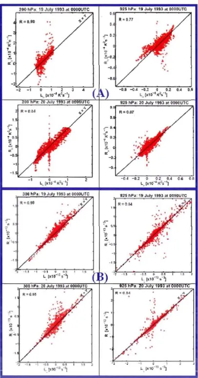
3.3. Spatial patterns of the internaI variabiIity tendency

Figure 5 presents the fields of the left-hand side term

(L

_o

(i,j,k,l»)

and the right-hand side term (R_o

(i,

j, k,

l»)

of the IV tendency equation for potential temperature (Eg. 14) at two pressure levels, each day from 18 to 21 July. We note good qualitative agreement between these two terms. To illustrate the correspondence

between them and to get a more quantitative evaluation, we present dispersion

diagrams in Figure 7A using al! grid points of the study domain (except the sponge

zone) for July 19 and 20, and we compute correlation coefficients. At the 200-hPa

25

respectively. On these same dates, the correlation coefficients at the 925-hPa level are

0.77 and 0.87, respectively (see Fig. 7A).

Figure 6 presents the corresponding fields of the left- and the right-hand side

terms of the IV tendency equation for relative vorticity (Eq. 19) at two pressure levels, each day from 18 to 21 July. Because relative vorticity is a noisier field than

potential temperature, so is the IV tendency. Nevertheless the results also show a

good qualitative agreement between the left- and right-hand side terms. Figure 78

shows the corresponding dispersion diagrams and correlation coefficients. On 19 July

1993, the correlation coefficients between these t\Vo telms are 0.90 and 0.84 at 300­

and 925-hPa levels, respectively; and on 20 July 1993, correlations are 0.88 and 0.84

at these same pressure levels, respectively.

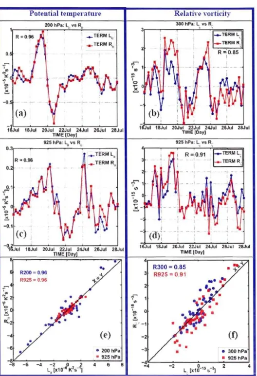
3.4. Time evolution of the domain-average internaI variability tendency

Next we compare in Figure 8 the time evolution of the left- and the right-hand

side terms during the period of interest, averaged over the selected domain (see Fig.

2a). The time evolutions denote fairly good agreement, with correlations coefficient

of 0.96 at 200 and 925 hPa for potential temperature, and 0.85 and 0.91 at 300 and

925 hPa, respectively, for relative vorticity. The diagnostics hence appears to provide

a fairly robust correspondence between the two components, Lif of the IV that developed in the 20-member ensemble and Rif that evaluates diagnostically the contributions to the IV using the archived data. So, we now proceed to analyse the

different contributions to the right-hand side term in order to gain sorne

understanding of the physical mechanisms responsible for the development and

evolution of IV in regional model simulations.

The previous results suggest that the developed tendency equations can be used

to understand the physical processes that lead to large IV in certain periods in the