This is an author-deposited version published in : http://oatao.univ-toulouse.fr/
Eprints ID : 8304
To link to this article : DOI:10.1109/TAES.2013.6404101
URL :
http://dx.doi.org/10.1109/TAES.2013.6404101
O
pen
A
rchive
T
OULOUSE
A
rchive
O
uverte (
OATAO
)
OATAO is an open access repository that collects the work of Toulouse researchers and
makes it freely available over the web where possible.
To cite this version :
Deudon, Francois and Bidon, Stéphanie and Besson, Olivier
and
Tourneret, Jean-Yves
Velocity Dealiased Spectral Estimators of
Range Migrating Targets using a Single Low
-
PRF Wideband
Waveform
.
(2013) IEEE Transactions on Aerospace and Electronic
Systems, vol. 49 (n° 1). pp. 244-265. ISSN 0018-9251
Any correspondence concerning this service should be sent to the repository
administrator: staff-oatao@listes.diff.inp-toulouse.fr
Velocity Dealiased Spectral
Estimators of Range Migrating
Targets using a Single Low-PRF
Wideband Waveform
FRAN ¸COIS DEUDON, Student Member, IEEE ST ´EPHANIE BIDON, Member, IEEE OLIVIER BESSON, Senior Member, IEEE JEAN-YVES TOURNERET, Senior Member, IEEE
University of Toulouse
Wideband radars are promising systems that may provide numerous advantages, like simultaneous detection of slow and fast moving targets, high range-velocity resolution classification, and electronic counter-countermeasures. Unfortunately, classical processing algorithms are challenged by the range-migration phenomenon that occurs then for fast moving targets. We propose a new approach where the range migration is used rather as an asset to retrieve information about target velocities and, subsequently, to obtain a velocity dealiased mode. More specifically three new complex spectral estimators are devised in case of a single low-PRF (pulse repetition frequency) wideband waveform. The new estimation schemes enable one to decrease the level of sidelobes that arise at ambiguous velocities and, thus, to enhance the discrimination capability of the radar. Synthetic data and experimental data are used to assess the performance of the proposed estimators.
This paper was presented in part at the IEEE Radar Conference, Washington, D.C., May 10—14, 2010.
Authors’ addresses: F. Deudon, S. Bidon, O. Besson, Department of Electronics, Optronics and Signal, University of Toulouse, ISAE, 10 Avenue Edouard Belin BP 54032, Toulouse, 31055, France, E-mail: (sbidon@isae.fr); J-Y. Tourneret, University of Toulouse, IRIT-ENSEEIHT-T´eSA, Toulouse, France.
I. INTRODUCTION AND PROBLEM STATEMENT Designing a nonambiguous radar mode, neither in range nor in velocity, is of great interest for radar operators. Indeed, prior to estimating both range and velocity of targets, a nonambiguous mode is very attractive as it allows targets to be discriminated from clutter, thereby enhancing detection probability. However, developing a nonambiguous mode is a challenging task as conventional radar systems (such as moving target indication (MTI) and coherent-pulse Doppler radars) are limited by the intrinsic relation that links the ambiguous velocity va to the ambiguous range Ra, i.e.,
Rava=¸0c
4 (1)
where ¸0 is the carrier wavelength and c is the speed of light. In other words one cannot lessen one type of ambiguity without worsening the impact of the other.
To alleviate this limitation classical radar systems send a series of bursts with multiple, pulse-repetition frequencies (PRFs) [1, 2]. As the range-Doppler locus of a scatterer depends on the PRF, using multiple PRFs may move the target out of the clutter, hence avoiding blind ranges or velocities. Numerous works have been published on that technique, e.g., [3]—[7]. However, using multiple PRFs presents several drawbacks. It requires a more complex postprocessing that may involve unfolding and correlation-like techniques. Also, the time on target is increased since several bursts are needed. A long dwell time is not very attractive as it precludes rapid wide coverage of the scene and may compromise the assumption of constant velocity for the target. Also, performance of the ambiguity removal process may be degraded in a multiple-target scenario [8].
Given the constant ongoing advances in RF hardware and signal processing, it is, nowadays, conceivable to design nonambiguous radar systems using a single PRF [9—13]. Such a mode is considered in our study. More precisely the work presented in this paper focuses on a radar system that uses a single low-PRF wideband waveform aimed at MTI operations. By wideband we mean that the fractional bandwidth is on the order of 10%; that is, the instantaneous bandwidth B represents 10% of the carrier frequency f0. Also, the bandwidth B is assumed to be large enough to give a range resolution ±R= c=(2B) of a few centimeters. On the other hand the low-PRF assumption for our radar system ensures that ranges of interest are nonambiguous, while Doppler frequencies are highly ambiguous. Hence, only Doppler ambiguities need to be resolved within this framework. This might be achievable thanks to the high range resolution (HRR) feature of the waveform as highlighted hereafter.
Unlike low range resolution (LRR), echo location systems, HRR radars are prone to the
well-known range-walk phenomenon. Indeed, due to the HRR, a moving point-target may not be confined anymore into a single range gate during the coherent processing interval (CPI). In other words, in wideband radar, the Doppler effect affects not only the carrier phase but also the complex envelope of the echoed signal. The faster the point-target, the greater the impact on its envelope. Several authors [8, 13—15] have shown that, for linear migration, the point-target signature can be easily expressed in the fast-frequency/slow-time domain. In such a case the fast-frequency domain is obtained by performing a Fourier transform on the fast-time limited to an LRR segment that contains the target (with allowance for range-walk). The point-target signature in the fast-frequency/slow-time domain can then be seen as a conventional bi-dimensional sinusoid–whose frequencies account, respectively, for the carrier-phase Doppler shift and the initial range of the target–and cross-coupling terms that account for range migration. These terms depend on the target velocity. Therefore, it is reasonable to think that, if carefully processed, they might bring enough information to resolve velocity ambiguities.
Thus, to obtain a nonambiguous mode in an HRR context, it is crucial to carefully design not only the transmitted waveform but also the processing of the received signal. HRR/MTI processing has to overcome several challenges. Among them, it has to suppress clutter and to take into account, simultaneously, the range-walk of a moving target, a possible spreading of the target over several adjacent range cells, and the presence of multiple targets in the LRR segment. Hereafter is given a succinct review about detection algorithms that have been applied and/or developed for HRR radars. We discuss them in light of their ability to suppress clutter and to remove velocity ambiguities.
Conventional Doppler processing has been tested for wideband signals, and it is obviously not satisfying as it does not take the range-walk of the target into account. On one hand it is unable to separate clutter from targets whose velocity is competing (modulo va) with the ones of the clutter; on the other hand, it leads to huge spreading and loss on the target peak [16].
In [10] the author underlines the inappropriateness of conventional Doppler processing for HRR radar. Instead, he proposes a two-step coherent algorithm. The first step aims at suppressing clutter in the fast-frequency/slow-frequency domain by a standard notch filter. Then, in the second step, the target energy is coherently integrated while testing the space of possible target speeds. Unfortunately, in the case of velocity ambiguities, the clutter suppression process induces some losses for aliased targets.
A single coherent integration processing allows the target gain to be recovered and velocity ambiguities to be moderated [8]. It can be implemented with a
fast algorithm based on a Keystone-like transform [17, 18]. The resulting range-Doppler map can be seen as an ideal point-target map blurred by a point spread function, i.e., the ambiguity function of the transmitted waveform. Several wideband ambiguity functions have been studied in the literature and may be used to estimate target features, such as the time delay and the radial velocity, see e.g., [16], [19]—[23]. However, though wideband ambiguity functions have the desirable property of transforming aliasing lobes into sidelobes, the level of these sidelobes remains high. This leads to two main drawbacks. First, a moving target can be hidden in or destructed by the sidelobes of another target. Secondly, the sidelobes’ level of clutter signal may be very high, even higher than that of a single moving scatterer. Indeed, given an LRR segment, clutter sidelobes from each range gate tend to add up via constructive interferences [24] (provided that the clutter signal is present at each range gate). In other words a simple coherent integration does not properly remove blind velocities. In [25], [26], a migrating target indicator (MiTI) is proposed to suppress clutter without introducing a specific loss for aliased targets. The essence of the MiTI is to discriminate the clutter signal as a nonmoving component in the received signal. More precisely the technique is based on the incoherent subtraction of range-velocity maps obtained from the coherent integration of two pulse subintervals. This method allows nonmoving components to be conveniently suppressed; nonetheless, the sidelobes of moving targets remain high.
Finally, in [14], the authors propose an iterative algorithm that suppresses clutter and estimates parameters of interest for an HRR target. The technique is extended in [15] to the case of multiple moving targets received on a phased array. In both cases the problem of velocity ambiguities is not taken into consideration.
In this paper, given the state-of-the-art, we are interested in developing methods that allow one to dealias the velocity by using a single low-PRF wideband waveform in the framework of HRR/MTI radars. To do so we propose a new complex spectral estimation algorithm aimed at decreasing the level of sidelobes that occur at ambiguous velocities. This technique is the direct continuation of the work presented recently in [27], where extended versions of the Capon and the APES filters have been proposed. Capon and APES algorithms are well-known adaptive filtering techniques used for complex spectral estimation in the case of narrowband signals [28—31]. For instance, they have been
successfully applied to narrowband synthetic aperture radar (SAR) data. In [27] wideband versions of both algorithms, namely the W-Capon and the W-APES, have shown similar trends as their narrowband counterparts, while alleviating, in part, the velocity
ambiguity. Unfortunately, the level of sidelobes remains high for fast moving targets, presumably due to an approximation of stationarity made during the derivation of the estimators. So as to overcome this restrictive approximation, we propose, here, an iterative process, based on the W-Capon, that allows one to fully take into account the range-walk of each point-target present in the scene. As explained later the principle is inspired by the CLEAN algorithm [32, 33]. We stress at this point that we are only interested in estimating, point-by-point, the complex amplitude of the range-velocity map. The final design of a constant false alarm rate (CFAR) detector is out of the scope of this work.
The remaining of the paper is organized as follows. In Section II the data model for the received signal is presented. Our interest focuses, more specifically, on a multiple point-target scenario. Note that the present study is restricted to the case where target motion can be neglected in the duration of a single pulse but not during the CPI. Within this framework the estimation problem of interest is formulated in Section IV. The W-Capon and the W-APES techniques are recalled, and the new iterative process based on the W-Capon estimator, is described. Finally, Section V studies the performance of these wideband spectral estimators. Analysis is performed with both synthetic data and experimental data provided by the Delft University of Technology (Tu-Delft) [34]. Conclusions are drawn in Section VI. II. DATA MODEL FOR WIDEBAND RADAR
This section introduces the data model for a wideband radar that sends a single series of coherent pulses with a low PRF. First, the model is restricted to a single point-scatterer with constant radial velocity. Then, the data model is extended to a more realistic scenario with internal receiver noise and where several targets may be involved.
A. Single Point-Target Model
A single point-target is considered here. It is shown that, after standard preprocessing operations (demodulation, down-conversion, and sampling), the signature of the echoed signal can be expressed in the fast-frequency/slow-time domain by a bi-dimensional sinusoid with cross-coupling terms.
1) Received Signal: The radar transmits a coherent burst of M pulses
stx(t) =
M¡1X m=0
up(t¡ mTr)ej2¼f0t (2)
where up(t) is the complex envelope of a single pulse, Tr is the pulse repetition interval (PRI), and f0is the carrier frequency. The envelope is assumed to have a duration T and a fractional bandwidth such that B=f0¼ 10%. If a moving point-scatterer is present in
the scenario, the signal received on the radar antenna can be approximated by a delayed and attenuated version of the transmitted signal (2), i.e.,
srx(t) = ®stx[t¡ ¿(t)] (3) where ® is the complex amplitude response of the target and ¿ (t) is its round-trip delay. Assuming that the radial velocity v of the target is constant during the CPI and small, with respect to the speed of light, the round-trip delay can be approximated by [35]
¿ (t) = ¿0¡2v
c t (4a)
with
¿0=2R0
c (4b)
where R0and ¿0are, respectively, the initial range and delay. Note that, by convention, positive velocity indicates that the target is moving towards the radar. Using (2) and (4a) in (3) leads to
srx(t) = ® MX¡1 m=0 up ·μ 1 +2v c ¶ t¡ ¿0¡ mTr ¸ £ exp · j2¼f0 μ 1 +2v c ¶ t ¸ (5) where constant phase terms have been (and will be systematically) absorbed into the complex amplitude ®.
As shown by (5) the received signal is affected by two main effects. First, the envelope up is translated by a delay that remains constant during the PRI: at the mth pulse the envelope is translated by a delay equal to ¿0+ mTr. Secondly, the Doppler effect, due to the relative motion of the target, distorts both the carrier and the envelope. Note that, contrary to the narrowband case, the effect on the envelope has to be considered. More precisely, as stated in the Introduction, we assume that the target range-walk is negligible during a single pulse but not during the whole CPI. This is tantamount to considering that the phase rotation 2¼B(2v=c)T is negligible while the phase rotation 2¼B(2v=c)MTr may not be, i.e.,
vT¿ ±R (6a)
and
vMTrÀ ±R (6b)
where the range resolution is given by ±R= c
2B: (7)
Finally, from (5), one recovers the usual physical phenomenon: if the target is moving towards the radar, the time scale is compressed, whereas, if it moves away, the signal is dilated.
2) Preprocessing: The received signal (5) is then successively down-converted to baseband, matched
filtered, and sampled. For notational convenience let us introduce the fast-time t0 and the slow-time mTr by making the following change of variables
t0= t¡ mTr:
After removing the carrier, the received baseband signal for the mth pulse is, thus, given by
sbb(t0, m) = ®up · t0¡ ¿0+2v c mTr ¸ £ exp · j2¼f02v c (t 0+ mT r) ¸ (8) where the target range remains constant over the pulse duration (i.e., assumption (6a)). The baseband signal is then range matched filtered, which is equivalent to cross-correlating, temporally, the signal (8) with the envelope up(t0), i.e.,
smf(t0, m) = Z +1
¡1
sbb(»)u¤p(»¡ t0)d»:
Using Parseval’s theorem and conventional properties of the Fourier transform, the matched filter output for the mth pulse is given in the fast-time/slow-time domain by smf(t0, m) = ® exp£j2¼f0(2v=c)mTr¤ £ exp£j2¼(2v=c)f0[¿0¡ (2v=c)mTr]¤ £ Z +1 ¡1 Up · f¡2v c f0 ¸ Up¤(f) £ exp£j2¼f[t0¡ (¿0¡ (2v=c)mTr)]¤df (9) where Up(f) is the Fourier transform of the complex envelope. Observing in (9) that the phase rotation (2v=c)2f
0MTr is negligible given the range of expected
target velocities and that the fractional bandwidth ensures that B=f0À 2v=c, the matched filter output boils down to smf(t0, m) = ® exp£j2¼f0(2v=c)mTr¤£ Z +1 ¡1 jUp (f)j2 £ exp£j2¼f[t0¡ (¿0¡ (2v=c)mTr)]¤df: (10) Then, assuming an ideal constant flat spectrum for the complex envelope, one has
smf(t0, m) = ® exp£j2¼f0(2v=c)mTr¤ £ Z B 0 exp£j2¼f[t0¡ (¿0¡ (2v=c)mTr)]¤df: (11) The analog-to-digital (A/D) converter that follows the matched filter samples the signal in the fast-time domain at a rate 1=B so that the digital signal to be
processed is, finally, for ` = 0, : : : , K¡ 1, smf μ ` B, m ¶ = ® exp£j2¼f0(2v=c)mTr¤ £ sinc ½ ¼ · `¡ μ `0¡vmTr ±R ¶¸¾ (12) where `0= ¿0B is the initial range gate of the
target and K is the total number of range gates approximately equal to K¼ BTr. Note that, given the wideband and the low-PRF assumptions, K might be quite large.
3) Signature in the Fast-Frequency/Slow-Time Domain: At this point it is appealing to express (12) in the fast-frequency/slow-time domain. To do so we notice, from (12), that the target component is mainly present in the range gate interval, e.g., for v¸ 0
½
`0¡v(M¡ 1)Tr ±R , : : : , `0
¾
(13) whose size is small compared with the total number of cells K. To coherently process the target, it is thus sufficient to focus our attention on a few range cells that contain the target, namely L range cells that define our LRR segment. Without loss of generality we assume that the target is confined in the first range gates ` = 0, : : : , L¡ 1. Then, the fast-frequency domain denotes the Fourier transform of the fast-time domain limited to this LRR segment. Hence, the target signal can be approximated in the fast-frequency/slow-time domain by
Smf(`, m)¼ ®exp£j2¼f0(2v=c)mTr¤
£ exp£¡j2¼[`0¡ (vmTr=±R)](`=L)
¤ (14) where ` stands for the subband index.
Given (14) the signature of a point-target in the fast-frequency/slow-time domain can be summed up in matrix A of size L£ M, whose (`,m)th element is given by
[A]`,m= ej2¼fr`ej2¼fDmej2¼¹fD`m for ` = 0, : : : , L
¡ 1 m = 0, : : : , M¡ 1
(15) where fr and fD stand, respectively, for the
range-frequency and the Doppler frequency, i.e., fr=¡`0
L (16a)
fD= f02v
c Tr (16b)
and ¹ is a constant coefficient that stands for the “fractional bandwidth per subband”
¹ =B=L
Fig. 1. Amplitude (modulus only) of migrating point-target. (a) Fast-time/slow-time domain. (b) Fast-time/slow-frequency domain. (c) Fast-frequency/slow-time domain. (d) Fast-frequency/slow-frequency domain. Scenario parameters: v = 2:1va, `0= 64, L = 128,
M = 128, ¹ = 7:8£ 10¡4.
Note that, in the following, we use the vectorized version of the target signature, i.e.,
a = vecfAg (18) where vecfg is the operator that stacks column by column the matrix inside the bracket.
4) Interpretation of the Target Signature:
Observing (15) the target signature can be interpreted as a bi-dimensional sinusoid with frequency (fD, fr) and cross-coupling terms that account for the range migration. To fully understand the meaning of (15), the modulus of the amplitude for a moving target with unit amplitude is depicted in Fig. 1 in four different domains. These domains are obtained by standard Fourier and inverse-Fourier transforms applied to (15).
a) In the fast-time/slow-time domain (Fig. 1(a)), the range gate of the target is described by a line whose equation is given by
tfast(m) =¡L[fr+ ¹fdm] =R0 ±R ¡
vTr
±Rm: (19) Hence, the linear migration and the initial range-gate imposed by Assumption (4a) are both recovered. Note that the faster the scatterer, the higher the slope vTr=±R, and consequently, the greater the number of range bins crossed by it.
b) In the fast-frequency/slow-frequency domain (Fig. 1(d)), for a given subband ` the classical target signature for narrowband radar is recovered with a
slow-frequency equal to fslow(`) = fD(1 + ¹`) = f02v c Tr+ 2v c B LTr`: (20) Hence, a range migration in the fast-time/slow-time domain results in a “slow-frequency migration.” The faster the target, the wider the bandwidth occupied in the slow-frequency domain. Note that (20) refers to the slow-frequency that has been unfolded.
c) In the fast-time/slow-frequency domain (Fig. 1(b)), the target peak is spread over a rectangle. Note that this is the target response to conventional Doppler processing. The faster the target, the greater the spreading. Moreover, the target location may be aliased over the slow-frequency due to the low PRF.
d) Finally, in the fast-frequency/slow-time domain (Fig. 1(c)), the modulus of the target amplitude is constant.
B. Multi-Target Scenario
In Section II-A our attention has been limited to the case of a single point-target. From now on a more realistic scenario is considered, where multiple scatterers are present in the scene and where the internal receiver noise is also taken into account. We denote by Z the data matrix of size L£ M that is obtained after applying 1) standard preprocessing operations, 2) a selection of L range gates, and 3) a range-Fourier transform as depicted in the
Fig. 2. Flowchart: standard preprocessing+selection of L cells+range transform.
flowchart of Fig. 2. The vector z = vecfZg denotes the vectorized version of the matrix Z.
In the following it is assumed that the received signal z contains the response of Ntscatterers embedded in thermal noise
z =
Nt
X
t=1
®tat(!D,t, !r,t) + n (21) where ®t and at are, respectively, the amplitude and the signature of the tth point-scatterer with frequency pair (!D,t, !r,t)1and where n is the internal
receiver noise. The noise sequence n is modeled as a zero-mean complex Gaussian distribution CN (0,¾2I
LM), where ¾2is the noise power. We
assume in this work that the diffuse part of the clutter, if any, has been filtered in the preprocessing operations with standard techniques using, for instance, secondary data obtained from adjacent LRR segments to the one of interest, e.g., [36].
In the remainder of the paper, we are interested in estimating the complex amplitudes ®ts of the Nt scatterers introduced in (21). Three new wideband spectral estimators are presented and studied for different scenarios.
III. FORMULATION OF THE ESTIMATION PROBLEM In order to formulate the problem of estimation, we follow the lines of [29] (where the APES estimator is derived) while taking into account the specificities of the wideband context. Given the problem of interest, the maximum-likelihood (ML) principle is invoked in order to build new adaptive spectral
1To obtain more compact expressions, the target signature can be expressed with respect to !r= 2¼frand !D= 2¼fD.
estimators. Prior to designing such estimators, and to motivate our study, we present the performance of an approximate ML estimator that would be obtained in the clairvoyant case. This estimator corresponds to a quasi-optimal case and is the reference for comparing the performance of other estimators.
A. Analysis Model
Let us consider the bi-dimensional data-sequence
Z defined previously in (21). As in [29] we intend
to estimate, for all frequency pairs (!D, !r), the amplitude of a wideband target that may be present at this frequency. To do so the following data model is assumed for m = 0, : : : , M¡ 1 and for ` = 0,:::,L ¡ 1
[Z]`,m(!D, !r) = ®(!D, !r) exp£j(m!D+ `!r+ m`¹!D)¤ + e`,m(!D, !r) (22) where ®(!D, !r) is the complex amplitude of a
target at frequency (!D, !r) and where e`,m(!D, !r) represents the unmodeled and undesired components at this frequency. Note that, as we wish to alleviate the velocity ambiguities in a low-PRF context, the frequency range of interest is given by
¡!r 2¼2 [0,1] (23a) !D 2¼ 2 h ¡nva 2 , nva 2 i (23b) where nva2 N¤ is the maximum Doppler ambiguity factor expected for a target. In other words nvais the smallest integer that verifies
jvmaxj ·
nvava 2
where vmax is the maximum velocity expected for a target.
As done in [29] a new data set is created from the initial sequence Z. More precisely a sliding window of size ¯L£ ¯M is applied to Z so as to obtain NLNM submatrices with NL= L¡ ¯L + 1 and NM= M¡ ¯M + 1. Each submatrix is then vectorized into an
¯
L ¯M-length vector denoted by zp,q. Further following the procedure of [29], each snapshot can be expressed as [27]
zp,q= ®ap,q+ ep,q (24) for p = 0, : : : , NL¡ 1 and q = 0,:::,NM¡ 1 and where the dependency on (!D, !r) is not explicitly written in order to lighten the expression and where
ap,q= ej!Dqej!rpej¹!Dpq¯a ¯ fb
p− cqg (25a)
bp= [1 ej¹!Dp: : : ej¹!Dp( ¯M¡1)]T (25b)
cq= [1 ej¹!Dq: : : ej¹!Dq( ¯L¡1)]T: (25c)
In (25a) the vector ¯a represents the substeering vector for the (0, 0)th sliding window, i.e., the vectorized
matrix A described by (15) when its size is reduced to ¯
L£ ¯M. The symbols¯ and − refer to the Hadamard and the Kronecker matrix products, respectively. Finally, note that the cross-coupling terms ej¹!D`m that
account for the range migration in (15), result in the term ej¹!Dpqb
p− cqfor the snapshot zp,q.
In the following it is assumed, as in [29], that the complex amplitude ® is an unknown deterministic quantity, and that the noise vectors ep,q are centered, independent (hence mutually uncorrelated), and distributed according to a complex Gaussian distribution, i.e.,
ep,q» CN (0,Qp,q) (26a) and
Efep,qeHr,sg = Qp,q±p,r±q,s (26b)
where Qp,q is the ¯L ¯M£ ¯L ¯M covariance matrix of the snapshot ep,q. Given (26), two important remarks are in order. First, the hypothesis of independence is very strong and is rigorously not correct as two adjacent windows are highly overlapped. However, the same assumption is made in [29] and allows one, in any event, to design efficient estimators for the complex amplitude in the narrowband case. We thus follow this path here. Secondly, it is worth noticing that the matrices Qp,qare highly likely to be nonstationary. In other words these matrices may actually depend on the window indices p and q. For instance, consider the simplified scenario where ep,qwould consist of a single point-scatterer with frequency ( ˜!D, ˜!r). The noise covariance matrice of the (p, q)th window would then be given by
Qp,q/ f¯a( ˜!D, ˜!r)¯a( ˜!D, ˜!r)Hg ¯ f(bp( ˜!D, ˜!r)bp( ˜!D, ˜!r)H)
− (cq( ˜!D, ˜!r)cq( ˜!D, ˜!r)H)g (27)
where the symbol/ means proportional to. In the narrowband context, i.e., ¹ = 0, the range migration is not present and only the first term of (27) remains so that the matrices Qp,q are all equal [29]. Here, the range migration prevents the matrices from being equal. The faster the moving scatterers in Qp,q, the greater the nonstationarity of the matrices Qp,q. B. ML Estimation in the Clairvoyant Case
Let us remind the reader that our goal is to estimate the deterministic amplitude ® for each frequency (!D, !r) given the problem described by (24) and (26). At this point we propose developing estimators of ® based on the ML principle. To
motivate the work presented in the following sections, we focus our attention first on the clairvoyant case, that is, when the noise covariance matrices Qp,qare known exactly.
1) Clairvoyant Case: Given the problem (24) and (26), the ML estimator of ® in the clairvoyant case is defined by
ˆ
®clair= arg max
® ¤(fzp,qg j ®,fQp,qg)
where ¤( ) is the log-likelihood function. According to the estimation problem previously described, the log-likelihood (up to a constant factor) is given by
¤(fzp,qg j ®,fQp,qg) =¡X p,q ln(jQp,qj) ¡X p,q (zp,q¡ ®ap,q)H £ Q¡1p,q(zp,q¡ ®ap,q) (28)
wherej:j is the determinant of a matrix. The argument ® that maximizes (28) minimizes as well the
expression X p,q (zp,q¡ ®ap,q)HQ¡1p,q(zp,q¡ ®ap,q) =X p,q zHp,qQ¡1p,qzp,q¡ ¯ ¯ ¯Pp,qaHp,qQ¡1p,qzp,q ¯ ¯ ¯2 P p,qaHp,qQ¡1p,qap,q +X p,q aHp,qQ¡1p,qap,q£ ¯ ¯ ¯ ¯ ¯®¡ P p,qaHp,qQ¡1p,qzp,q P p,qaHp,qQ¡1p,qap,q ¯ ¯ ¯ ¯ ¯ 2 : Consequently, the ML estimator of ®, for known matrices Qp,q, can be easily expressed in closed form by the ratio ˆ ®clair= P p,qaHp,qQ¡1p,qzp,q P p,qaHp,qQ¡1p,qap,q : (29)
To illustrate the performance of the clairvoyant estimator in a realistic radar scenario, we define an approximate ML estimator where the covariance matrices Qp,q in (29) are replaced with the matrices
Rp,q defined by
Rp,q=Efzp,qzH
p,qg: (30)
More specifically the correlation matrices Rp,qare built according to the generation model (21), i.e.,
Rp,q= Nt X t=1 j®tj2atp,qa H tp,q+ ¾ 2I ¯ L ¯M: (31)
Plugging (31) into (29), one obtains finally ˆ ®a-clair= P p,qaHp,qR¡1p,qzp,q P p,qaHp,qR¡1p,qap,q : (32)
2) Performance in Clairvoyant Case: To illustrate the potential of the estimator (32), we consider a simple scenario where two point-targets are present. Both targets have the same complex amplitude and initial range but different velocities. More precisely
Fig. 3. Spectral estimates. (a) Coherent integration. (b) ML estimator of ® when covariance matrices Rp,q are known. Scenario parameters: L = 16, M = 16, ¹ = 0:0063, target 1 (v1, `0,1) = (0:5va, 8),j®1j2= 1, target 2 (v2, `0,2) = (1:5va, 8),j®2j2= 1, thermal noise
power ¾2= 0:01.
it is assumed that their velocities are one ambiguous velocity va apart. We compare the spectral estimates obtained with (29) with the spectral estimates obtained from a simple coherent integration2[8, 18], i.e.,
ˆ
®coh-sum= a
Hz
aHa (33)
where a is the steering vector (18) with frequency (!D, !r). Note that the range-velocity map for (33) is computed with the fast-algorithm described in [18].
Figure 3 shows the modulus of the spectral estimates obtained from both spectral estimators (32) and (33). From both range-velocity maps, several observations can be made. First, (33) is not an efficient spectral estimator as can be seen in Fig. 3(a). Indeed, the use of the coherent summation method results in high sidelobes and wide peaks. For this specific scenario mainlobe and sidelobes of both targets are not identifiable. Unlike the estimator (33) the clairvoyant estimator (32) accurately restores the amplitude of the targets, reduces the mainlobe width, and suppresses the sidelobes. Note that the range-velocity resolution is thus drastically increased. Also, the average level of the scatterer-free domain is decreased as compared with the one observed with the coherent integration.
The spectral estimator (32), and implicitly (29), are thus appealing techniques that can alleviate velocity ambiguity of point-targets for wideband radar. Unfortunately, such estimators cannot be implemented in practical cases. In order to circumvent
2Note that the coherent summation in a wideband context is the counterpart of the fast Fourier transform (FFT) for narrowband signals.
this drawback, we propose, in the following section, developing adaptive versions of the clairvoyant estimator (29).
IV. ADAPTIVE SPECTRAL ESTIMATORS
In this section we describe three new spectral estimators that are adaptive versions of the clairvoyant ML estimator (29) for wideband radar. As discussed previously (29) relies on the knowledge of the noise covariance matrices Qp,q. In this section we consider that there is no prior knowledge about the matrices
Qp,q that have to be estimated from the observed data setfzp,qg. Unfortunately, for each matrix Qp,q we have access only to a single realization, i.e., the subvector
zp,q. To overcome this problem two strategies are proposed hereafter. The first strategy simplifies the problem by assuming that the matrices Qp,qare equal to a common matrix Q. This matrix Q is then estimated by using the observation vectors zp,q. This leads to two spectral estimators, the W-Capon and the W-APES. The second strategy accounts for the nonstationarity of the noise covariance matrix, one scatterer after another. To do so an iterative process, based on the W-Capon, is developed.
A. Stationary Assumption
We assume herein that the noise covariance matrices Qp,q are equal to a common covariance matrix, i.e.,
Qp,q= Q, 8p,q: (34)
Given the initial problem (24), this is tantamount to taking into account the nonstationarity of the target under test ap,q at the frequency of interest (!D, !r), while neglecting the nonstationarity of the noise vector ep,q. In this case the normalized log-likelihood
(28) reduces to ¤(fzp,qg j ®,Q) =¡ln(jQj) ¡ tr ( Q¡1 1 NMNL X p,q (zp,q¡ ®ap,q)(zp,q¡ ®ap,q) H ) (35) where trfg stands for the trace of the matrix between brackets. From (35) two spectral estimators based on the ML principle are presented hereafter [27]. Note that the hypothesis of stationarity (34) is not valid in a scenario with fast-moving scatterers and/or in case of numerous moving scatterers.
1) W-APES: The first spectral estimator presented here is the conventional ML estimator of ® that maximizes (35). This estimator is referred to as the W-APES and is defined by
ˆ
®wapes= arg max
® ½ max Q ¤(fzp,qg j ®,Q) ¾ : (36) It is shown in the Appendix that solving (36) is tantamount to minimizing a cost function that belongs to a class of problems that does not seem to have a closed-form solution [37, 38]. Usually, standard optimization techniques are used to obtain the solution. In this paper, to avoid the eigendecomposition (54) introduced in the Appendix and required for each frequency pair (!D, !r), an iterative approach is invoked instead [39]. More specifically an iteration is set between the two partial derivatives of (35)–with respect to ® and to Q–that have been equated to zero
® = P p,qaHp,qQ¡1zp,q P p,qaHp,qQ¡1ap,q (wapes1) Q = 1 NMNL X p,q (zp,q¡ ®ap,q)(zp,q¡ ®ap,q)H: (wapes2) While initializing the iteration (wapes1)—(wapes2) by setting Q = ˆR, where ˆR is the sample correlation
matrix ˆ R = 1 NMNL X p,q zp,qzHp,q (37) no problem of convergence has been encountered in our simulations.
2) W-Capon: Herein, we propose deriving a second adaptive version of the spectral estimator (29) that is less complex than (36). Within the
narrowband framework it is possible to use a two-step procedure that results in the Capon estimator [29]. We apply a similar two-step procedure here for the wideband context and denote by W-Capon the resulting estimator. In the first step, the ML estimator of ® is derived with respect to the problem given by (24), (26), and (34) while assuming that the noise
covariance Q is known. Then, in a second step, the matrix Q is replaced by the sample correlation matrix ˆR (37). Following this procedure it is
straightforward to show that the W-Capon estimator can be expressed as ˆ ®wcapon= P p,qaHp,qRˆ¡1zp,q P p,qaHp,qRˆ¡1ap,q : (38)
Contrary to the W-APES estimator (36), the W-Capon estimator (38) has a closed-form expression.
Moreover, its computation requires only one matrix inversion that does not depend on the frequency of interest (!D, !r). This makes the W-Capon method very interesting in terms of computational complexity. REMARK1 If the alternate maximization proposed in Section IV-A.1 to derive the W-APES (56) is initialized with Q = ˆR, the first iteration of this
maximization (wapes1) yields the W-Capon estimator. 3) Limits of the W-Capon and W-APES Estimators: In Sections IV-A.1 and IV-A.2, we propose two new adaptive spectral estimators designed for wideband radar signals. Both are derived under the assumption of a stationary noise covariance matrix while taking into account the migration of the target under test. As shown in Section V, these estimators are acceptable for relatively slow targets. In this case, the height and width of the spectral peaks are reasonable, while sidelobes remain relatively low. However, for faster targets, sidelobes become very high. In the next section a new method is proposed to further enhance the spectral estimation performance when the stationarity assumption is not satisfied.
B. Nonstationary Assumption
We propose herein a third adaptive version of the spectral estimator (29) considering the migration of the target under test but also the migration of each scatterer present in the scenario. After presenting the principle of the new estimation technique, the procedure is carefully detailed step-by-step. Finally, important remarks about the proposed algorithm are highlighted. As explained hereafter the estimator assumes that the number of scatterers Nt in the scenario is small enough to ensure a certain level of sparsity in the range-velocity map. This assumption is not especially made for the W-APES and W-Capon estimators.
1) A CLEAN-Like Method: In a first attempt to take into account the migration of every scatterer present in the scene, we propose to simplify the estimation problem by replacing in (29) the matrices
Qp,q with the estimates of the matrices Rp,qderived using a specific structure inspired by (31). We see in Section III-B that, in the clairvoyant case, i.e., for known matrices Rp,q, this leads to appealing
estimation strategies. The spectral estimator proposed herein is referred to as the iW-Capon estimator and is defined as follows ˆ ®iwcapon= P p,qaHp,qRˆ¡1p,qzp,q P p,qaHp,qRˆ¡1p,qap,q (39)
where ˆRp,qis a structured matrix estimator for Rp,q given by ˆ Rp,q= ˆ Nt X t=1 j ˆ®tj2ˆatp,qˆa H tp,q+ ˆRn (40) where ˆ
Nt is the estimated number of point-scatterers in the scene;
ˆ
®t is the complex amplitude of the tth point-target; ˆatp,q is the steering subvectors of the tth point-target with estimated frequency ( ˆ!D,t, ˆ!r,t);
ˆ
Rnis the unstructured covariance matrix that refers to the stationary noise component which does not depend on the indices (p, q).
In this paper we assume that the number of scatterers Nt is exactly known so that ˆNt= Nt (this assumption is discussed later). To estimate the other parameters involved in the estimator of Rp,q(40), we adopt the following reasoning. In relatively sparse-scatterer scenarios, we have observed that in the range-velocity map obtained from a W-Capon estimation (38), the brightest point corresponds to the position of a true point-target. In other words we assume that the brightest spot is not the result of constructive interferences of sidelobes from other scatterers (similar assumption is made for the CLEAN algorithm [33]). From this observation we propose to refine the estimation of Rp,q in the following way. The structured nonstationary part of the estimator (40) is assumed to be temporarily due to one scatterer, i.e., Nt= 1, and it is built from the estimated complex amplitude and frequency pair of the brightest point. The unstructured stationary part ˆRnis built as the sample correlation matrix of a new data set that is estimated from the initial set
z from which the first estimated scatterer has been
removed. The correlation matrices Rp,q are thus “de-stationarized” with respect to the first point-target. To continue we propose to derive a new W-Capon range-velocity map (38) with these de-stationarized matrices Rp,q. By doing so we hope that the sidelobes of the brightest target will be drastically reduced. The two brightest points of this map can then be used to de-stationarize (40), assuming temporarily that Nt= 2. The process can then be repeated Nt times until each point-target has been taken into account in order to estimate the structured nonstationary part of the estimator (40).
To sum up we propose to set an iterative process (with Nt iterations) to estimate the matrices Rp,q. Each iteration can be decomposed in two main steps. First step: a W-Capon-like estimation procedure is applied to the initial data vector z.
Second step: the sample covariance matrices ˆRp,qare updated.
By updating, we mean that at each iteration, the nonstationarity of the matrices Rp,q is taken into account for one more scatterer. Note that the iterative W-Capon (iW-Capon) algorithm is similar to a CLEAN procedure [32, 33].
2) Iterative Procedure: Herein we detail the proposed iW-Capon algorithm, which computes the estimators (39) and (40) iteratively. After an initialization step, Ntiterations are performed so as to de-stationarize the matrices Rp,q one scatterer after another. Note that for the sake of clarity, the dependence on the frequency pair (!D, !r) is sometimes reintroduced. The bi-dimensional domain ID£ Ir represents the frequency points considered for
the spectral analysis. It is required that this grid be thin enough to obtain good results. Also, to correctly initialize the algorithm, it is assumed that within this domain, the scatterers map is sparse enough to ensure that the brightest point in the W-Capon map corresponds to a true scatterer.
b) Initialization: First, the algorithm is initialized by assuming that the correlation matrices ˆRp,qequal the stationary solution, i.e.,
ˆ
R(0)p,q= ˆR (41) where ˆR has been defined in (37).
b) Iterations for i = 1 to Nt: The ith iteration aims to take into account the range-migration of the i brightest point-targets. Each iteration can be decomposed in two main steps.
Step 1 W-Capon-like estimation applied to z In the first step a W-Capon-like estimation (38) is applied to the initial data setfzp,qg but with modified matrices ˆRp,q. More specifically, for all (!D, !r)2 ID£ Ir, a W-Capon-like estimate is computed as
follows ˆ ®(i)(!D, !r) = P p,qaHp,q(!D, !r)[ ˆR(ip,q¡1)]¡1zp,q P p,qaHp,q(!D, !r)[ ˆR(i¡1)p,q ]¡1ap,q(!D, !r) : (42) The expression (42) is directly obtained from (38) by replacing the correlation matrix ˆR by the matrices
ˆ
R(i¡1)p,q obtained at the previous iteration (i¡ 1). The estimates ˆR(i¡1)p,q are assumed to have a nonstationary part due to the i¡ 1 brightest scatterers and a
indices (p, q). Note that for i = 1, the first step reduces to a W-Capon map computation.
Step 2 Updating of the covariance matrices ˆRp,q
In the second step the covariance matrices ˆRp,qare updated. The matrices ˆR(i)
p,q are estimated by taking
into account the migration of an additional scatterer, i.e., the ith brightest scatterer. To do so the following steps are proposed.
Step 2.1 Estimation of the nonstationary part of ˆR(i)
p,q First, to update the matrices ˆR(i)p,q, we estimate
the nonstationary part of the matrices that correspond to the i brightest spots in the range-velocity map (42). Hence, we are searching for the i first local maxima in the map defined by
( ˆ!D,t(i), ˆ!r,t(i)) = arg maxt
(!D,!r)2ID£Ir
j ˆ®(i)(!
D, !r)j2 (43)
for t = 1, : : : , i, where maxk denotes the kth local maximum in decreasing order (thus max1 is the global maximum). The amplitude and signature of the i brightest targets are then estimated, respectively, by
ˆ
®(i)t = ˆ®(i)(!(i)D,t, !(i)r,t) (44a) ˆa(i) t = a(! (i) D,t, ! (i) r,t): (44b)
Step 2.2 Estimation of the stationary part of ˆR(i) p,q
To fully update the matrices ˆR(i)
p,q, we estimate their
stationary part that corresponds to the Nt¡ i remaining scatterers plus white noise. We create a new data vector z(i) that is exempt from the components ˆ®(i)t ˆa(i)t
by successively projecting z onto their orthogonal subspaces z(i)= i Y t=1 P(i)t z (45)
where P(i)t is defined as
P(i)t = ILM¡ˆa (i) t ˆa (i)H t ˆa(i)H t ˆa(i)t : (46)
A new data setfz(i)
p,qg is then created by applying a
sliding window of size ¯L£ ¯M to the vector (45). The stationary part of ˆR(i)
p,qis estimated by ˆ R(i) n = 1 NLNM X p,q z(i) p,qz(i) H p,q: (47)
Step 2.3 Computation of the matrices ˆR(i)
p,q Finally,
the matrices ˆR(i)
p,qare computed as the sum of the
structured nonstationary component defined by (44) and the stationary component (47), i.e.,
ˆ R(i)p,q= i X t=1 j ˆ®(i) t j 2ˆa(i) tp,qˆa (i)H tp,q + ˆR (i) n : (48)
As the matrices ˆR(i)
p,qtake into account the migration
of the i brightest scatterers (and given the performance obtained in the clairvoyant case), a range-velocity map (42) derived with (48) is intended to show i thin peaks with very low sidelobes, i.e., the i brightest spots, and to show Nt¡ i peaks with secondary sidelobes.
c) End of the iterations: At the end of the Nt iterations, the matrices ˆR(Nt)
p,q take into account the
migration of the Nt scatterers in the scenario, thus we set (40) to
ˆ
Rp,q= ˆR(Nt)
p,q:
If the estimation scheme is efficient enough, the final range-velocity map derived from these matrices will show Nt peaks with very low sidelobes.
3) Remarks about the iW-Capon Estimator: Important remarks can be made concerning the implementation of the iterative iW-Capon algorithm.
a) Additional step to enhance estimation: To improve the estimation of (44), a modification is brought to the iterative process described in Section IV-B.2. At the ith iteration step 1 (42) and step 2 (48) of the algorithm are repeated until the i amplitude estimators converge. More specifically denote as j the index of the “subiteration” between (42) and (48) at the ith iteration, and introduce the i£ 1 vector
ˆ
®(i)j = [ ˆ®(i)1,j: : : ˆ®(i)i,j]T
that contains the complex amplitude estimates of the i brightest spots at the jth subiteration. Convergence is declared when the following practical convergence criterion is met k ˆ®(i)j ¡ ˆ® (i) j+1k 2 · ²
where ² is the convergence threshold defined by the radar operator.
b) Determining Nt: While describing the iW-Capon algorithm, we assume that the number of scatterers Nt is exactly known. In practical cases, this number has to be estimated. Though not studied here this could be done via a generalized Akaike information criterion as proposed in [15] or by using an adaptive whiteness criterion to stop the algorithm. In any event a robustness analysis should then be conducted to assess the effect of an underestimation and overestimation of Nt.
c) Sparse scenario: Finally, we stress that the iW-Capon is based on the assumption that the Ntbrightest spots in the range-velocity domain correspond to true point-target and are not the result of sidelobe constructive interferences. Such an assumption is not made for the W-Capon and the W-APES estimators.
V. NUMERICAL SIMULATIONS
This section studies the performance of the proposed wideband spectral estimators W-APES,
TABLE I Scenario Parameters Waveform carrier f0 10 GHz bandwidth B 1 GHz PRI Tr 1 ms pulses M 16 fractional bandwidth B=f0 10% range resolution ±R= c=(2B) 15 cm ambiguous velocity va= cfr=(2f0) 15 m/s Ranges of Interest LRR segmenta L 16 Internal Receiver Noise
power ¾2 0.01
aMore precisely, L is a preprocessing parameter.
W-Capon, and iW-Capon. Wideband synthetic data are first considered for sparse-target scenarios exempt from clutter. Then, the wideband spectral estimators are applied to experimental data collected from the PARSAX radar.
A. Synthetic Data Exempt from Clutter A synthetic scenario exempt from clutter is
considered in this section. We intend to show a simple example where the proposed wideband estimators can alleviate the velocity ambiguity of point-targets with a single pulse contrary to narrowband techniques. After precising the simulation parameters, the range-velocity maps obtained from the spectral estimators of interest are compared.
1) Scenario:
a) Data: The received signal z is generated in the fast-frequency/slow-time dimension according to the wideband model (21). The radar considered has a 10% fractional bandwidth with a range resolution of ±R= 15 cm and a PRF of 1 kHz. Two point-targets, a slow target and a fast target, are introduced in the scene in two different ways. In the first case aliased lobes (obtained from narrowband techniques) of both scatterers do not compete in the range-velocity map as depicted in Fig. 4(a) and (b). In the second case aliased lobes do compete as seen in Fig. 5(a) and (b). For each point-target t the signal-to-noise ratio (SNR) is defined as SNRt= 10 log10 ½ j®tj2 ¾2 ¾ : (49)
High SNR values are considered here. Useful parameters for data generation are summed up in Tables I and II.
b) Processing parameters: Algorithms that require forming a new data set from z via a sliding window have the same window size ( ¯L, ¯M) for the simulations. Note that for the iW-Capon algorithm, the number of
TABLE II
Scenario Parameters: Point-Targets
Target 1 Target 2 power jatj2 1 1 velocity vt(m/s) 7.5 22.5 initial range gate `0,t ½ 4a
8¡ 0:8b 8 Doppler fD,t= vt=va 0.5 1.5 range frequency fr,t ½¡0:25a ¡0:45b ¡0:5 range gate walk vtMTr=±R 0.8 2.4 aFirst case scenario: noncompeting targets.
bSecond case scenario: competing targets.
TABLE III Processing Parameters
APES, Capon, W-APES, W-Capon, iW-Capon sliding window size ( ¯L, ¯M) =
³L 4, M 4 ´ 2D-grid ID= n ¡n2va, 1 4M, : : : , nva 2 ¡ 1 4M o Ir= n 0, 1 4L, : : : , 1¡ 1 4L o unfolding factor nva= 6 iW-Capon convergence parameter ² = 10¡3
targets is supposed to be known, i.e., the procedure is stopped at the Ntth iteration. Useful parameters used for processing are reported in Table III.
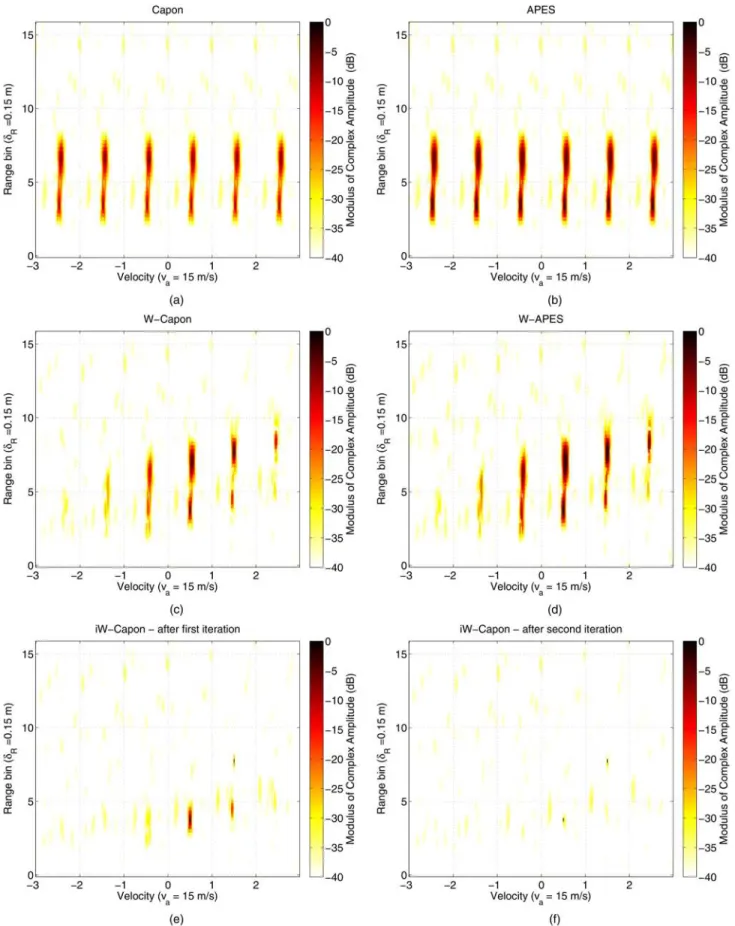
2) Range-Velocity Maps: Range-velocity maps obtained from the wideband spectral estimators, i.e., the W-APES (56), W-Capon (38), and iW-Capon (39), are compared with two narrowband estimators, namely the Capon and APES estimators [28, 29]. Note that all figures show the amplitude modulus.
Amplitude estimates obtained for the first case scenario are depicted in Fig. 4. We recall that for this scenario, two noncompeting targets are put in the scene. The following remarks can be made accordingly.
Estimation of target positions. From Fig. 4(a) and (b), it is clear that the positions of the target peaks, estimated from the Capon and the APES estimators, are shifted off their true location. Indeed, Capon and APES estimators coherently integrate the target under test while ignoring its possible migration. This leads to a spreading of the target response peak in the fast-time/slow-frequency. The same phenomenon is underlined earlier with simple Doppler processing in Fig. 1(b). Unlike narrowband spectral estimators, W-Capon, W-APES, and iW-Capon estimators coherently integrate the target under test while
Fig. 4. Comparison of spectral estimates for synthetic scenario with two noncompeting scatterers (v1, `0,1) = (0:5va, 4), (v2, `0,2) = (1:5va, 8). (a) Capon. (b) APES. (c) W-Capon. (d) W-APES. (e) iW-Capon, map after first iteration. (f) iW-Capon, map after
taking into account its migration. It can be observed in Figs. 4(c), (d), and (f) that the resulting target positions are estimated correctly.
Estimation of target amplitudes. Capon and APES do not properly estimate the amplitude of wideband targets. This is also due to the spreading of the migrating target response peak. W-Capon, W-APES, and iW-Capon provide better amplitude estimates. As in the narrowband case, the W-Capon estimator tends to underestimate the target amplitude, while W-APES and iW-Capon restitute a more accurate value.
Width of targets peaks. Peak widths are much wider for narrowband algorithms as they do not take range migration into account. As for the wideband estimators, the W-Capon method provides narrower peaks than that of the W-APES (the same trend has been observed for their narrowband counterparts [29]). Note that the iW-Capon estimator yields thinner peaks iteration after iteration. More precisely, as expected at the end of the ith iteration, the i brightest spots are taken into account into the matrices Rp,q, and their corresponding sidelobes almost vanish. This tends to prove that, for an efficient estimation, not only the migration of the target under test has to be considered but also the migration of the other scatterers present in the scenario.
Velocity dealiasing. The APES and the Capon methods give periodic maxima with respect to the velocity. Indeed, they are not designed to alleviate velocity ambiguity so that aliased lobes occur along the velocity axis. On the contrary our wideband spectral estimators take advantage of the additional information about target velocity brought by the cross-coupling terms in (15). By doing so aliased lobes are turned into sidelobes. Sidelobe heights of the W-APES and the W-Capon methods are moderate for slow moving targets, but they remain high for fast targets. The W-Capon has lower sidelobes than the W-APES. As for the iW-Capon estimator, the sidelobes vanish iteration after iteration, which is a very appealing property. Numerical values for the relative height of the first sidelobe observed for the slowest target are, respectively, given for the W-APES, W-Capon, and iW-Capon by¼ ¡8:5 dB, ¼ ¡14 dB, none. For comparison purposes the relative level of the first sidelobe with a coherent integration algorithm would be equal to f0=(BM)¼ ¡4 dB [18].
Amplitude estimates obtained for the second case scenario are depicted in Fig. 5. We recall that this scenario is defined by two competing targets. The following remarks can be made accordingly.
1) Previous observations concerning target location still hold for this scenario.
2) Peak widths and sidelobes increase for each algorithm. Also, the average level of the scatterer-free region is slightly higher than previously observed in Fig. 4.
3) Peak heights are strongly affected for the narrowband estimators as well as for the W-Capon and the W-APES techniques, as seen in Figs. 5(c) and (d). For instance, the peak of the slowest target is clearly underestimated. This is certainly the result of destructive interferences between the mainlobe of the slow target and the sidelobes of the fast target.
4) On the contrary, after one iteration of the iW-Capon procedure (see Fig. 5(e)), the sidelobes of the first detected target, i.e., the fast one, do not compete much with the mainlobe of the second target. At the end of the algorithm (Fig. 5(f)), the sidelobes are partly suppressed, and the initial amplitudes of the targets are still valid.
By observing the range-velocity maps from two simple scenarios, we show that our wideband spectral estimators mitigate velocity ambiguity as compared with narrowband techniques. However, for the
W-Capon and the W-APES techniques, sidelobe levels remain high for fast targets and can lead to poor amplitude estimation. The iW-Capon method almost entirely removes the sidelobes with few remaining residues in the presence of competing targets. REMARK2 The W-Capon and W-APES estimators do not strictly assume a sparse-target scenario. They have been also tested in the presence of diffuse clutter. However, their performance drastically decreases in the case of a large spectral bandwidth (with respect to the slow time). Hence, in the following they are applied only after a clutter prefiltering operation as for the iW-Capon estimator.
B. PARSAX Data
This section applies the wideband algorithms to experimental data collected in November, 2010 at TU-Delft. Though the radar system has a lower fractional bandwidth than thought in the previous sections (about 3 times less), the range-walk of targets still occurs during the CPI and can be of interest for our wideband estimators. To obtain equivalent relative sidelobe levels as observed in the previous section, the CPI has been extended to M = 64 pulses.
1) PARSAX Radar: The polarimetric agile radar in S- and X-band (PARSAX) is an on-going project led by the International Research Centre for Telecommunications and Radar (IRCTR) at TU-Delft. The system is very flexible with regards to the generated waveform and the preprocessing algorithms performed by the receiver [34]. The data collected in November, 2010 were obtained by transmitting a linearly-frequency-modulated continuous waveform (LFMCW) with a 3% fractional bandwidth and a 1.5 m range resolution. A deramping operation was chosen to range-matched filter the received signal.
The data of interest correspond to a surface-to-surface scenario. Indeed, the PARSAX radar system
Fig. 5. Comparison of spectral estimates for synthetic scenario with two competing scatterers (v1, `0,1) = (0:5va, 8¡ 0:8), (v2, `0,2) = (1:5va, 8). (a) Capon. (b) APES. (c) W-Capon. (d) W-APES. (e) iW-Capon, map after first iteration. (f) iW-Capon, map after
TABLE IV PARSAX Scenario Parameters
Waveform carrier f0 3.315 GHz bandwidth B 100 MHz PRI Tr 1 ms pulses M 64 fractional bandwidth B=f0 3% range resolution ±R= c=(2B) 1.5 m ambiguous velocity va= cfr=(2f0) 45.25 m/s Ranges of Interest LRR segmenta L 16 aMore precisely, L is a preprocessing parameter.
is located on the rooftop of a 100 m-high building at TU-Delft. The transmitter and receiver are two parabolic reflectors that can be seen as collocated. During the experiment the antenna beam was pointed toward the Rotterdam-Den Haag freeway during a heavy-traffic time. The targets were thus noncooperative vehicles on the freeway and were normally limited to a speed of 100 km/h (¼ 28 m/s). The mainlobe antenna intercepted the freeway at a distance of about 1.8 km.
The parameters describing the scenario are summarized in Table IV. Accordingly, it is shown in [24] that the wideband data model (15) derived here for pulse waveform still holds for LFMCW, provided that a correction factor is applied to the parameter ¹ (17) which is done in what follows. Note that the polarimetric capability of the PARSAX system has not been exploited in this study. Only the HH-polarized signals have been used.
2) Clutter Filtering: Our wideband spectral estimators are designed for sparse-target scenarios exempt from diffuse clutter. Therefore, the PARSAX experimental data are first filtered to suppress clutter. More precisely the data z are projected onto the subspace orthogonal to the clutter. To estimate the clutter subspace, an ad-hoc method is implemented. The clutter is assumed to have a centered Gaussian spectrum with variance ¾2
f. Then, assuming that the
clutter is decorrelated from subband to subband, the fast-frequency/slow-time clutter covariance matrix can be built as
Rc= L(¡c− IL) (50) where the (m1, m2)th element of the slow-time
covariance matrix is given by [¡c]m1,m2/ exp à ¡4¼ 2¾2 f[(m1¡ m2)Tr]2 2 ! : The clutter subspace is then estimated via the eigenvectors associated with the highest eigenvalues of (50). The resulting filter response is depicted in Fig. 6. The notches at the first blind velocities§va are
Fig. 6. Adapted pattern of ad-hoc clutter filter with ¾f= 20 Hz.
somewhat less pronounced than the main notch at the null-velocity. Hence, it may prevent from detecting targets at blind-velocities. However, as seen in the following, it allows one to enhance the estimation of migrating targets outside the blind velocities. Note that we have observed that, with higher fractional bandwidth, the notches at blind velocities become less deep, which might allow targets at blind velocities to be detected.
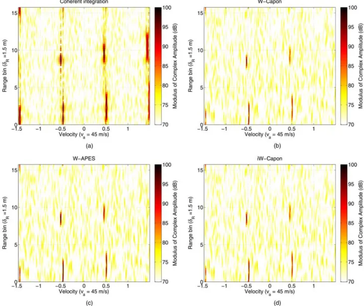
3) Range-Velocity Maps: The range-Doppler maps are depicted in Fig. 7 for the coherent integration, the W-Capon, the W-APES, and the iW-Capon algorithms. The processing parameters are the same as those described in Table III except for the unfolding factor that is set to nva= 3. The number of iterations is set to 3 for the iW-Capon procedure. The following remarks can be made accordingly.
Clutter filtering. From the maps in Fig. 7, it appears that most clutter components have been removed by the ad-hoc filter (Fig. 6). Although, few residues seem to remain, especially around the range bin 6 (see Fig. 7(d)). Note that the proposed filter has certainly removed not only the ground clutter but also some slow targets as well as targets in blind velocities.
Velocity dealiasing. Trends observed with synthetic data are recovered here. The sidelobes observed for a coherent integration algorithm greatly pollute the range-velocity maps. The maps become cleaner and cleaner with W-Capon, W-APES, and iW-Capon. Note that, contrary to narrowband techniques, the wideband estimators of interest here can determine the true target velocity from one burst with a single low PRF.
Possible observed scenario. We believe that the iW-Capon algorithm is the most reliable processing in the sparse-target environment, and we, thus, infer from it (via Fig. 7(d)) the following possible target
Fig. 7. Comparison of spectral estimates. PARSAX experimental data. (a) Coherent integration. (b) W-Capon. (c) W-APES. (d) iW-Capon. scenario j®1j2= 102 dB, v1=¡24 m/s, `0,1= 8:75 (51a) j®2j2= 99:8 dB, v2=¡21:6 m/s, `0,2= 2:25 (51b) j®3j 2= 99:6 dB, v 3=¡21:7 m/s, `0,3= 0:75: (51c) Note that the received signals have not been
normalized after the fast Fourier transform (FFT) operation performed during the deramping processing, which explains the high amplitude level.
4) Range-Velocity Maps for Quasi-Equivalent Synthetic Scenario: To validate our interpretation (51) of the experimental scenario, a quasi-equivalent synthetic data exempt from clutter has been
reconstructed according to (21). Also, the thermal noise level has been approximately set such that SNR1¼ 0 dB. The range-velocity maps obtained with this synthetic scenario are depicted in Fig. 8. The maps are very similar to those obtained with the experimental data. Moreover, as there are no clutter residues, the reconstructed maps are “cleaner.” The advantage of the iW-Capon estimator compared with the W-Capon estimator is more obvious with the experimental data. It is of interest to note that the level of main and sidelobe peaks are recovered for the two close-range targets, i.e., t = 2 and t = 3. However, the sidelobe levels of the brightest target t = 1 are much higher with the experimental data than with the synthetic scenario. For instance, it can be clearly seen from Figs. 7(d) and 8(d) that with the experimental data a sidelobe is observed at v1+ 2va, while it does not even appear for synthetic data. A
Fig. 8. Comparison of spectral estimates. PARSAX synthetic data. (a) Coherent integration. (b) W-Capon. (c) W-APES. (d) iW-Capon.
possible explanation is that the brightest target may be, in fact, the result of several close-range scatterers. This observation opens a challenging question that will be investigated in future work: what is the range-velocity resolution of our proposed wideband spectral estimators?
VI. CONCLUSION
Wideband radar is a key concept for designing future radar systems as it may provide high
performance for detection of small targets in hostile environments. In this paper we have focused our attention mostly on the problem of the range migration that occurs for fast moving targets. More specifically, we have presented an adequate wideband signal model for pulse waveform that takes into account linear migration. Accordingly, we have proposed and studied the performance of three new spectral estimators: W-APES, W-Capon, and iW-Capon. These estimators outperform the
narrowband estimators as well as a simple coherent summation. Indeed, they take advantage of the range migration, thereby mitigating velocity sidelobes and providing an enhanced discrimination between migrating point-targets. The performance of W-APES, W-Capon, and iW-Capon has been assessed on synthetic and experimental data collected from the PARSAX system. Wideband spectral estimators have been applied on experimental data after a preprocessing step for clutter filtering. Future work includes the refinement of the preprocessing filtering as well as a thorough study on the range-velocity resolution of the proposed wideband estimators. APPENDIX
It is shown in this Appendix that problem (36) does not have a priori a closed-form expression.
In order to derive ˆ®wapes(36), the log-likelihood