Modeling Approach for the Prediction of Transient and Permanent Degradations of Image Sensors in Complex Radiation Environments

Any correspondence concerning this service should be sent to the repository administrator:

staff-oatao@inp-toulouse.fr

O

pen

A

rchive

T

oulouse

A

rchive

O

uverte (

OATAO

)

OATAO is an open acce

ss repository that collects the work of Toulouse researchers

and makes it freely available over the web where possible.

This is an author -deposited version published in:

http://oatao.univ-toulouse.fr/

Eprints ID: 11033

To link to this article:

DOI:10.1109/TNS.2013.2284798

URL:

To cite this version: Raine, Mélanie and Goiffon, Vincent and Girard, Sylvain and Rousseau,

Adrien and Gaillardin, Marc and Paillet, Philippe and Duhamel, Olivier and Virmontois, Cédric

Modeling Approach for the Prediction of Transient and Permanent Degradations of Image

Sensors in Complex Radiation Environments. (2013) IEEE Transactions on Nuclear Science,

vol. 60 (n° 6). pp. 4297-4304. ISSN 0018-9499

Abstract— A modeling approach is proposed to predict the transient and permanent degradation of image sensors in complex radiation environments. The example of the OMEGA facility is used throughout the paper. A first Geant4 simulation allows the modeling of the radiation environment (particles, energies, timing) at various locations in the facility. The image sensor degradation is then calculated for this particular environment. The permanent degradation, i.e. dark current increase, is first calculated using an analytical model from the literature. Additional experimental validations of this model are also presented. The transient degradation, i.e. distribution of perturbed pixels, is finally simulated with Geant4 and validated in comparison with experimental data.

Index Terms— Active Pixel Sensor (APS), CMOS Image Sensor (CIS), dark current distribution, Single-Event Transient (SET), Displacement Damage Dose (DDD), Inertial Confinement Fusion (ICF), Geant4, neutrons.

I. INTRODUCTION

HEN operating in radiation environments, image sensors may suffer a variety of degrading effects, such as dark current increase and Single Event Transient (SET)-induced saturated pixels, either due to ionizing effects, non-ionizing effects or a combination of both, depending on the nature of radiations they are submitted to ([1], [2]). Because of these multiple possible degradations, the effect of mixed environments is particularly complex to model, since for example protons themselves will induce Single Event, Total Ionizing Dose (TID) and Displacement Damage Dose (DDD) effects. The equation is even more complex for environments combining different kinds of particles.

New complex radiation environments emerge today for scientific applications, including running facilities such as the National Ignition Facility (NIF) [3] or the Large Hadron Collider (LHC) ([4], [5]), in construction ones such as the Laser Megajoule (LMJ) [6] or the International Thermonuclear M. Raine, A. Rousseau, M. Gaillardin, P. Paillet and O. Duhamel are with CEA, DAM, DIF, F-91297 Arpajon, France (e-mail : melanie.raine@cea.fr).

V. Goiffon is with ISAE, Université de Toulouse, 10 av. E. Belin, F-31055 Toulouse, France.

S. Girard is with Laboratoire Hubert Curien – UMR CNRS 5516, 18 rue du Pr. Benoît Lauras, F-42000 Saint Etienne, France.

C. Virmontois is with CNES, F-31401 Toulouse, France.

Experimental Reactor (ITER) [7], and future projects, such as the High Power laser Energy Research (HiPER) [8], the Laser Inertial Fusion Energy (LIFE) [9] and the Super LHC. Other needs also include instrumentation for space applications, or those appearing more recently, such as surveillance missions in nuclear power plants, due to additional security constraints following the Fukushima Daichii event. Image sensors are or will be used in all these facilities, from security systems to diagnosis applications.

In such facilities, the replacement of devices may be complex, sometimes even not possible; dedicated tools are then needed to predict their lifetime and the degradation of their performances for a given application [10]. This paper describes the approach followed for LMJ, which represents a case study combining different kinds of particles (X-rays,

γ−rays and 14 MeV neutrons), transient and permanent effects.

A detailed description discussing this specific harsh environment can be found in reference [11]. This paper intends to be a proof of concept for a methodology that can then be

extrapolated to other radiation environments.

First, a general description of the proposed modeling approach is given. The details of the different steps are described in the following sections, giving also justifications regarding the chosen tools. When available, experimental verification of the simulated/calculated results is performed.

II. MODELING APPROACH

This section describes the general concept of the modeling approach developed to predict transient and permanent degradations of image sensors in complex radiation environments, with a particular focus on the one for LMJ.

During a laser shot, up to 5x1018 neutrons will be produced in

a very short period of time (100 ps), in a localized region of approximately 60 µm. These neutrons will then propagate in the 30 m-diameter experimental hall, interacting with the different present volumes and finally reach the different image sensors we are interested in. Given the orders of magnitude of the dimensions and fluences involved, a complete direct calculation of the radiation effect at the device level does not seem feasible.

Modeling Approach for the Prediction of

Transient and Permanent Degradations of Image

Sensors in Complex Radiation Environments

Mélanie Raine, Member, IEEE, Vincent Goiffon, Sylvain Girard, Senior Member, IEEE,

Adrien Rousseau, Marc Gaillardin, Member, IEEE, Philippe Paillet, Senior Member, IEEE,

Olivier Duhamel, Cédric Virmontois, Member, IEEE

Fluence = f(E)

@location, time…

Simulation of radiation environment (particles, energy, hit time…) at given location in complex geometry

n

γ

Geant4 simulation

DDD

DDD calculation

…

Geant4 simulation

Analytical model

f(

_∆

I

)

Ionizing

Edep

in pixel

Size: meters

Size: µm

ENVIRONMENT

RADIATIVE EFFECTS

Dose

SET

f(

_∆

I

)

Fluence = f(E)

@location, time…

Simulation of radiation environment (particles, energy, hit time…) at given location in complex geometry

n

γ

Geant4 simulation

DDD

DDD calculation

…

Geant4 simulation

Analytical model

f(

_∆

I

)

Ionizing

Edep

in pixel

Size: meters

Size: µm

ENVIRONMENT

RADIATIVE EFFECTS

Dose

SET

f(

_∆

I

)

Fluence = f(E)

@location, time…

Simulation of radiation environment (particles, energy, hit time…) at given location in complex geometry

n

n

γ

γ

Geant4 simulation

DDD

DDD calculation

…

Geant4 simulation

Analytical model

f(

_∆

I

)

Ionizing

Edep

in pixel

Size: meters

Size: µm

ENVIRONMENT

RADIATIVE EFFECTS

Dose

SET

f(

_∆

I

)

Fig. 1: Schematic representation of the proposed modeling approach to determine permanent and transient degradation of image sensors in complex radiation environments.

It would require simulating both the global geometry involving dimensions in the order of tens or hundreds of meters, and the sensor itself, with pixels of a few micrometers. This raises technical issues among which the involved computational time is not the least. That is why we choose to split the calculation in different steps. Figure 1 is a graphic representation of the chaining of these steps. Their detailed description and application to concrete cases are developed in following sections.

The first step towards the prediction of transient and permanent degradations of image sensors is to determine the radiation environment they are submitted to. For the case study of the LMJ, the main challenge lies in the complexity of the geometry to consider. The goal is to determine the energy and temporal spectra of the radiation environment at the device location – or to determine the best location for the device depending on its function, the determined environment and the amount of radiation it can withstand. To do so, Monte Carlo particle-matter interaction simulation codes such as Tripoli ([11], [12]) or Geant4 ([13], [14], [15]) are well suited.

Once the radiation background is well described, the second step is to determine its effect on the device. This step is realized several times, for each component of the nuclear environment, to discriminate the contribution of each kind of particle. Moreover, it is divided in two categories: permanent (or dose) effects and transient effects (called Single-Event Transients or SET hereafter).

Permanent effects are also divided in two parts, with the Total Ionizing Dose (TID) on one hand and the Displacement Damage Dose (DDD) on the other. In this paper, we will focus on DDD, since permanent ionization effects in image sensors are expected to be negligible in the LMJ environment. DDD induces large Dark Current Non Uniformity (DCNU), with dark current distributions exhibiting hot pixel tails after irradiation. Various models have been proposed to calculate these dark current increase distributions ([16], [17], [18], [19]). In this paper, we choose to use one of the most recent ones [20]; it presents several advantages but still requires additional validation, as detailed in the dedicated section.

Regarding transient effects, the neutron radiation pulse randomly generates signal charges in the pixel array through indirect localized ionization. The result can be represented as a distribution of charges deposited by the radiation pulse in the pixel array and collected by the pixel photodiodes. We propose to approximate this response by simulating the distribution of deposited energy in the pixel array using a second Geant4 simulation.

III. RADIATION ENVIRONMENT DETERMINATION

The first step corresponds to the simulation of the radiation environment at a given location in the complex geometry. It involves geometries in the order of tens or hundreds of meters. While the ultimate goal is to predict the behavior of image sensors in the LMJ environment, no data are by definition

3 0 2 4 6 8 10 12 14 10-3 10-2 10-1 100 101 102 103 104 @ 50 cm @ 5 m F lu e n c e ( n /c m 2 ) Energy (MeV)

108 incident 14 MeV neutrons

Geometrical 14 MeV fluence

Fig. 2: Geant4 simulated neutron spectra at two different locations in the OMEGA experimental hall.

available for this configuration. However, recent work aiming at investigating the vulnerability of CMOS Active Pixel Sensors (APS) in Megajoule class laser environments presented results of experiments at the OMEGA facility in Rochester, NY, USA ([21], [22]). This facility provides a unique platform to evaluate the effects of a pulsed mixed radiation environment, at a neutron yield lower than the one

expected for LMJ (1013 instead of 1018 neutrons per shot) but

representative of preliminary Inertial Confinement Fusion (ICF) experiments in megajoule class laser facility. At first, we thus choose to simulate the geometry of the OMEGA facility, to be able to use the calculated spectrum in following steps and compare the results to available experimental data.

This geometry is simulated using the Monte Carlo Geant4 simulation toolkit version 9.4. It includes the 80 m long experimental hall walls, the 3 m-diameter inner aluminum sphere and all significant volumes around it, as illustrated in the first step in Fig. 1. All materials with concentration higher than 1% are taken into account; materials which neutron interaction cross-sections are known to be particularly high

(10B for example) are also included whatever their

concentration. The G4NeutronHP physics list is used; since the focus of the simulation is on neutron fluences, all generated charged particles are ignored to limit calculation

time. A total number of 108 simulated 14 MeV neutrons are

emitted isotropically from a point source located at the center of the target chamber. This number allows getting good

statistics while limiting the calculation time (High

Performance Computing resources were still required for this simulation [23]). The resulting environment (particle, energy, hit time) is recorded with perfect detectors at two different distances from the TCC (Target Chamber Center), corresponding to different sets of available data: 50 cm (inside the target chamber) and 5 m (outside the target chamber). As stated earlier, the image sensor itself is too small for the simulation time to be efficient if the detectors were limited to micrometer-size pixels. The detectors are thus represented by

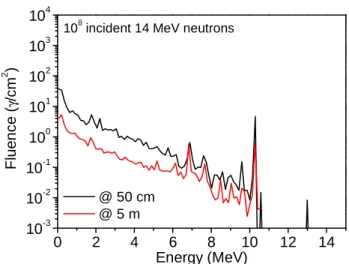
0 2 4 6 8 10 12 14 10-3 10-2 10-1 100 101 102 103 104 F lu e n c e ( γ /c m 2 ) Energy (MeV) @ 50 cm @ 5 m

108 incident 14 MeV neutrons

Fig. 3: Geant4 simulated gamma spectra at two different locations in the OMEGA experimental hall.

1 mm-thick sphere portions, several cm2 large. This allows

limiting the number of incident particles needed to get sufficient statistics, while having limited impact on resulting spectra, given the involved dimensions.

The simulated neutron spectra, integrated over 100 ms, obtained at both locations are displayed in Fig. 2. The star-shaped symbols represent the theoretical calculations of 14 MeV neutrons fluence at these locations from simple geometrical principles, when no interaction is taken into account. This calculation is a first confirmation of the consistency of the simulation: the proportion of 14 MeV neutrons in simulated spectrum is below this theoretical value in both cases and a lower number of 14 MeV neutrons remain at a distance of 5 m than at 50 cm from the center of the target chamber.

While interacting in the experimental hall, neutrons also generate other particles. Charged particles are not considered here for simulation time reasons and because they will stop close to their generation location after ionization interactions (for example, the range of 14 MeV protons in aluminium is of only 1.1 mm). On the contrary, the generated gamma rays will be able to propagate throughout the experimental hall and maybe affect the image sensors studied in this paper. The corresponding spectra are thus extracted from simulation and reported in Fig. 3 for both locations.

It may be noted that this stage of the approach may also be used to evaluate the feasibility of a hardening-by-system study through shielding of the image sensor for example. The temporal aspect (not detailed here) can also be exploited and lead to mitigation techniques ([22], [24]).

IV. PERMANENT RADIATION EFFECTS

In the second step, the goal is to predict permanent radiation effects induced by DDD in image sensors, in order to estimate the lifetime of the image sensor in the facility depending on its location and profile of use. To do so, we choose to rely on the model described in [20], which appears quite simple to

4 10-2 10-1 100 101 102 103 104 10-5 10-4 10-3 10-2 N IE L ( M e V. c m 2 /g ) Energy (MeV)

Fig. 3: NIEL variation in silicon versus incident neutron energy, from [25]. implement, involves no fitting on experimental data and has been shown to fairly well predict the dark current increase distribution, based only on a few parameters: the depleted

volume Vdep of the considered image sensor, the DDD and two

fixed factors named υdark and γdark . The dark current increase

distribution is then calculated from the following equations:

{ }

(

)

x

Poisson

N

f

I

f

=

∑

×

∆

,

)

(

µ

{ }

!

)

exp(

,

N

N

Poisson

µ

µ

µ

=

×

−

DDD

V

×

×

=

γ

µ

1

(

)

∫

∗

∗

=

t

f

x

f

f

x

f

)

(

)

(

...

)

(

(

)

_











₋

_∆

×

=

∆

I

I

f

υ

υ

exp

1

According to the analysis performed in [20], the factors υdark

and 1/γdark can be attributed to the mean dark current increase

induced by a Single Particle Displacement Damage Effect (SPDDE) and to the SPDDE probability normalized to the volume and dose respectively. A SPDDE corresponds to the cascade of displacements that may be induced by a single incident particle (a neutron here) in a pixel volume; some of these displacements will then result in electro-active Shockley-Read-Hall generation centers.

To use this model in the following, the first step is to calculate the DDD at a specific location for a given incident fluence. To do so, the variation of the NIEL (Non-Ionizing Energy Loss) with incident neutron energy, represented in Fig. 3 (from reference [25]) is used to correlate each element of the energy spectrum with a NIEL value.

Some points then remain to be validated to apply the model to our study. First, the influence of annealing and measurement

temperature on the two parameters υdark and γdark of the model

has not been discussed in [20]. Second, this model has only been validated with mono-energetic beams. While it seems to depend only on the total received DDD, it is worth demonstrating that consistent results are obtained even following irradiation with an incident energy spectrum. Third, in the case of the LMJ, the model will be applied to a dose received in a succession of different shots, separated by an unavoidable annealing period. It would thus be interesting to confirm that the same dose received from a single irradiation or after multiple shots separated in time will result in the same degradation on the device (considering sufficient annealing time after the end of the last irradiation).

To demonstrate these different points, different irradiations are performed. The studied CMOS image sensors are manufactured in a 0.18-µm commercial process. They are 10 µm-pitch 128x128 pixel arrays with 3T-pixels using conventional photodiodes and are processed in a 7 µm silicon epitaxial layer. They are exposed to neutron beams at CEA, France and UCL, Belgium.

A. Influence of annealing time

In [20], all measurements were made at 23°C and an average annealing time of 3 weeks was considered. The values

of the two factors υdark and γdark of the model are thus given for

these particular testing conditions. However, similarly to the

Universal Damage Factor (UDF) κdark corresponding to the

mean dark current increase normalized to the volume and dose introduced by Srour in [26], these two parameters actually depend on the measurement temperature and on the annealing time after irradiation. While the measurement temperature can be easily controlled and fixed to 23°C, it is not always possible to get the devices back 3 weeks after irradiation to measure the dark current increase. The data were thus analyzed carefully to take this time into account in the two factors. Following this

analysis, their values are then fixed at υdark = 0.81 fA (or

5070 e-/s) and γdark = 4.0 x 104 µm3.TeV/g for 23°C and 3

weeks of annealing. It is remarkable to note that using these

values, the ratio υdark/γdark equals the UDF κdark at the same

temperature and annealing time. This seems logical,

considering that υdark represents the mean dark current increase

due to a SPDDE, 1/γdark is the SPDDE probability normalized

to the volume and dose and κdark = υdark/γdark is the mean dark

current increase normalized to the volume and dose.

Following this observation, the parameters υdark and 1/γdark

are extrapolated to take into account the annealing time using the annealing factor introduced by Srour in [26] for the UDF. This method is applied on different sets of experimental data measured after different annealing time. The results are reported in Fig. 4, for two different irradiations, at different energies and different DDD. Here and in the following, “normalized number of pixels” means that the integral of the distribution is equal to one. Along with experimental data, the calculations obtained with the model from [20] are reported as solid lines, with annealing corrections. These data show that

5 0 2 4 6 8 10 10-3 10-2 10-1 100

Model w/o correction

(υ and γ @ 3 weeks)

Model w/ anneal. correction

N o rm a liz e d n u m b e r o f p ix e ls

Idark increase (fA)

20 MeV, 670 TeV/g, 4 wks 6 MeV, 400 TeV/g, 7 wks

Fig. 4: Dark current distribution in 128x128 pixels CIS measured after exposition to neutrons for two different energies, DDD and annealing times. The lines are the result from calculation using the model described in [20].

TABLE I:NEUTRON RRADIATION DETAILS: ENERGY, FLUENCE AND DOSE

the corrected model is in very good agreement with experimental data, whatever the energy, dose and annealing time. The calculations issued from the model without any corrections, using the two parameters determined previously, are also reported as dotted lines, showing the increasing importance of taking into account the annealing time in the calculations with increasing time compared to the 3 weeks reference.

For future work, it would be interesting to explore in details

the physical meaning of the two parameters υdark and γdark,

through experiments or calculations. This would allow really fixing the values of these (for now) empirical parameters. A dedicated study should also be performed to see if the

evolution of κdark with temperature can be extrapolated for υdark

and 1/γdark as is done here for annealing.

B. Spectrum vs. monoenergetic irradiation

The next point is to validate the use of this analytical model for irradiations with incident energy spectrum instead of mono-energetic beams. To do so, energy spectrum are “re-created” by exposing the same device successively at different energies: namely 3.5, 4 and 6 MeV, for a total DDD of 400 TeV/g for one device and 15.5, 16, 18 and 20 MeV for a total DDD of 540 TeV/g for a second device. For comparison

0 2 4 6 8 10 10-3 10-2 10-1 100 N o rl m a liz e d n u m b e r o f p ix e ls

Idark increase (fA)

Cumulated energy Mono-energy 6 MeV Virmontois' model

n, 400 TeV/g 23°C, 7 weeks

Fig. 5: Dark current distribution in 128x128 pixels CIS measured after exposition to neutrons for a DDD of 400 TeV/g, applied either with a “reconstructed spectrum” combining 3.5, 4 and 6 MeV neutrons beams (red circles) or with a mono-energetic 6 MeV neutron beam (black squares). The blue line is the result from calculation using the model described in [20].

0 2 4 6 8 10 10-3 10-2 10-1 100 N o rm a liz e d n u m b e r o f p ix e ls

Idark increase (fA)

Cumulated energy: 15.5, 16, 18 and 20 MeV

Virmontois' model

n, 540 TeV/g 23°C, 4 weeks

Fig. 6: Dark current distribution in 128x128 pixels CIS measured after exposition to neutrons for a DDD of 540 TeV/g, applied with a “reconstructed spectrum” combining 15.5, 16, 18 and 20 MeV neutrons beams (black squares). The blue line is the result from calculation using the model described in [20].

with the first “spectrum”, a third device is exposed to the same total DDD of 400 TeV/g, but using only the mono-energetic 6 MeV beam. The details of the fluence used at each energy are reported in Table I for all three irradiations. The results in terms of dark current increase distribution are reported in Fig. 5 and 6 respectively for the two DDD values, along with the result from calculations using the model from [20]. In both figures, all sets of data are in very good agreement, thus giving a first confirmation of the validity of the model for irradiations with an energy spectrum.

The calculation is then performed for the OMEGA spectrum at 50 cm from the center of the target chamber, for which experimental data are available in [21]. The dark current measurements are reported in red in Fig. 7, along with the result from our calculation based on the energy spectrum represented in Fig. 2. The experimental data correspond to raw Device Energy (MeV) Fluence (n/cm²) DDD (TeV/g) Total DDD (TeV/g) Fig. 1 3.5 4.1x1010 100 400 Fig. 5 4 3.8x1010 110 6 5.9x1010 190 2 6 1.5x1011 400 400 Fig. 5 3 15.5 4.7x1010 195 540 Fig. 6 16 2.2x1010 90 18 3.8x1010 145 20 2.9x1010 110

6 0.0 0.5 1.0 1.5 2.0 2.5 3.0 3.5 0.01 0.1 1 10 P ix e l fr e q u e n c y ( A .U )

Dark current (fA) Exp. data

Calculation (spectrum)

Fig. 7: Dark current distribution of 128x128 pixels CIS measured after exposition to neutrons at 1010 n/cm² fluence in OMEGA at 50 cm from the center of the target chamber (data from [21]). Calculations of the dark current increase based on Geant4 simulated OMEGA spectrum @50cm from Fig. 2.

0 10 20 30 40 50 0.00 0.05 0.10 0.15 0.20 0.25 0.30 0.35 A b s o lu te f lu x ( 1 0 1 1 n /s /s r) Energy (MeV)

Fig. 8: Energy spectrum of the high flux neutron beam at UCL [27], [28]. dark current values, the initial Gaussian-shape distribution (below 0.5 fA) representing pixels which are not impacted by the irradiation. Since the calculation gives dark current

increase values, the calculated distribution is shifted to ignore

this Gaussian distribution. The resulting “spectrum”

calculation is in good agreement with experimental data. As expected, the calculated TID induced by the gamma spectrum

presented in Fig. 3 is negligible (~1x10-4 rad) and has no

impact on the dark current distribution. However, this means

that a 1018 neutrons LMJ shot would induce a TID of ~1 krad

(at 50 cm) that may need to be taken into account.

Finally, an irradiation is performed with the high flux neutron beam from UCL ([27], [28]). The energy spectrum, from 5 to 50 MeV neutrons, is reported in Fig. 8. The result

from irradiation at a fluence of 1011 n/cm2, corresponding to a

DDD of 400 TeV/g, and after 2 weeks of annealing is reported in Fig. 9, along with calculations from the model. Again, both sets of data are in very good agreement. This gives a final validation that the model only depends on the DDD and not on the incident energy spectrum. Additionally, it also shows again

0 2 4 6 8 10 10-3 10-2 10-1 100 No rm a liz e d n u m b e r o f p ix e ls

Idark increase (fA)

UCL spectrum Model

n, 400 TeV/g 23°C, 2 weeks

Fig. 9: Dark current distribution in 128x128 pixels CIS measured after exposure to the high flux neutron beam at UCL, for a DDD of 400 TeV/g, after 2 weeks of annealing. The blue line is the result from calculation using the model described in [20].

the good adaptation of the model taking into account the annealing time.

C. Multiple shots vs. single irradiation

It was not possible to properly address the question of the applicability of the model to a dose received after multiple shots for this paper. However, the results presented in Fig. 5 and 6 for irradiations of single devices with multiple energies give first insights: these irradiations were indeed performed in several days, typically spread over a week, with annealing times at ambient temperatures between irradiations. Given the good agreement with monoenergetic irradiations performed in one time in Fig. 5 and with the model from [20] for both sets of data, these particular irradiation conditions do not seem to affect the final result.

V. TRANSIENT RADIATION EFFECTS

The second “radiation effect” step deals with Single-Event Transients in pixels during irradiation. This calculation is particularly important for LMJ, to identify the limit of use or the lifetime of the image sensor depending on the intensity of foreseen shots. For this step, a second Geant4 simulation is performed. To validate the simulation, measurements of the transient response of an APS during a laser shot performed at the OMEGA facility [21] are used. The measured sensor is a 13 µm-pitch 1024x1024 pixel array with 3T-pixels using conventional photodiodes, manufactured using a 0.35 µm CMOS process. The substrate is a slightly P-doped epitaxial layer approximately 8 µm thick grown on top of a heavily P-doped 300 µm-thick substrate [29].

At first, the geometry is reduced to a 13x13x308 µm3 silicon

box topped by 10 µm SiO2 overlayers, representative of a

single image sensor pixel. The physics list is the same as in the previous Geant4 simulation, except that this time, tracking of charged particles is included; they will indeed be responsible for SETs. The energy of incident neutrons is distributed following the previously calculated energy spectrum. The total

7 0 50 100 150 100 101 102 103 104 105 106 P ix e l c o u n t Signal (ke-) Exp.

Simul. single pixel Simul. 1024x1024

> 140 ke

-7x106 n/cm2

Fig. 10: Experimental [21] and simulated distribution of the number of generated electrons after irradiation in OMEGA at 5 m from the center of the target chamber.

deposited energy is recorded for each incident particle, in the epitaxial layer of the simulated pixel. To limit the amount of registered data, only non-zero values are recorded.

Measurements of the transient response of an APS during a laser shot performed at the OMEGA facility from [21] are reported in Fig. 10, showing the number of pixels suffering a given perturbation (the signal is expressed as a number of

generated electrons). This figure corresponds to a

“geometrical” fluence of 7x106 n/cm2 at 5 m. The

corresponding “real” number of neutrons striking the device is calculated from the previously calculated spectrum (Fig. 2) and used in the simulation. Simulations were also performed for the incident gamma spectrum, but the resulting deposited energy values are quite small, only contributing in the first three to four first bins of the histograms in Fig. 10. This contribution is not considered significant and is thus ignored in the following. In Fig. 10 simulation results (squares), the last

symbol “> 140 ke-” represents simulated values higher than

140 ke-, which are not measured experimentally because of the

pixels saturation [21]. These points actually correspond to the experimental Gaussian distribution that appears above

~125 ke-. This population of saturated pixels does not appear

as a single distribution mainly because of the disparity in saturation levels between different pixels.

The first simulation results taking into account a single pixel are reported as empty squares. While the general shape of the curve is in good qualitative agreement with experimental data, the simulated distribution is clearly below the experimental one. The opposite was expected since only the deposited energy is simulated, not taking into account recombination or collection efficiency mechanisms (no charge amplification is expected here).

To improve the simulated distribution, simulations are then performed taking into account an array of pixels. The result for a 1024x1024 array (corresponding to the tested device) is reported as black squares in Fig. 10. This time, the simulated curve is above the experimental one, as expected. However,

0 100 200 1024 3000 4000 5000 100x100: 1h30 1024x1024: 36h N u m b e r o f e v e n ts Number of pixels (NxN)

Single pixel: 23 min.

Fig. 11: Number of non-empty events recorded in the simulation depending on the number N of pixels in the NxN array.

this simulation taking into account the complete geometry is quite long (36 h). Different sizes of pixel arrays are thus tested, to find a good compromise between size, time and quality of the result. In Fig. 11 are reported the results as the number of non-empty events depending on the simulated device size for 1x1, 3x3, 6x6, 10x10, 100x100 and 1024x1024 pixel arrays. Some simulation times are also reported as reference. While the number of non-empty events keeps increasing with the number of pixels in the array, the difference from 100x100 to 1024x1024 is much less important than earlier in the curve, while the difference in simulation time is important, from 1h30 to 36h. Consequently, the 100x100 pixel array seems to be a good compromise; this size is used in the following. The resulting event distribution is very similar to the 1024x1024 one represented in Fig. 10. This continuous increase of events with the size of the matrix was not necessarily expected; when dealing with border crossing effects, the used metric is usually the largest range of secondary heavy ions, i.e. a few micrometers, meaning that the geometry should be extended only to the few neighboring pixels. The continuous increase observed here probably means that among the generated secondary protons or neutrons, some are able to travel in the matrix and interact much further than the closest neighbors of their initial generation pixel. Ignoring these far-traveling secondaries result in the underestimation of the experimental distribution shown for example in Fig. 10 with the “single pixel” simulation. Similarly, taking into account the full vertical stack of material is important to generate all events able to reach the epitaxial layer of one pixel.

To further validate the simulation, the number of saturated and disturbed-only pixels is also explored. As defined in [21], pixels are considered as disturbed if they exhibit values above 15 ke- and as saturated above 125 ke-. In the following, “disturbed” corresponds to pixels which are disturbed but not saturated, i.e. with values between 15 and 125 ke-. The comparison of this repartition of pixels is done for the 3 different fluences whose distributions are presented in [21]:

8 1x106 3x106 5x106 7x106 0 500 1000 1500 2000 Disturbed pixels N u m b e r o f p ix e ls Geometrical fluence (n/cm2) Exp. Simul. 100% efficiency Simul. 40% efficiency Saturated pixels

Fig. 12: Number of disturbed-only and saturated pixels as a function of the incident geometrical neutron fluence, extracted from experimental data and simulation results, either taking into account 100% or 40% collection efficiency.

1.8x106, 3x106 and 7x106 n/cm2. As before, these values

correspond to geometrical calculations; the “real” numbers of neutrons distributed in the energy spectrum are used in the simulations. Disturbed and saturated numbers of pixels extracted from both experimental and simulation results are reported in Fig. 12, in black squares and red circles respectively. This analysis confirms the observation made in Fig. 10 showing that the simulated number is always higher than experimental values, both for disturbed and saturated pixels. A correcting “collection efficiency” factor is thus applied to simulation results to take into account the various mechanisms leading to a collected charge lower than the generated one. To adjust the simulation value to the

experimental number of saturated pixels at 7x106 n/cm2, a

collection efficiency of 40% is determined. Such efficiency is not unusual in image sensors [30]. The simulation results corrected with this collection efficiency factor are reported in Fig. 12 as blue empty circles and dotted lines, for disturbed and saturated pixels and for all fluences. These corrected results are in very good agreement with experiments for all cases.

In the case of predictive calculations, this efficiency factor will however probably not be known. Yet, this is not a big issue since raw results from simulation with 100% efficiency actually give a worst-case scenario. In the example of Fig. 12, the number of disturbed pixels would be overestimated by not more than 50% and the number of saturated pixels by a factor of less than 3. A satisfying analysis of vulnerability can probably be performed even using these overestimated values.

VI. CONCLUSION

This paper intends to be a proof of concept for a methodology to predict the degradation of image sensors in a given complex radiation environment. The case study of LMJ is chosen but the method can then be extrapolated to other radiation environments. This paper gives a description of the method, decomposed in different steps. The radiation

environment is first simulated at specific locations in a large facility (the example of the OMEGA facility is used here). The permanent degradation is then calculated using an analytical model of the literature. For the purpose of the application studied here, this model is also further extended and validated: the annealing time after irradiation is now taken into account; experimental data are used to validate the applicability of the

model for multi-energy and multi-shots irradiations,

reinforcing the fact that it only depends on the final DDD. Finally, the transient degradation of the image sensor during irradiation is simulated with Geant4, and compared to experimental data, with very satisfying results.

To further extend the model and make it universally applicable to any radiation environment, TID effects would also need to be taken into account. These ionizing dose effects result in a uniform increase of the dark current (as opposed to the distribution of dark current increase induced by DDD), which, at first order, translates the initial Gaussian distribution towards larger dark current values. An attempted model of this uniform increase has been presented in [31]. However, this model was developed from fitting to experimental data and some parameters most certainly depend on the studied device geometry and characteristics. A more complete study analyzing large sets of data would be needed to assess the potential of developing a universal model such as the one used here for DDD. Moreover, the combination of a TID model with the DDD model presented in this paper is not necessarily straightforward, as shown in [20]. A dedicated study is thus required to be able to add the TID modeling block to the methodology presented in this paper. This will be the subject of future work.

ACKNOWLEDGEMENTS

The authors would like to thank the Van der Graaf team at CEA/DAM/DIF, France, F. Jacquot and the team at CEA/Valduc, France and N. Postiau and the team at UCL, Belgium for their support to access and perform neutron irradiations.

REFERENCES

[1] G. R. Hopkinson, "Radiation effects in a CMOS active pixel sensor", IEEE Transactions on Nuclear Science, vol. 47, pp. 2480 - 2484, 2000.

[2] J. R. Srour, C. J. Marshall and P. W. Marshall, "Review of displacement damage effects in silicon devices", IEEE Transactions on Nuclear Science, vol. 50, pp. 653 - 670, 2003. [3] NIF [Online]. Available: https://lasers.llnl.gov

[4] LHC [Online]. Available: http://lhc.web.cern.ch

[5] A. I. Drozhdin, M. Huhtinen and N. V. Mokhov, "Accelerator related background in the CMS detector at LHC", Nuclear Instruments and Methods in Physics Research A, vol. 381, pp. 531 - 544, 1996.

[6] LMJ [Online]. Available: http://www-lmj.cea.fr [7] ITER [Online]. Available: http://www.iter.org [8] HiPER [Online]. Available: www.hiper-laser.org [9] LIFE [Online]. Available: https://life.llnl.gov

[10] J.-L. Bourgade, et al., "Present LMJ diagnostics developments integrating its harsh environment", Review of Scientific Instruments, vol. 795, pp. 10, 2008.

9 [11] J.-L. Bourgade, et al., "New constraints for plasma diagnostics

development due to the harsh environment of MJ class lasers", Review of Scientific Instruments, vol. 75, pp. 4204 - 4212, 2004. [12] H. P. Jacquet, L. Lachèvre and M. Messaoudi, "Activation

analysis and first occupational dose rates estimates for the Laser Megajoule facility", Radiation Protection Dosimetry, vol. 116, pp. 290 - 292, 2005.

[13] Geant4 [Online]. Available: http://geant4.web.cern.ch/geant4 [14] S. Agostinelli, et al., "GEANT4 - A simulation toolkit", Nuclear

Instruments and Methods in Physics Research A, vol. 506, pp. 250 - 303, 2003.

[15] J. Allison, et al., "Geant4 develoments and applications", IEEE Transactions on Nuclear Science, vol. 53, pp. 270 - 278, 2006. [16] P. W. Marshall, C. J. Dale, E. A. Burke, G. P. Summers and G. E.

Bender, "Displacement damage extremes in silicon depletion regions", IEEE Transactions on Nuclear Science, vol. 36, pp. 1831 - 1839, 1989.

[17] C. J. Dale, P. W. Marshall and E. A. Burke, "Particle-induced spatial dark current fluctuations in focal plane arrays", IEEE Transactions on Nuclear Science, vol. 37, pp. 1784 - 1791, 1990. [18] P. W. Marshall, C. J. Dale and E. A. Burke, "Proton-induced

displacement damage distributions and extremes in silicon microvolumes", IEEE Transactions on Nuclear Science, vol. 37, pp. 1776 - 1783, 1990.

[19] C. J. Dale, L. Chen, P. J. McNulty, P. W. Marshall and E. A. Burke, "A comparison of Monte Carlo and analytic treatments of displacement damage in Si microvolumes", IEEE Transactions on Nuclear Science, vol. 41, pp. 1974 - 1983, 1994.

[20] C. Virmontois, V. Goiffon, P. Magnan, S. Girard, O. Saint-Pé, S. Petit, G. Rolland and A. Bardoux, "Similarities between proton and neutron induced dark current distribution in CMOS image sensors", IEEE Transactions on Nuclear Science, vol. 59, pp. 927 - 236, 2012.

[21] V. Goiffon, et al., "Vulnerability of CMOS image sensors in megajoule class laser harsh environment", Optics Express, vol. 20, pp. 20028 - 20042, 2012.

[22] V. Goiffon, et al., "Mitigation technique for the use of CMOS image sensors in Megajoule class laser radiative environment", IEE Electronics Letters, vol. 48, pp. 1338 - 1339, 2012.

[23] High Performance Computing at CEA [Online]. Available: www-hpc.cea.fr/index-en.htm

[24] P. Paillet, et al., "Hardening approach to use CMOS image sensors for fusion by inertial confinement diagnostics", in Proc. NSREC, San Francisco, 2013.

[25] A. Vasilescu and G. Lindstroem, Displacement damage in silicon, on-line compilation [Online]. Available:

http://polzope.in2p3.fr:8081/ATF2/collected-information/displacement-damage-in-silicon-from-unno-san-kek [26] J. R. Srour and D. H. Lo, "Universal damage factor for

radiation-induced dark current in silicon devices", IEEE Transactions on Nuclear Science, vol. 47, pp. 2451 - 2459, 2000.

[27] G. Berger, "Experimental tools to simulate radiation environments / radiation effects", in Proc. RADECS Short Course, Bruges, 2009. [28] K. Bernier, "Etude du comportement de détecteurs gazeux à micropistes MSGC sous irradiations intenses de neutrons rapides": Université Catholique de Louvain-la-Neuve, 2001.

[29] I. Djité, M. Estribeau, P. Magnan, G. Rolland, S. Petit and O. Saint-Pé, "Theoretical models of modulation transfer function, quantum efficiency, and crosstalk for CCD and CMOS image sensors", IEEE Transactions on Electron Devices, vol. 59, pp. 729 - 737, 2012.

[30] A. M. Chugg, R. Jones, M. J. Moutrie, C. S. Dyer, K. A. Ryden, P. R. Truscott, J. R. Armstrong and D. B. S. King, "Analyses of CCD images of nucleon-silicon interaction events", IEEE Transactions on Nuclear Science, vol. 51, pp. 2851 - 2856, 2004.

[31] C. Virmontois, I. Djité, V. Goiffon, M. Estribeau and P. Magnan, "Proton and gamma-ray irradiation on deep sub-micron processed CMOS image sensor", in Proc. Int. Symp. Reliability of Optoelectronics for Space, ISROS, 2009.