Science Arts & Métiers (SAM)
is an open access repository that collects the work of Arts et Métiers Institute of Technology researchers and makes it freely available over the web where possible.
This is an author-deposited version published in: https://sam.ensam.eu Handle ID: .http://hdl.handle.net/10985/19117
To cite this version :
Jianchang ZHU, Mohamed BEN BETTAIEB, Farid ABED-MERAIM - Investigation of the competition between void coalescence and macroscopic strain localization using the periodic homogenization multiscale scheme - Journal of the Mechanics and Physics of Solids - Vol. 143, p.104042 - 2020
Any correspondence concerning this service should be sent to the repository Administrator : archiveouverte@ensam.eu
-1-
Investigation of the competition between void coalescence and
macroscopic strain localization using the periodic homogenization
multiscale scheme
J.C. Zhu1, M. Ben Bettaieb1,2, F. Abed-Meraim1,2
1Arts et Metiers Institute of Technology, CNRS, Université de Lorraine, LEM3, F-57000, Metz, France 2DAMAS, Laboratory of Excellence on Design of Alloy Metals for low-mAss Structures, Université de
Lorraine, France
Abstract
In most voided metallic materials, the failure process is often driven by the competition between the phenomena of void coalescence and plastic strain localization. This paper proposes a new numerical approach that allows an accurate description of such a competition. Within this strategy, the ductile solid is assumed to be made of an arrangement of periodic voided unit cells. Each unit cell, assumed to be representative of the voided material, may be regarded as a heterogeneous medium composed of two main phases: a central primary void surrounded by a metal matrix, which can itself be assumed to be voided. The mechanical behavior of the unit cell is then modeled by the periodic homogenization multiscale scheme. To predict the occurrence of void coalescence and macroscopic strain localization, the above multiscale scheme is coupled with several relevant criteria and indicators (among which the bifurcation approach and an energy-based coalescence criterion). The proposed approach is used for examining the occurrence of failure under two loading configurations: loadings under proportional stressing (classically used in unit cell computations to study the effect of stress state on void growth and coalescence), and loadings under proportional in-plane strain paths (traditionally used for predicting forming limit diagrams). It turns out from these numerical investigations that macroscopic strain localization acts as precursor to void coalescence when the unit cell is proportionally stressed. However, for loadings under proportional in-plane strain paths, only macroscopic strain localization may occur, while void coalescence is not possible. Meanwhile, the relations between the two configurations of loading are carefully explained within these two failure mechanisms. An interesting feature of the proposed numerical strategy is that it is flexible enough to be applied for a wide range of void shapes, void distributions, and matrix
-2-
mechanical behavior. To illustrate the broad applicability potential of the approach, the effect of secondary voids on the occurrence of macroscopic strain localization is investigated. The results of this analysis reveal that the presence of secondary voids promotes the occurrence of macroscopic strain localization, especially for positive strain-path ratios.
Keywords:
Voided materials; Periodic homogenization; Unit cell computation; Strain localization; Void coalescence; Stress triaxiality; In-plane strain paths.1. Introduction
The ductility of thin metal sheets is often limited by the onset of ductile failure. Therefore, this phenomenon is central in structural integrity assessment together with corrosion and fatigue. Several possible failure scenarios may occur during plastic forming operations. In this field, one can quote at least three main scenarios. The first one takes place only for very pure metals. In this case, material fails without damage occurrence, owing to the absence of void nucleation sites. In such circumstances, the deformation state is homogeneous at the beginning of the loading, and the deformation starts concentrating in narrow bands at a certain limit strain. The initiation of such bands marks the development of localized necking in the material. The second scenario corresponds to the localization of plastic strain into narrow bands due to various possible softening mechanisms. Ultimately, following the accumulation of large plastic strains and the increase of stress triaxiality in the necked regions, voids nucleate, grow and coalesce to lead to final material failure. The third mechanism involves damage initiation within the material prior to plastic strain localization. The softening induced by the accumulated porosity is sufficient to counteract the strain hardening capacity of the material, which leads to plastic strain localization in narrow bands. An exhaustive analysis of the different failure mechanisms and the competition between them has been reported in Tekoğlu et al. (2015). It is now well known that the initiation of ductile failure and the competition between void coalescence and plastic strain localization are sensitively dependent on the stress state applied to the metal sheets. To thoroughly analyze these fundamental aspects, various experiments have been designed in several pioneering contributions. In this area, one can quote Bao and Wierzbicki (2004), who have experimentally highlighted thatvoid growth is the dominant failure mode for high stress triaxiality, while failure for low stress triaxiality is mainly governed by the combination of shear and void growth modes. These observations have been confirmed by Barsoum and Faleskog (2007), who have experimentally established that the onset of ductile failure is additionally dependent on the Lode parameter L , and not only on the stress triaxiality ratio T , especially for low values of T . The combined effect of stress triaxiality ratio and Lode parameter on the failure behavior has also been confirmed by the experimental program conducted by Driemeier et al. (2010). Although some observations have been ascertained by quantitative experimental testing, the comprehensive information about the underlying mechanisms, such as
-3-
void growth, detection of localization in the specimens, and onset of void coalescence is still difficult to reach. To overcome this difficulty, profound knowledge on ductile failure in voided materials can mainly be acquired through theoretical approaches. These theoretical approaches can be classified into two main families: micromechanical models and numerical approaches based on unit cell computations.
The class of micromechanical models has been initiated by the pioneering work of Gurson (1977), who has derived, on the basis of limit-analysis theory, a plastic potential describing the plastic flow of a representative volume element defined by a spherical void embedded in a rigid perfectly plastic matrix. The original Gurson model is based on several restrictive assumptions such as: only the effect of void growth on the mechanical behavior is considered, the voids are initially spherical and remain spherical during the growth process, and the metal matrix is dense. These restrictive assumptions limit the Gurson model capability of providing accurate predictions of the mechanical behavior. Consequently, the original Gurson model has been largely extended in the literature. The most widely-known extensionhas been developed in Tvergaard and Needleman (1984) to consider the effect of nucleation of new voids and coalescence of existing voids on the mechanical behavior. In this extension, referred to as the GTN model, the final material failure has been predicted by using an empirical coalescence criterion. The numerical predictions based on the GTN model have been favorably compared with various experimental results (Tvergaard and Needleman, 1984). To analyze the competition between void coalescence and strain localization, the GTN model has been coupled in Mansouri et al. (2014)
and Chalal et al. (2015) with the Rice bifurcation theory (Rudnicki and Rice, 1975; Rice, 1976). This theory is based on the loss of ellipticity of the governing equations. Hence, to predict strain localization via the Rice bifurcation theory, the expression of the analytical tangent modulus needs to be derived from the constitutive equations. Despite their well-recognized interest, the extended versions of the Gurson model present some limitations and drawbacks in the analysis of the different metal failure scenarios (e.g., by void coalescence or strain localization). In fact, these models are generally based on heuristic extensions of the original Gurson model without sound physical foundations. Furthermore, they involve additional material parameters to better reproduce the experimental results (such as parameters
q
1,q
2 andq
3, or the threshold coalescence parameterc
f
, introduced in the GTN model), and the identification of these parameters is not always easy and often questionable. Moreover, and despite the significant progress made in this area, these extended models are still unable to accurately consider relatively complicated situations, such as complex loadings (as these models are mainly based on axisymmetric loading), or realistic void shapes (as these models only consider spherical or ellipsoidal voids).To overcome the above-mentioned drawbacks, a number of numerical approaches, based on unit cell finite element computations, have been developed in the literature. In these models, the ductile solid is represented by a spatially periodic arrangement of identical unit cells. Therefore, to describe the mechanical behavior of
-4-
the whole solid, it is sufficient to consider a single unit cell, to which are applied relevant boundary conditions that accurately account for the effect of neighboring unit cells on the mechanical behavior (generally periodic or kinematic boundary conditions or a combination of them). Thanks to its reliability and flexibility, unit cell analysis has been widely employed to investigate the mechanical response of voided materials as well as the competition between the phenomena of void coalescence and strain localization. To thoroughly analyze this competition, it is essential to couple unit cell computations with relevant theoretical criteria and indicators that are able to accurately predict such material instability phenomena. Several indicators have been adopted in some contributions as void coalescence criteria, while in other contributions as strain localization criteria. Indeed, the distinction between the two phenomena and the corresponding criteria has not been clearly established in early investigations. These criteria can be categorized into four main families:
Initial imperfection criteria: this approach, following the same spirit as the Marciniak and Kuczynskimethod (Marciniak and Kuczynski, 1967), assumes that strain localizationoccurs when the ratio of the deformation gradient rate inside the unit cell to that outside the unit cell becomes sufficiently large. It has been first introduced by Needleman and Tvergaard (1992) within unit cell computations to predict the onset of strain localization. This indicator has subsequently been adopted by Dunand and Mohr (2014), Daehli et al. (2017) and Zhu et al. (2018) to predict the onset of void coalescence. In Dunand and Mohr (2014) and Daehli et al. (2017), the critical value of parameter has been set to 5.0. However,
Zhu et al. (2018) have set the critical value of to 10.0 by following the work of Barsoum and Faleskog (2011). The above investigations reveal the difficulty in defining a unified and consistent threshold value for . Moreover, the associated numerical predictions are generally sensitive to the mesh refinement, and this approach is not able to predict void coalescence for high stress triaxiality, and when the Lode parameter is close to 0, as demonstrated in Barsoum and Faleskog (2011). A very similar criterion has been used in Tekoğlu et al. (2015) to predict the onset of strain localization in voided ductile solids.
Maximum load criteria: this class of criteria has been initiated by Tvergaard (2012) and recently usedby Tekoğlu et al. (2015), who have assumed that strain localization occurs when the equivalent macroscopic stress reaches its maximum value. More recently, Guo and Wong (2018) have proposed a strain localization indicator, which assumes that strain localization is met when the macroscopic force applied on the unit cell reaches its maximum value. The same authors have demonstrated that this criterion is equivalent to the Rice bifurcation approach (Rudnicki and Rice, 1975; Rice, 1976). It is interesting to note that this approach is somehow similar to the maximum force criterion developed by
Swift (1952) to predict the occurrence of diffuse necking in thin metal sheets.
Energy-based criterion: this approach, which has been initiated by Wong and Guo (2015), is exclusively adopted to predict the onset of void coalescence. It defines void coalescence as the point along the-5-
straining history where the ratio of overall elastic to plastic work rates of the unit cell attains a negative minimum value. This energy-based criterion has recently been utilized in several investigations to predict the onset of void coalescence (Liu et al., 2016; Dæhli et al., 2017;Luo and Gao, 2018;Guo and Wong, 2018).
Void growth type criteria: this family of criteria assumes that void coalescence occurs when void growthexhibits abrupt acceleration. Tekoğlu et al. (2015) have developed an indicator by closely following the same concept, which assumes that the onset of void coalescence is reached when the ratio of the maximum to the minimum effective plastic strain rate at the void surface first exceeds 15.0.
It is well known that the competition between the phenomena of macroscopic strain localization and void coalescence is generally dependent on the stress state, especially the stress triaxiality ratio T and the Lode parameter L . Tekoğlu et al. (2015) have demonstrated that macroscopic strain localization occurs prior to void coalescence at high stress triaxiality, while at lower stress triaxiality, the two phenomena occur simultaneously. Motivated by this latter investigation, Guo and Wong (2018) have shown that the onset of macroscopic strain localization and that of void coalescence are distinct, and that macroscopic strain localization plays a precursor role to void coalescence. Furthermore, they demonstrate that the difference in the strain levels corresponding to the onset of strain localization and void coalescence, respectively, decreases as stress triaxiality T increases, suggesting that both phenomena may occur simultaneously for sufficiently large T . These latter results are at variance with the trends obtained by Tekoğlu et al. (2015). This apparent contradiction is likely to be attributable to the difference between the void coalescence and strain localization criteria used in both investigations. For the considered ranges of stress triaxiality (0.7 T 2.0) and Lode parameter (1.0 L 1.0), Guo and Wong (2018) have enumerated three possible scenarios associated with different ranges of T and L : both macroscopic strain localization and void coalescence are possible (for
1.0 T 2.0
,
independently of the value of L ); macroscopic strain localization is possible, but void coalescence is not possible (for 0.8 T 0.9 and 1.0 L 0.4); both macroscopic strain localization and void coalescence are not possible (for T0.7and 1.0 L 1.0).In the present paper, unit cell computations are performed to investigate the competition between macroscopic strain localization and void coalescence for a wide range of loading states. The unit cell is subjected to fully periodic boundary conditions (PBCs), allowing for the accurate modeling of the interaction between the studied unit cell and the neighboring ones. This point represents the first main theoretical originality of the developed approach, as compared to the earlier ones. The periodic homogenization multiscale scheme is used for determining the macroscopic behavior of the unit cell. This multiscale scheme is coupled with the condensation technique, developed in Miehe (2003), to numerically evaluate the macroscopic tangent modulus relating the macroscopic nominal stress rate to the macroscopic velocity gradient. The determination of the macroscopic
-6-
tangent modulus allows rigorously applying the loss of ellipticity criterion (Rudnicki and Rice, 1975; Rice, 1976), and hence the prediction of the onset of macroscopic strain localization via the bifurcation theory. This accurate application of the loss of ellipticity criterion constitutes the second main theoretical originality of our approach, as the earlier numerical approaches were not able to determine the macroscopic tangent modulus. The competition between the onset of strain localization predicted by the Rice bifurcation theory and the ductility limits predicted by other existing criteria is investigated. To analyze this competition, attention is focused on two main configurations of loading states. Firstly, loadings under proportional stressing (or constant stress paths) are considered, where the stress triaxiality ratio T ranges between 0.7 and 3.0, and the Lode parameter L is comprised between 1.0 and 1.0. For this first loading configuration, our numerical predictions are found to be consistent with the classical published trends: strain localization occurs prior to void coalescence, both being predicted at realistic strain levels for the whole ranges of T and L . Moreover, the trends obtained in Guo and Wong (2018), stating that the difference between the strain levels corresponding to the onset of strain localization and void coalescence decreases as stress triaxiality T increases, are confirmed by our numerical predictions. The second loading configuration covers the in-plane strain paths used for predicting the forming limit diagrams (i.e., from uniaxial to equibiaxial tension states). Although of major importance in the context of forming processes (formability of thin metal sheets), this second loading configuration has not been sufficiently investigated in the early studies based on unit cell computations. Our numerical predictions reveal that only plastic strain localization may occur for this second configuration of loading, as void coalescence cannot be reached. The developed approach, based on the coupling between the periodic homogenization scheme and the strain localization and coalescence criteria, is also used for investigating the effects of void shape and secondary population of voids on the ductility limit of thin metal sheets.
This paper is organized as follows:
Section 2 details the micromechanical approach used to model the unit cell behavior.
Section 3 presents the boundary conditions and the two macroscopic loading configurations applied in the unit cell computations.
The adopted strain localization and void coalescence criteria are described in Section 4.
The numerical results of the current study are reported and extensively discussed in Section 5.
Section 6 closes our contribution by summarizing some conclusions and future works.
Conventions, notations and abbreviations
The following conventions and notations are used throughout the paper:
-7-
Vectors and tensors are indicated by bold letters or symbols. By contrast, scalar parameters and variables are designated by thin and italic letters or symbols.
Einstein’s convention of implied summation over repeated indices is adopted. The range of free (resp. dummy) index is given before (resp. after) the corresponding equation.
time derivative of
. T transpose of
.
1 inverse of
. sgn
sign of
. tr
trace of
. det
determinant of
. ln
natural logarithm of
. absolute value of
.
I
2 second-rank identity tensor. DOF degree of freedom.
MPC multi-point constraints option (ABAQUS terminology).
PBCs periodic boundary conditions.
KBCs kinematic boundary conditions.
2. Micromechanical modeling of the unit cell
We consider a ductile solid defined as an array of cubic unit cells containing a void at their center, as shown in Fig. 1a. Each unit cell may be regarded as a heterogeneous medium composed of two main phases: the primary void and the metal matrix, which is itself assumed to be voided to account for the possible effect of secondary population of voids (Fig. 1b). The initial shape of the primary void is assumed to be spherical or ellipsoidal, while all the secondary voids are assumed to be spherical. A Cartesian frame
e e e1, 2, 3
is introduced to define the coordinates of the material points, where vectorse
i are normal to the faces of the unitcell in the initial configuration. The origin of this coordinate system is located at the center of the unit cell. Hence, the initial unit cell occupies the domain
l0/ 2, / 2l0
l0/ 2, / 2l0
l0/ 2, / 2l0
, as shown in Fig. 1b (with0
1mm
-8-
(a) (b)
Fig. 1. (a) Micromechanical model of a material layer composed of an arrangement of cubic voided unit cells; (b) A
unit cell containing a centered, spherical void surrounded by a voided matrix.
Considering the periodicity of the void arrangement (Fig. 1a), the periodic homogenization seems to be a suitable multiscale scheme to determine the homogenized behavior of the unit cell (Miehe,2003; Zhu et al., 2020). The use of this homogenization technique allows substituting the heterogeneous unit cell by an equivalent homogenized medium with the same effective mechanical properties (Fig. 2).
(a) (b)
Fig. 2. Illustration of the concept of periodic homogenization: (a) unit cell containing primary and secondary voids; (b)
equivalent homogenized medium.
The periodic homogenization equations, formulated using Eulerian variables, are summarized as follows: The microscopic velocity gradient g, which is additively decomposed into its macroscopic counterpart
G and a fluctuation velocity gradient gper:
g G g per
, (1)
where gper
is periodic over the boundary of the unit cell (in its current configuration).
By spatial integration of Eq. (1), the velocity x of a microscopic material point can be expressed as a
function of its current position x and a periodic velocity field
v
per : l0 l0 1 e l0 l0 2 e 3 e 11, 11 N G 22, 22 N G 33, 33 N G
-9-
per
x G x v . (2)
Further details on the practical aspects related to the application of the PBCs on the outer surfaces of the unit cell can be found in AppendixB.
It is interesting to note that kinematic boundary conditions (KBCs) can be considered as a particular case of the PBCs, where the periodic field
v
per is set to zero over the outer surface of the unit cell. The averaging relationships that allow relating the macroscopic velocity gradient G and themacroscopic nominal stress rate
N
to their microscopic counterparts g x
and n x
:
1 1 ; G
g x N
n x V dV V dV V V , (3)where V represents the current volume of the unit cell.
Practically, the unit cell is subjected to the macroscopic velocity gradient G , or the macroscopic nominal stress rate N , or complementary components of them. The developments of Sections 3.1 and
3.2 provide more details on how to apply such a macroscopic loading.
The constitutive relation at the macroscopic scale, relating the macroscopic nominal stress rate N to the macroscopic velocity gradient G via the macroscopic tangent modulus :
= :
N G . (4)
The microscopic static equilibrium equation in the absence of body forces:
divx nT x 0 . (5)
The constitutive relations describing the mechanical behavior of the metal matrix, which will be detailed in Appendix A.
3. Periodic boundary conditions and macroscopic loading
The periodic homogenization problem presented in Section 2 is solved within the ABAQUS/Standard finite element software. The main steps of this solution strategy are summarized hereafter:
Discretization of the unit cell by finite elements: to this end, the C3D20 element (20-node quadratic brick element with full integration) is used in all the simulations except those reported in Fig. 4, which areobtained using the C3D8 element (8-node linear brick element with full integration). A higher mesh density is adopted around the primary void to avoid potential element distortion. A user-defined material (UMAT) subroutine is used for implementing the Gurson constitutive equations describing the mechanical behavior of the metal matrix.-10-
Application of the periodic boundary conditions: this task is automatically managed by using the set of python scripts Homtools developed by Lejeunes and Bourgeois (2011). These periodic boundary conditions are applied on the six (resp., four) outer faces of the unit cell, when this unit cell is subjected to proportional stressing (resp., proportional in-plane strain path), as will be detailed in Sections 3.1 and3.2. Further practical details on the application of the periodic boundary conditions will be provided in
Appendix B.
Application of macroscopic loading: in the current investigation, the unit cell may be subjected to two different loading configurations. Firstly, macroscopic proportional stressing (i.e., proportional stress paths) to investigate the effect of the stress triaxiality ratio T and Lode parameter L on the competition between void coalescence and macroscopic plastic strain localization. Secondly, macroscopic proportional in-plane strain paths to predict forming limit diagrams (FLDs) of thin voided sheets. To apply the first loading configuration, some extensions of the set of python scripts Homtools are required. However, the application of the second loading configuration is easily achieved by using the Homtools. Further details on the first and second loading configuration will be given in Sections 3.1 and 3.2, respectively.
Computation of the macroscopic mechanical response: the Homtools enables to readily and automatically manage this task.3.1. Proportional stressing
As previously stated, loadings under macroscopic proportional stressing (i.e., proportional stress paths) are applied to investigate the effect of the stress triaxiality ratio T and Lode parameter L on the competition between void coalescence and macroscopic plastic strain localization. In this case, the unit cell presented in
Fig. 1b is subjected to a diagonal triaxial macroscopic stress state (without shear stresses), where only components N11, N22, and N of the nominal stress tensor N are different from zero.33
Proportional stress state requires that the stress ratios
1 and
2 defined as:11 22 1 2 33 33 ; , (6)
should be kept constant during the deformation history. In Eq. (6),
11,
22 and
33 designate the diagonalcomponents of the macroscopic Cauchy stress tensor Σ, which is related to its microscopic counterpart σ through the following averaging rule:
1 . V dV V
Σ σ x (7)-11-
The macroscopic hydrostatic stress
h and the macroscopic equivalent (von Mises) stress
eq are obtainedfrom components
11,
22 and
33 as:
2
2
2 11 22 33 11 22 11 33 22 33 1 ; . 3 2 h eq (8)Assuming that
11
22
33, the macroscopic stress triaxiality ratio T and Lode parameter L can be expressed in terms of the stress ratios
1 and
2 (Liu et al., 2016):
1 2 33 2 2 2 1 2 1 2 2 1 1 2 1 sgn ; 3 1 1 (2 1) , 1 1. 1 h eq T L L (9)Stress triaxiality ratio T and Lode parameter L characterize the spherical and deviatoric parts of the macroscopic stress state, respectively. Ratios T and L are kept constant during the deformation history by prescribing constant values for
1 and
2. By inverting Eq. (9),
1 and
2 can be expressed as functionsof T and L: 2 2 1 2 2 2 3 3 3 3 3 2 ; . 3 3 3 3 3 3 T L L T L L T L L T L L (10)
It is worthwhile to note that this inversion is not unique, as multiple combinations of
1 and
2 can beobtained for the same values of T and L (Wong and Guo, 2015). By following Liu et al. (2016), the solution for
1 and
2 given by Eq. (10) is adopted for all the predictions of Section 5.3. Meanwhile, we haveadopted the following sign convention for L: the extreme values of L refer to the stress state case of generalized compression, generalized tension and pure shear, superimposed with hydrostatic stress, respectively (Liu et al., 2016). Note that an opposite sign convention, L , is adopted in numerous studies (Dunand and Mohr, 2014; Guo and Wong, 2018; Wong and Guo, 2015) for generalized tension and generalized compression, resectively).
To apply proportional triaxial stressing, 3D periodic boundary conditions shall be imposed on the six outer faces of the unit cell (two by two faces), following the concept presented in AppendixB. In this case, three reference points RP1, RP2 and RP3 are created by using the Homtools to manage these boundary conditions
-12-
1 11 11 0 12 13 2 21 22 22 0 23 3 31 32 33 33 0 : 1 ; 0 ; 0 ; : 0 ; 1 ; 0 ; : 0 ; 0 ; 1 . RP U F l U U RP U U F l U RP U U U F l (11)Components F11, F22 and F33 of the macroscopic deformation gradient F should be prescribed in such a way
that the stress triaxiality ratio T and the Lode parameter L hold constant during the entire deformation history. To conveniently apply the prescribed macroscopic deformation gradient F, an extra dummy (or ‘ghost’) node is introduced into the finite element model. The DOFs of this dummy node and the associated reaction forces
are denoted
* * *
1, 2, 3
U U U and
1, 2, 3
, respectively. A user subroutine MPC (ABAQUS, 2014) has been developed to connect the dummy node to the three reference points RP1, RP2 and RP3 (and further to the unitcell). In this subroutine, the reference points serve as slave nodes, while the dummy node serves as master node wherein the loading is imposed. The master node transmits the imposed loading through the multi-point constraints to the reference points as stated by Eq. (12):
* 1 11 * 22 2 * 33 3 . U U U U U U (12)
where is a functional to be determined in order to ensure that the displacements
U
11, U22, and U33 appliedon the reference points lead to the prescribed ratios
1 and
2 between the different macroscopic stresscomponents. A simplified illustration of the MPC subroutine is shown in Fig. 3.
Fig. 3. Schematic illustration of the multi-point constraints between the dummy node and the reference points
RP RP RP1, 2, 3
.We next detail the derivation of the expression of functional . In this aim, the work rate equivalence between the dummy node and the unit cell shall be used (Liu et al., 2016):
*
T T
V
α U Σ G , (13)
where U and * α are the displacement and the associated reaction force vectors of the dummy node,
respectively. As to Σ and G , they represent the storage vectors for the diagonal components of the macroscopic Cauchy stress and the macroscopic velocity gradient associated with the unit cell, respectively:
* * *
1 2 3dummy node U U U, , Functional via MPC subroutine
1 11 11 0 12 13 2 21 22 22 0 23 3 31 32 33 33 0 : 1 ; 0 ; 0 : 0 ; 1 ; 0 : 0 ; 0 ; 1 RP U F l U U RP U U F l U RP U U U F l-13-
* 1 1 11 11 * * 2 2 22 22 * 3 3 33 33 ; ; ; . U G U G G U α U Σ G (14) Vectors U* andG may be linked by a transformation matrix belonging to (3)1 (Wong and Guo, 2015):
* 1 11 * 22 2 * 33 3 . U G G U G U (15)
The external loading is applied on the dummy node and the transformation matrix is used to suitably transfer this loading on the different reference points. We apply a linear displacement on only the third DOF of the dummy node with U3*1. The first two DOFs are left free. Consequently, the corresponding reaction forces are equal to zero (namely,
1 20). With this particular loading, Eq. (13) reduces to:
*
3U3 V 11G11 22G22 33G33 .
(16)Without dwelling into the mathematical details, which have been extensively discussed in Wong and Guo (2015) and Liu et al. (2016), the expression of
3 can be derived, by involving Eqs. (6), as follows:
2 2 2
2 2
3 V 11 22 33 V 1 2 1 33.
(17)
Using the fact that
1 20, the transformation matrix can be expressed by following the formulationgiven in Liu et al. (2016):
2 2 1 2 1 2 1 2 2 2 2 1 2 1 2 2 2 2 2 1 2 1 2 2 2 2 2 2 1 2 1 2 1 2 1 2 ( 1) 1 with . ( 1) 1 (18)The form given by Eq. (18) for the transformation matrix is valid only for
330 (i.e., sgn(33) 1 ).This condition is obviously ensured for the loadings studied in Section 5.3, where
0.7
T
3
and 1 L 1, which corresponds to positive stress ratios 1 and 2.1Matrix belongs to (3) if is orthogonal (i.e., 1 T
-14-
For proportional stressing, the transformation matrix holds constant during the loading (as ratios
1 and 2
do not change). Hence, the integration of Eq. (15) leads to the following expression:* 1 11 * 22 2 * 33 3 , U E E U E U (19)
where
E is the macroscopic logarithmic strain tensor defined as:
0 ln . t dt
E G F (20)The combination of Eqs. (11), (19) and (20) yields:
* * * 11 1 12 2 13 3 * * * 21 1 22 2 23 3 * * * 31 1 32 2 33 3 11 11 0 22 22 0 33 33 0 / 1 ; / 1 ; / 1 . U U U U U U U U U F U l e F U l e F U l e (21)The expression of functional can be readily identified from Eq. (21). Thus, the relations between the DOFs of the dummy node and those of the three reference points to be implemented in the MPC user subroutine are summarized by Eqs. (21). The periodic boundary conditions together with constraints (21) determine the boundary value problem of the unit cell, and the proportional stressing applied during the loading history.
3.2. Proportional in-plane strain paths
We consider a thin metal sheet made of 2D array of voided unit cells. This sheet can be viewed as a particular case of Fig. 1(a), where a single unit cell is considered in the thickness direction.Loading under macroscopic proportional in-plane strain paths is classically adopted to predict forming limit diagrams (FLDs) of thin metal sheets. In this case, the unit cell is subjected to biaxial stretching in the 1 and 2 directions (Fig. 1b). Additionally, the out-of-plane components of the macroscopic nominal stress N (and thus Σ): N13, N23,N31, N32 and N 33
are set to zero. The strain-path ratio G22/G11 is kept constant during the loading, and it ranges between 1 2/
(uniaxial tension state) and 1 (equibiaxial tension state). The other in-plane components of the macroscopic velocity gradient (G12, G21) are set to zero. In this case, periodic boundary conditions are only applied on the faces normal to directions 1 and 2 (Fig. 1b). However, faces normal to direction 3 are free from any boundary condition. This specific choice enables to ensure the macroscopic plane-stress state in the third direction.
-15-
11 11 0 ? ? ? 0 0 ? ; ? ? 0 , ? ? ? 0 0 0 G N G G (22)where components marked by ‘?’ are unknown and need to be determined. Components G13, G31, G23, G32
and G33 are calculated by making use of the plane-stress conditions:
13 31 23 32 330.
N N N N N (23)
Considering the void symmetry and the isotropic behavior of the matrix, the following equivalence holds:
13 31 23 32 0 13 31 23 320
N N N N G G G G . (24)
Under this equivalence, the macroscopic loading of Eq. (22) can be expressed in a Lagrangian formulation more suitable for the application of the Homtools:
11 11 0 ? ? ? 0 0 ? ; ? ? 0 . ? ? ? 0 0 0 F F F P (25)To apply the 2D periodic boundary conditions and the macroscopic loading of Eq. (25), three reference points
1
RP, RP2 and RP3 should be created. The following prescribed boundary conditions should be applied on the
reference points (a displacement on RP1 and RP2, and a force on RP3) to comply with Eq. (25):
1 11 11 0 12 13 2 21 22 11 0 23 3 31 32 33 : 1 ; 0 ; 0 ; : 0 ; 1 ; 0 ; : 0 ; 0 ; 0. RP U F l U U RP U U F l U RP RF RF RF (26)4. Void coalescence and strain localization criteria
In the present work, attention is directed towards the prediction of ductile failure by using four indicators, which will be presented hereafter: the first three ones have been used in previous contributions (but without rigorous coupling with the periodic homogenization multiscale scheme), while the last one is applied for the first time herein. These different indicators will be classified for the loading case under proportional stressing.
4.1. Maximum reaction force criterion
This indicator has been adopted inGuo and Wong (2018) to predict the onset of strain localization. With this criterion, strain localization is attained when the reaction force component
3 applied on the dummy node-16-
3 0.
(27)The critical equivalent strain predicted at the moment when this criterion is verified will be denoted R eq E .
4.2. Maximum equivalent stress criterion
This indicator, initiated by Tvergaard (2012), states that material failure occurs when the macroscopic equivalent stress eq reaches its maximum value. For triaxial proportional stressing, the macroscopic Cauchy stress tensor takes the general form:
11 1 22 33 2 33 0 0 0 0 0 0 0 0 0 0 0 0 1 Σ . (28)
In this case, the macroscopic equivalent stress eq can be expressed in terms of stress ratios
1 and
2 asfollows :
2 21 2 1 2 1 2 1 33
eq
. (29)
The critical equivalent strain predicted at the moment when this criterion is verified will be denoted S eq E .
4.3. Energy-based criterion
The energy-based criterion has been proposed by Wong and Guo (2015) and is based on the fact that void coalescence involves localization of plastic deformation between neighboring voids, with the material outside the localization band undergoing elastic unloading (Pardoen and Hutchinson, 2000). To apply this criterion, elastic and plastic work rates should be computed:
: ; : , σ d σ d
e e p p V V W dV W dV (30)where σ is the microscopic Cauchy stress tensor, de and dp are respectively the elastic and plastic parts of the deformation rate tensor. The sign of the ratio e / p
W W implies three different loading states: We/Wp0 for a state of elastoplastic loading, We /Wp0 for a state of elastic unloading, We /Wp0 for a state of
neutral loading. Following Wong and Guo (2015), the onset of void coalescence is deemed to occur when the ratioWe /W attains a minimum and is negative. p
The critical equivalent strain predicted at the moment when this criterion is verified will be denoted C eq E .
-17-
4.4. Rice bifurcation criterion
Following the Rice approach (Rudnicki and Rice, 1975; Rice, 1976), the onset of strain localization may be mathematically related to the loss of ellipticity of the macroscopic governing equations. This criterion corresponds to the singularity of the macroscopic acoustic tensor :
det 0, (31)
where is the unit vector normal to the localization band, and the macroscopic tangent modulus introduced in Eq. (4). In contrast to all the previous contributions, we have implemented in the present investigation a numerical approach to exactly compute , thereby allowing the rigorous application of the Rice bifurcation criterion. This approach is conceptually based on the condensation technique proposed by
Miehe (2003). This technique enables to obtain the macroscopic tangent modulus by condensation of the finite element global stiffness matrix K. To implement this condensation technique, we have developed a set of python scripts that we have used for manipulating the outputs of the finite element computation. Hereafter, the main steps of this implementation, which are briefly recapitulated, while extensive practical details about this implementation can be found in Zhu et al. (2020):
Step 1: at the end of each converged finite element increment, the global stiffness matrix K is assembled from the elementary ones Kel:
1 el Nel el el K K , (32)
where
Nel
designates the total number of finite elements. Step 2: all the nodes of the mesh are partitioned into two categories: set made of the nodes located on the boundary surfaces where periodic constraints are imposed (B1 B1 B2 B2 B3 B3
when proportional stressing is applied, and B1 B1 B2 B2 when proportional in-plane strain
path is applied), and set composed of the other nodes. Using this partitioning rule, the lines and columns of the global stiffness matrix K are rearranged to obtain the following decomposition:
K K K K K . (33)
Step 3: compute projection matrices S and Q by using the procedure provided in Zhu et al. (2020).
Step 4: determine the macroscopic tangent modulus , relating the macroscopic first Piola– Kirchhoff stress rate tensor P to the deformation gradient rate tensor F (P :F), by using the following relation:
-18-
1 1 1 0 1 . T T V Q S K K K K S Q (34)The tangent modulus is obtained from by permutation of the first two indices (Zhu et al., 2020):
, , , 1 2,3 : ijkl jikl.
i j k l ,
(35)
The critical equivalent strain predicted at the moment when this criterion is verified will be denoted B eq E .
5. Numerical predictions
The material parameters used in the simulations reported in Sections 5.2, 5.3 and 5.4 are summarized in Section
5.1. Then, the validity of the periodic conditions applied on the boundary of the unit cell is examined in Section
5.2 by assessing its degree of accuracy and effectiveness in reproducing the behavior of the macroscopic medium.Afterward, the predictions performed under proportional stressing are presented in 5.3, where some of our numerical predictions are favorably compared with existing results published in the literature. The competition between void coalescence and macroscopic plastic strain localization is carefully analyzed in this section. Finally, Section 5.4 focuses on the predictions of forming limit diagrams for thin voided metal sheets by using the developed numerical approach.
5.1. Material parameters
The initial volume fraction of the primary void fp0 is set to 0.04 in all the simulations presented hereafter.
The metal matrix is assumed to be fully dense for all the simulations of Sections 5.1 and 5.2. The effect of the secondary void population is investigated in Section 5.3 by varying the value of
f
s0. The mechanical behaviorof the dense part of the metal matrix is assumed to be elastically and plastically isotropic. For consistent comparisons with Liu et al. (2016), the elasticity and hardening parameters provided in Table 1 are used in the different simulations.
Table 1.Elastoplastic parameters of the dense matrix.
Elasticity
Hardening
E (GPa) K (MPa)
0
n
210 0.3 958.8 0.0025 0.1058
The initial yield stress σ0 of the dense matrix can be deduced from the parameters given in Table 1:
0 0 .
n
-19-
5.2. Validity of the periodic boundary conditions
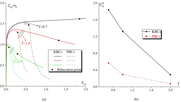
One of the most important issues in terms of ensuring that a homogenization multiscale scheme is accurate and effective is how the boundary conditions are treated. It is well known that KBCs (also called kinematic boundary conditions) require a large representative volume element to accurately capture microscopic properties and phenomena. By contrast, PBCs can provide better evaluations of the microscopic fields and thus of the macroscopic response than uniformly distributed conditions, even for non-periodic geometries (Kanit et al., 2003; Terada et al., 2000; Henyš et al., 2019). Despite its major importance, the effect of boundary conditions on the onset of void coalescence or macroscopic strain localization has not been analyzed in earlier investigations. In fact, a large majority of these investigations use KBCs (Liu et al., 2016) or a mixture of KBCs and PBCs (Barsoum and Faleskog, 2011;Guo and Wong, 2018;Wong and Guo, 2015;Zhu et al., 2018), and a very limited number of contributions is based on fully PBCs. We have conducted a comparative study to investigate the effect of the applied boundary conditions on the distribution of the microscopic fields in an entire sheet made of unit-cell cluster and a single unit cell constrained by PBCs or KBCs. This study confirms the reliability of PBCs compared to KBCs in the prediction of mechanical behavior of the unit cell.
Predictions of the onset of macroscopic strain localization, as given by the bifurcation theory, are then conducted on a 3D unit cell subjected to several proportional stressing states (L 1, T0.7;1.0; 2.0). In this case, the initial volume fractions fp0 (primary void) and
f
s0 (secondary voids) are set to 0.04 and 0.0,respectively. As shown in Fig. 4a, a rapid drop in equivalent stress occurs as the equivalent strain reaches the critical value B
eq
E , indicated by full circles, when the PBCs are used (unlike the curves obtained by the KBCs).
Consequently, strain localization predicted by using KBCs is expected to occur much later than that obtained by PBCs. Fig. 4b shows that E obtained by KBCs is three times higher than that obtained by PBCs. This eqB
figure also demonstrates that KBCs lead to a strong overestimation of the macroscopic equivalent strain at the onset of strain localization.
-20-
(a) (b)
Fig. 4.Effect of the boundary conditions on: (a) the evolution of the equivalent stress eq normalized by the initial yield stress σ0; (b) the evolution of the critical equivalent strain EeqB .
5.3. Proportional stressing
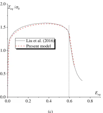
5.3.1. Comparison with results of Liu et al. (2016)
To validate the developed approach, our numerical predictions are compared with those published in Liu et al. (2016). For this purpose, KBCs are applied, instead of PBCs, on the boundary of the unit cell. This unit cell is proportionally stressed, where the stress state is taken to be of T1.0 and L0.0. The onset of void coalescence is predicted by the energy-based criterion presented in Section 4.3. The evolutions of the ratio
/
e p
W W , the macroscopic logarithmic strain components (E11, E22, E33) and the macroscopic equivalent
stress
eq are plotted as functions of the macroscopic equivalent strain Eeq in Fig. 5a, b and c, respectively. Among these plots, our numerical predictions are marked by red curves and those published in Liu et al. (2016)by grey curves. The evolution of the principal logarithmic strains and the equivalent stress–strain response are in very good agreement with those reported in Liu et al. (2016). This is also the case for the predicted value of the critical strain for void coalescence E (eqC EeqC 0.597 in Liu et al., 2016 versus EeqC 0.605 in the current
model). However, the magnitude of e/ p
W W when void coalescence occurs is not in perfect agreement. This
difference is likely to be attributable to the type of the finite element used in the simulations. In fact, the C3D8R element (8-node linear brick element with reduced integration) is used in Liu et al. (2016), while in the present
0.0 0.5 1.0 1.5 2.0 0.0 0.5 1.0 1.5 2.0 KBCs PBCs Bifurcation point T=2.0 T=1.0 eq eq/0 T=0.7 0.8 1.2 1.6 2.0 0.0 0.4 0.8 1.2 1.6 2.0 E B eq T KBCs PBCs
-21-
investigation, the unit cell is discretized by using the C3D8 element. One can observe from the curves of Fig. 5a that, as the unit cell deforms plastically, the energy ratio undergoes a state of decrease up to a point where ratio We/W becomes equal to zero. This means that the loading state applied on the unit cell changes from p
elastoplastic loading to elastic unloading. As further increase in deforming, ratio We/Wp will reach a minimum value where the maximum elastic unloading occurs. This point is identified as the onset of void coalescence. Beyond this point, ratio e/ p
W W will increase from negative to positive. This change means that the mechanical state in the unit cell recovers to elastoplastic loading from elastic unloading. Together with Fig. 5(a), Fig. 5(b) shows a shift of the principal logarithmic strains when void coalescence occurs. It is observed that the cell straining mode shifts from triaxial to uniaxial strain state with E22E330 (Koplik and Needleman, 1988). It is worth noting that the straining mode shifts and the minimum of We/W always p
occurs simultaneously and corresponds to the onset of void coalescence.
(a) (b) 0.0 0.2 0.4 0.6 0.8 -0.03 -0.02 -0.01 0.00 0.01 0.02 0.03 0.04 Eeq Liu et al. (2016) Present model / e p W W 0.0 0.2 0.4 0.6 0.8 -0.6 -0.4 -0.2 0.0 0.2 0.4 0.6 0.8 1.0 E33 E22 E11 Eeq Liu et al. (2016) Present model Eii
-22-
(c)
Fig. 5. Validation of the numerical implementation by comparing our predictions with results published in Liu et al.
(2016): (a) evolution of ratio We/Wp; (b) evolution of the macroscopic logarithmic strain components
11
E , E and 22 33
E ; (c) evolution of the macroscopic equivalent stress eq normalized by the initial stress σ0.
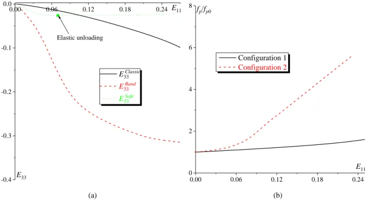
5.3.2. Competition between void coalescence and macroscopic strain localization
To start the analysis of the competition between void coalescence and macroscopic strain localization, three proportional stressing configurations are simulated. For these loadings, the Lode parameter L is set to 1.0 and three values for the stress triaxiality ratio T are considered: 0.8; 1.0 and 2.0. The matrix of the unit cell is assumed to be fully dense (hence, fs00) and the initial volume fraction of the primary void fp0 is set to
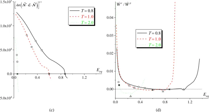
0.04 . The evolution of some macroscopic quantities, relevant to study the competition between void coalescence and macroscopic strain localization, are plotted in Fig. 6. In unit cell computations, the equivalent strain
eq is often used as a measure of material ductility. Therefore, a critical equivalent strain, predicted byeach indicator, has also been used to denote material failure. For comparison purposes, four symbols are marked in each curve of Fig. 6 to designate the level of the macroscopic equivalent strain corresponding to each criterion:
A square ( ) to designate
eqR (when the reaction force component
3 of the dummy node reaches itsmaximum value).
A circle ( ) to designate
eqS (when the equivalent stress
eq reaches its maximum value).0.0 0.2 0.4 0.6 0.8 0.0 0.5 1.0 1.5 2.0 eq /0 Eeq Liu et al. (2016) Present model
-23-
A star ( ) to designate
eqB (when the determinant of the acoustic tensor vanishes).
An up triangle ( ) to designate Ceq (when ratio /
e p
W W reaches its minimum and negative value).
In view of the curves in Fig. 6, some conclusions can be drawn:
For all of the stress triaxiality ratios considered, the critical equivalent strains predicted by the different criteria are classified as follows:.
S R B C
eq eq eq eq
(37)
As expected, the different critical equivalent strains (namely, eqS, eqR, eqB and eqC) decreasewith the increase of stress triaxiality ratio T, reflecting the loss of ductility. Moreover, the dependency of the different critical equivalent strains on T is more pronounced in the low stress triaxiality range and saturates as T increases to a high level.
The difference between the various critical equivalent strains decreases when the stress triaxiality ratio increases. For instance, the difference between eqS and eqC decreases from 0.73 for T0.8 to 0.20 for T2.0.The effect of the stress triaxiality ratio on the onset of ductile failure will be further investigated in Section
5.3.3, where a wide range of T will be considered and not only three particular values.
(a) (b) 0.0 0.4 0.8 1.2 0 1 2 3 4 3 / 0 (mm 2) Eeq 0.0 0.4 0.8 1.2 0.0 0.5 1.0 1.5 2.0 eq / 0 Eeq
-24-
(c) (d)
Fig. 6. Competition between void coalescence and macroscopic strain localization for proportional stressing
configurations defined by T0.8; 1 and 2, with L1: (a) evolution of the reaction force component 3 of the dummy node normalized by the initial stress σ0; (b) evolution of the equivalent stress eq normalized by the initial stress σ0;
(c) evolution of the cubic root of the determinant of the acoustic tensor ; (d) evolution of ratio We/Wp.
5.3.3. Effect of the stress triaxiality ratio on ductile failure
An overview of the competition between void coalescence and strain localization is provided in Fig. 7, where the evolutions of the critical equivalent strains S
eq, R eq, B eq and C
eq are plotted against T for the range
( 0.7 T 3.0) and for three L values (1;
0
and 1.0 ). As one can see, all of the four limit strains decrease as T increases for the different values of L. By examining the evolution of
eqC and
B
eq for a given range
of T , one can observe that eqB eqC regardless the value of L. Namely, localization bifurcation occurs before the attainment of void coalescence predicted by the energy-based criterion for the full range of T. For
2.0
T , the limit strains
eqB,
Req and
Seq are attained with
S R B
eq eq eq, and the difference between
these limit strains decreases as T increases for the various values of L. For higher values of T , notably 2.0
T , the curves corresponding to
eqB,
Req and
Seq are almost indistinguishable. This result means that
for high stress triaxiality levels, the maximum of the reaction force of the dummy node, the maximum equivalent stress and the bifurcation are reached at approximatively the same moment. This latter conclusion
0.0 0.4 0.8 1.2 -5.0x10⁴ 0.0 5.0x10⁴ 1.0x10⁵ 1.5x10⁵ Eeq
1/3 det 0.0 0.4 0.8 1.2 0.00 0.01 0.02 0.03 0.04 Eeq / e p W W-25-
is fully consistent with the predictions obtained by Guo and Wong (2018), where it has been demonstrated that the maximum reaction force of the dummy node (used as strain localization criterion) and the maximum equivalent stress are simultaneously attained for high values of T (typically higher than 1.5). On the other hand, the bifurcation criterion (used in the present contribution as a rigorous macroscopic strain localization criterion) appears to be less conservative than the criterion of maximum reaction force on the dummy node (used as strain localization criterion in Guo and Wong, 2018) for the range of low triaxialty (T2.0), and this is more remarkable for L1.0. Whatever the adopted macroscopic strain localization criterion, defined as the maximum equivalent stress in Bomarito and Warner (2015) and Tekoğlu et al. (2015) or as the maximum reaction force in Guo and Wong (2018), the bifurcation criterion presented herein leads to relatively higher limit strains for T2.0. For higher stress triaxiality ( 2.0 T 3.0), all three strain localization criteria predict almost the same results.
(a) (b) 0.5 1.0 1.5 2.0 2.5 3.0 0.0 0.2 0.4 0.6 0.8 E eq L1 T ECeq EBeq EReq ESeq 0.5 1.0 1.5 2.0 2.5 3.0 0.0 0.2 0.4 0.6 0.8 Eeq T (b) ECeq EBeq EReq ES eq L0
-26-
(c)
Fig. 7. Evolution of critical equivalent strains eqS, eqR, eqB and eqC over the range 0.7 T 3.0 and for (a) L 1; (b) L0; (c) L1.
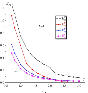
5.3.4. Effect of the Lode parameter on ductile failure
Special attention is now paid to the analysis of the effect of the Lode parameter L on macroscopic strain localization and void coalescence. The evolutions of the critical equivalent strains E and eqC E are plotted in eqB
Fig. 8 over the range 1.0 L 1.0 and for some particular T values (0.8; 1.2; 1.6; 2.0; 2.4 and 3.0). The loci
of C
eq
E and E are denoted by solid and dash lines, respectively. At first glance, it is clear that eqB E is larger eqC
than B
eq
E for the full range of L. For low to moderate levels of T , both C eq
E and B eq
E increase with L,
especially for 0 L 1.0, with different increase rates. Moreover, the difference between C eq
E and B eq E
increases with L in the range 0 L 1.0 for relatively low triaxiality levels. For high stress triaxiality levels (e.g., T2.4 and T3.0), C
eq
E and B eq
E are quasi linear and almost constant for the full range of L. In other
words, the effect of Lode parameter is more pronounced when the stress triaxiality is low. Regarding the effect of L, Barsoum and Faleskog (2011) and Dunand and Mohr (2014) have found that E performs a convex eqC
and non-symmetric function of L ( 1.0 L 1.0) by following the coalescence criterion developed in
Needleman and Tvergaard (1992). This trend has been confirmed by Luo and Gao (2018) using a sandwiched unit cell model, but seems to be inconsistent with that observed in our investigation. This apparent
0.5 1.0 1.5 2.0 2.5 3.0 0.0 0.2 0.4 0.6 0.8 1.0 1.2 Eeq (c) L1 T ECeq EBeq EReq ESeq
-27-
inconsistency is explained by the convention adopted to determine T and L from
1 and
2 (see Section 3.1). In fact, several families of stress states
1, 2
could be obtained from a given T and L, as demonstrated by Wong and Guo (2015). Consequently, for these different stress states, the predicted critical strains for macroscopic strain localization are quite distinct, and the same applies to void coalescence, although the stress triaxiality ratio T and the Lode parameter L remain the same. Therefore, with various stress states
1, 2
, one may draw different conclusions regarding the effect of L (see, e.g., Fig. 11 in Wong and Guo,2015). With the convention for L adopted in our investigation, we obtain trends that are similar to those observed in Zhu et al. (2018).
Fig. 8. Locus of limit strains eqC and B
eq over the range 1.0 L 1.0 and for T0.8; 1.2; 1.6; 2.0; 2.4; 3.0.
-0.8 -0.4 0.0 0.4 0.8 0.0 0.2 0.4 0.6 0.8 1.0 1.2 L Eeq EC eq E B eq T0.8 T1.2 T1.6 T2.0 T2.4 T3.0