Thermoforming of a PMMA transparency near glass transition temperature

Science Arts & Métiers (SAM)

is an open access repository that collects the work of Arts et Métiers Institute of Technology researchers and makes it freely available over the web where possible.

This is an author-deposited version published in: https://sam.ensam.eu Handle ID: .http://hdl.handle.net/10985/6684

To cite this version :

Pierre GILORMINI, Luc CHEVALIER, Gilles REGNIER - Thermoforming of a PMMA transparency near glass transition temperature - Polymer engineering and science p.2004-2012 - 2010

Thermoforming of a PMMA Transparency

near Glass Transition Temperature

Thermoforming of a PMMA Transparency

near Glass Transition Temperature

Authors: P. Gilormini1, L. Chevalier2, G. Régnier1* 1

Laboratoire d’Ingénierie des Matériaux, Arts et Métiers ParisTech, CNRS, 151 boulevard de l’Hôpital, 75013 Paris, France

2

Laboratoire Modélisation Simulation Multi Echelle, Université Paris-Est, CNRS, 5 boulevard Descartes, Champs-sur-Marne, 77 454 Marne-la-Vallée, France *corresponding author, gilles.regnier@paris.ensam.fr

Abstract

In order to simulate the thermoforming of a transparency, constitutive equations are proposed for the nonlinear viscoelastic behaviour of poly(methyl methacrylate) near glass transition temperature, which include large deformations. In a first step, they are fitted on a set of uniaxial tension-relaxation tests at various strain levels and strain rates. In a second step, their implementation in a finite element code is performed. Finally, the thermoforming of a transparency at a constant and uniform temperature is simulated and compared with experimental results.

INTRODUCTION

Transparencies are often made of thermoformed organic sheets to reduce the structure weight. Crosslinked as-cast poly(methyl methacrylate) (PMMA) is generally used for both its good mechanical properties (rigidity, strength to crazing and crack propagation) and its optical properties. To limit optical distortions, PMMA is favourably processed slightly above the glass transition temperature (Tg), at low strain rates. Industry is interested in cheaper and faster tool design, and the technical and economical feasibility of the geometry of transparencies must be validated early in the business phase. Therefore, an accurate model is needed to understand the polymer behaviour during processing and to predict the thickness distribution reliably. This paper presents such a model for the thermoforming of as-cast PMMA transparencies in the above conditions.

Finite element simulations of plastic sheet thermoforming have been performed for more than 20 years to predict the polymer deformation in complex shapes [1]. Several constitutive laws have been used, depending on temperature, polymer state, strain and strain rate. Hyperelastic constitutive equations were initially implemented to predict the deformation above Tg at high strain rates or Deborah numbers. They were generally based on the Mooney-Rivlin equation [2,3] (for plug-assisted thermoforming) or the Ogden model [1,4]. However, the dependence of the stress response on strain rate often could not be neglected. Viscosity has been added to a Mooney-Rivlin constitutive law by Yang et al. [5] to account for the behavior of rubber deformation at high strain rates: the result is in essence similar to a generalized Maxwell model where spring and dashpot have a non linear behavior that depends on strain but not on strain rate. This constitutive law has been applied by Pham et al. [6] to stretch blown molding of PET (polyethylene terephthalate) and by Erchiqui et al. [7] to the thermoforming of PET near glass transition. In these two studies, the hyperelastic behavior also tackles the strain-induced crystallization strain-hardening of PET. Viscoplastic or viscoelastoplastic phenomenological laws, which rather describe the temperature and rate dependences of polymer deformation in the solid state [8,9], have been used to model

thermoforming [10,11]. Even if these models are difficult to justify from a physical point of view, they can describe the stress response of a viscoelastic material in a simple manner with a few adaptive parameters. Moreover, they are easy to compute and lead to stable numerical schemes. K-BKZ (Kaye, Bernstein, Kearsley, Zapas) viscoelastic models have also been used [12, 13], but they fit the polymer deformation behaviour in the flow zone only, and they are not well suited for a thermoforming process near glass transition. Buckley and Jones [14] were among the first to develop a physically based constitutive law in which the stored strain energy is assumed to be the sum of free energies for (a) interatomic (inter- and intramolecular) potentials that refer to “bond distortions”, and (b) perturbation of molecular conformations. This glass-rubber model aims at simulating the processing of amorphous polymers over large ranges of strain rate and temperature, especially near Tg. It has been successfully applied to the creep of PMMA [15] and to the biaxial hot-drawing of PET [16] and PMMA from Tg to 180°C [17], by introducing a spectrum of relaxation times to describe the observed linear viscoelasticity. Revisiting the Argon model [18], Arruda and Boyce [19] keep a nonlinear spring for the deformation of chains network, in parallel with a dashpot to model the yield stress, but they describe the nonlinear spring with their famous eight-chain model for the large stretch of rubber [20]. Numerous researchers have developed variants of this constitutive law, among which Karamanou et al. [21] and Richeton et al. [22]. However, these constitutive laws are more suited to model the behaviour of amorphous polymers below and near the glass transition. For stress relaxation at higher temperatures, Hernandez et al. [23] pointed out that there does not exist a single relaxation time, but rather two distributions of relaxation times. Quite recently, Dupaix and Boyce [24] developed a three-dimensional constitutive law that is based on two mechanisms: (a) the intermolecular interactions between neighbouring chain segments, which are the primary source of the initial stiffness and saturate at a finite stress in plastic flow, and (b) the deformation of the molecular network and the orientation of the chains, which also contribute to the initial stiffness but, more importantly, induce a stiffening at large strains. This constitutive law was used to model the thermoforming of PMMA by Makradi et al.

[25]. This is also the type of approach that is adapted to crosslinked PMMA in the present paper. However, it cannot model easily the back stress that is observed experimentally after the yield point in the glassy state or close to Tg. Hasan and Boyce [26] explained this phenomenon by local heterogeneities at nano scale, but this is still not very clear. Anand et al. [27] modified the model to account in a phenomenological manner for Bauschinger-like effects, by replacing the viscous part of intermolecular interactions by a viscoelastic part, and Ames et al. [28] used this model to simulate the hot embossing and the thermoforming of PMMA, polycarbonate, and polycycloolefins. This paper describes the simulation of the thermoforming of a crosslinked as-cast PMMA transparency at a constant temperature close to Tg, at moderate strain and strain rate. The paper is organized as follows. First, tension-relaxation tests on PMMA are presented, and the identification of the three-dimensional constitutive law is deduced. Then, the numerical implementation is described, and the simulation of the thermoforming of a transparency is discussed and compared with experiments.

MODELING THE PMMA BEHAVIOUR NEAR GLASS TRANSITION TEMPERATURE Tension-relaxation tests on PMMA near glass transition temperature

In order to perform tension-relaxation tests, specimens were cut off from as-cast PMMA sheets of 5 mm thickness. The glass transition temperature measured by differential scanning calorimetry at 10 K/min is 118°C and the tests were performed at 120 and 125°C, since the material is processed within this temperature range. The tensile tests were performed with a specific strain history in order to stay as close as possible to the process conditions.

The specimens were 25 mm wide and 150 mm long, with a useful initial length of 100 mm, and tensile tests were carried out on a hydraulic testing machine MTS Elastomer Test System 831. Thermal regulation was managed by convection in an oven that covered the specimen and the grips. Because the PMMA used was not completely relaxed, the specimens were placed in an oven at 150°C before testing. To stay close to the process conditions, the tension-relaxation tests were

divided into 3 steps: first (heating step), the load was regulated to zero and temperature was increased from ambient to test temperature; then (tension step), temperature was kept constant and the specimen was stretched from 0 to a prescribed

ε

0 strain at a constant strain rate; finally

(relaxation step), the strain was kept constant and a decreasing tensile force was recorded. In what follows,

ε

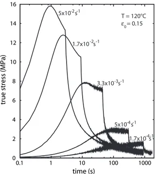
0 is equal to 0.15, and therefore the cross section of the specimen is corrected to obtain the true stress values shown in Fig. 1. In this figure, where five strain rate values are applied at 120°C, the behaviour is clearly nonlinear: the strain rate is multiplied by 3 between the lowest and the second curve, whereas the maximum stress doubles approximately; the same strain rate ratio is applied between the two upper curves, and the stress is multiplied by 1.2.

The tests have been repeated at least three times to ensure the repeatability of the behaviour, and less than 0.5 MPa stress dispersion was observed. Since the plots for the tension steps superimpose very well, a single typical curve is chosen and presented in Fig. 1 for each strain rate. Three

ε

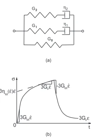
0 values have been applied: 0.05, 0.10, and 0.15. A log scale is used along the time axis and it can be observed that the relaxation response differs from the decreasing straight line that would be given by a simple Maxwell model. This could be expected by noting that several physical mechanisms are involved simultaneously, each with a different characteristic time. One can also observe that the stress decreases quickly but does not tend to zero: the persistent stress is due to the elasticity of the rubber-like network (recall that strain is maintained to a nonzero value). The rheological model needs at least three branches (see Fig. 2a) to represent the experimental behaviour of PMMA at 120°C accurately: G0 defines the elastic shear modulus of the rubber-like network, and the two other branches account for the viscoelastic behaviour that involves two relaxation times, as suggested by Dupaix and Boyce [24]. Assuming the material is incompressible leads to the factors of 3 that appear in the tensile test sketched in Fig. 2b.

As illustrated in Fig. 2b, G0 can be obtained from the asymptotic stress value at the end of the relaxation step (the slope at the end of the tension step could alternatively be used), the sum of the two other elastic parameters has been deduced from both the slope (Gtot=G0+G1+G2) at the

beginning of the tension step and the slope at the beginning of the relaxation step. The values of G0 and Gtot deduced from the tension-relaxation tests did not vary significantly with temperature and strain rate. The mean values of Gtot and G0 have been chosen over the set of tests done at 120 and 125°C; the standard deviations were 23 MPa and 0.2 MPa, respectively. This confirms the consistency of the model and allows using constant elastic properties in the simulations below, which involve temperatures and strain rates in the same ranges.

The sum of the two viscous parameters (

η

tot=

η

1+

η

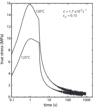
2) has been obtained by back extrapolating the end of the tension step. In contrast, the viscous parameters were found to depend strongly on both strain rate and temperature, and the latter trend is illustrated in Fig. 3. The effect of temperature could be accounted for satisfactorily via a William-Landel-Ferry (WLF) model, and the influence of strain rate via a Carreau model, as shown in Fig 4. Simply taking

η

1=

η

2 lead to a partitioning of

η

tot that provided a good and easy fit of the model, as shown below. Finally, the balance between G1 and G2, which defines the two relaxation times, has been tuned by fitting the curvature from the initial elastic part to the final asymptotic part of the relaxation step.

Constitutive equations for PMMA near glass transition temperature

A three-dimensional nonlinear viscoelastic behaviour has been written that is suitable for PMMA near glass transition and at large deformations. The model generalizes the usual assembly of parallel linear Maxwell branches that is used at infinitesimal strains, with two modifications: (i) the constant viscosity of the viscous components now depends on the viscous strain rate;

(ii) small strain elasticity is replaced by a hypoelastic law that relates the stress increment to the elastic strain increment.

The latter point leads to substantial simplifications when large deformations, including large rotations especially, are considered, with negligible differences obtained with respect to significantly more complex hyperelastic laws (where an elastic strain energy function is defined) when elastic strains keep small, as is the case in the applications considered here.

Therefore, the constitutive equations that are used write as follows, since two viscous branches are enough to describe the polymer considered:

) , ( 2 2 ) , ( 2 2 2 (2) ) 2 ( 2 ) 2 ( ) 1 ( ) 1 ( 1 ) 1 ( 0 ) 0 ( T e G T e G G

η

&

η

& s s s s s D_{= = + = +} ∇ ∇ ∇ (1)

where D denotes the Eulerian strain-rate (i.e. the symmetric part of the gradient of the velocity field), which is trace free in the present case (assuming the PMMA is incompressible), s(0) _{is the}

deviatoric stress in the elastic branch, s(1) _and s(2) _{are the deviatoric stresses in the two viscous}

branches (the total deviatoric stress being given by s₌s(0) ₊s(1) ₊s(2)_{). In the present large}

deformation context, Green-Naghdi derivatives ∇ ) 0 ( s _, ∇ ) 1 ( s _and ∇ ) 2 (

s _{are used, with the standard}

definition s(k) ₌s(k) ₊s(k)_Ω−Ωs(k)

∇

& with _Ω=R& R−1_{, where R is the rotation obtained from the}

polar decomposition of the transformation gradient F₌RU_{, and a dot denotes the usual time}

derivative. The equivalent viscous strain rate is defined as e_{& =}(k) 2e_&(k):e_&(k)/3_{, where} e_{& is the} (k)

deviatoric viscous strain rate in a branch. The elastic shear moduli of the branches are G₀, G₁, and

2

G , while η is the viscosity defined in terms of viscous strain rate e& and temperature T as the same combination of Carreau and Williams-Landel-Ferry models in both branches (with η=η1=η2):

a m a WLF WLF e T T T e 1 ) ( 1 2 ) ( ) , ( −               + = & & ξ η η η with _{0 1} 2 ( ) exp r WLF r T T T C C T T

η

=

η

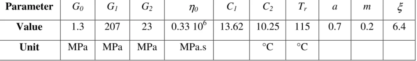
− −  + −   (2)

where the factor 2 is the number of viscous branches considered. The complete set of constitutive equations involves 10 materials constants:G₀, G₁, G₂, η₀, C₁, C₂, Tr, a, m, and ξ. These

constants were fitted on the series of uniaxial tension-relaxation tests described above, using a Matlab integration of the set of constitutive equations, which was easy since the strain history was prescribed in the tests. Following the guidelines given in the preceding section, an identification of the model parameters G0, G1, G2 and η0 has been performed, which lead to the numerical values

given in Table 1. It may be noted that, due to the values of G1 and G2, two relaxation times are obtained with a ratio of about 10, which is consistent with previous results [23] and with very different physical mechanisms being involved.

SIMULATION OF THE THERMOFORMING OF A TRANSPARENCY Numerical implementation

The above constitutive equations have been implemented in the Abaqus (from Dassault Systems Simulia) finite element code as a Fortran user material (UMAT) routine. This routine updates the total stress and computes the consistent tangent modulus for any strain increment defined by three components only, since shell elements are used in the simulations: ∆

ε

₁₁, ∆

ε

₂₂, and ∆

ε

₁₂, with axis 3 being normal to the shell. It can be checked readily that using shell elements with a UMAT routine implies that the orthogonal axes 1 and 2 used to define tensor component rotate with R . This leads to significant simplifications, since taking a Green-Naghdi derivative amounts to taking usual time derivatives of all components in the rotating frame defined locally by axes 1 and 2. Similarly, running such examples as simple shear with a single element shows immediately that the strain used by the UMAT routine is merely the integral of the strain rate in this rotating frame and, therefore, one has ∆εij = Dij∆t where the components (on the rotating local

axes 1 and 2) of the average strain rate during the time increment are denoted by D_ij. This is the key to the analysis that follows.

With the above considerations, one has immediately

ij ij ij ij ij t t s t s s t G s(0) +∆ = (0) +∆ (0) = (0) + ₀∆

ε

2 ) ( ) ( ) ( ij=11, 22, 12 (3)

for the elastic branch, since the strain increment is purely elastic in this branch, but applying (1) to a viscous branch is less trivial because the strain increment splits into elastic and viscous parts with a priori unknown weights. Consider branch 1, for instance. Since the main unknown is the increment

of deviatoric stress in the branch, the viscosity is rewritten in terms of stress rather than viscous strain rate. This can be obtained by using the basic relation s(1) ₌2_η(_e&(1),_T)e_&(1) _{that leads to}

) 1 ( ) 1 ( ) 1 ( ) , ( 3 e T e

s = η & & , where _s(1) ₌ 3s(1) :s(1)/2 _{denotes the equivalent stress in the branch, and} combining with (2) this allows defining η(s(1),T) for any positive value of s(1) through a numerical procedure (a simple fixed-point method proves very efficient in the present case). Therefore, (1) can be rewritten as ) , ( 2 ) 1 ( ) 1 ( 1 1 T s G G η s D s_{= −} ∇ (4)

for branch 1, which can be discretized with a centered-difference scheme to obtain eventually

(

)

(

)

      _∆ − ∆ ∆ + = ∆ (1) ) 1 ( ) 1 ( 1 1 ) 1 ( , ~ 2 , ~ 2 1 2 ij ij ij s T s t T s t G G s

η

ε

η

ij=11, 22, 12 (5)

where ~s(1) denotes the equivalent stress in the branch at t+∆t and, consequently, depends on the unknown ∆s_ij(1). The nonlinear system (5) of three equations with respect to the three unknowns

) 1 ( 11

s

∆ , ∆s₂₂(1), and ∆s₁₂(1) can be combined into a single nonlinear equation with respect to the unknown ~s(1). It is easily solved with a fixed-point method, and this finally leads to the updated deviatoric stress in branch 1. A similar system is solved for branch 2, and finally the updated deviatoric stress at the integration point is obtained as

) 2 ( ) 1 ( ) 0 ( ) ( ) ( _{ij ij ij ij} ij t t s t s s s s +∆ = +∆ +∆ +∆ ij=11, 22, 12. (6)

The above procedure implies that the deviatoric stress in each viscous branch is stored, in order to be available at the beginning of the next increment, and this is performed by defining 6 internal variables (3 components per branch) in the UMAT routine, at each integration point. It may also be noted that computing the equivalent stress implies knowing all the 5 independent components of the deviatoric stress in each branch, and the free surface conditions σ₁₃ =σ₂₃ =0

are used in branch k to prescribe ₁₃(k) = ₂₃(k) =0

s

s . The last free surface condition σ₃₃ =0 gives the hydrostatic pressure p=−s11 −s22, which leads to the following expressions for the updated nonzero total stress components:

σ

11 =2s11 +s22,

σ

22 =s11+2s22, and

σ

12 =s12.

Finally, the consistent tangent modulus must be computed in the UMAT routine, in order to allow an efficient iterative procedure over the whole mesh, and this has been performed very simply by running the core of the routine three times, with a single component of the strain increment slightly modified in each case. This numerical evaluation of the Jacobian matrix proved very efficient, since convergence was obtained rapidly in the applications described in the next section.

It may be noted that the model, as well as its numerical implementation, is modular and can include as many viscous branches as wished. Moreover, the approach is quite flexible, since modifying the nonlinear behaviour in the viscous branches amounts merely to adapting the subroutine where η(s(k),T) is computed by a fixed-point method. Prior to the simulations described below, the UMAT routine has been tested in two ways, successfully: on a single element by simulating the uniaxial relaxation tests used above to identify the material behaviour, and on more complex structures, by choosing the material parameters so as to get a linear viscoelastic behaviour in order to compare with using the standard viscoelastic routine of the finite element code.

Simulation of thermoforming and discussion

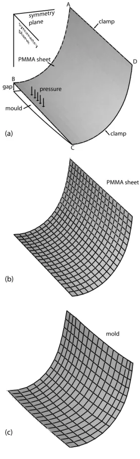
Before thermoforming is performed, the as-received flat PMMA sheet, which is 8.5 mm thick, is rolled to get the shape of an elliptical cylinder. Since the latter is a developable surface, this preliminary forming process does not induce any significant thickness change and is assumed to have no influence on the properties of the material, consequently. The rolled PMMA piece used to form the transparency is 1.6 m long, 0.8 m wide, and 0.6 m high. The mold and the rolled PMMA piece were slowly heated in an oven; temperature was measured and remained constant during the process. Therefore, the problems usually induced by a fast heating of the part with the subsequent need to know an initial nonuniform temperature field [29] are not relevant here. For symmetry

reasons, one quarter of the transparency and the die is considered in the simulations, as shown in Fig. 5. The mesh uses 361 quadrilateral shell elements with reduced integration for the sheet, with a uniform initial thickness of 8.5 mm, and 208 quadrilateral rigid elements for the die surface. Since the die was lubricated, frictionless contact conditions are applied in the simulations. The Abaqus/Standard finite element code is used, which solves an implicit set of equations iteratively in order to ensure mechanical equilibrium at the end of each time increment. This iterative procedure uses a global stiffness matrix that is formed in part from the consistent tangent modulus defined in the UMAT routine. The code has elaborate internal procedures to optimize the time increment and to tackle large deformation, shell element formulation, and part-mold contact, so that the user can concentrate on constitutive equations.

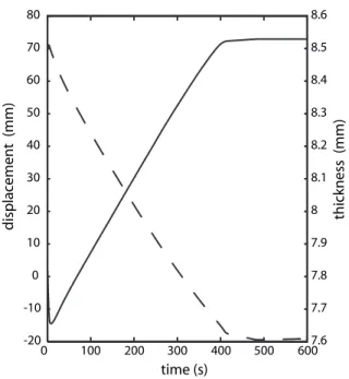
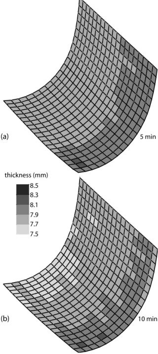
As shown in Fig. 5a, the sheet edges are clamped to the die and everywhere else there is a gap through which the applied pressure will move the sheet towards the die during the thermoforming process. The pressure is increased linearly from zero during the first 5 seconds of the process, and then it is maintained constant at its nominal value of 0.5 bar. Fig. 6 illustrates the history of a typical point, namely point B shown in Fig. 5. It may be noted that point B moves downwards (negative displacement), i.e. the gap between the sheet and the die increases, during the first 10 seconds of the process. This is due to the clamping of the sheet, which induces a rotation of the sheet elements near the edges. In a second stage, point B follows the same trend as all points, with an almost linearly decreasing gap between sheet and die, coming along with a less linearly decreasing thickness. In this simulation, point B contacts the die after 490 s, and this also corresponds to the stabilization of thickness. The thickness variations over the whole sheet are illustrated in Fig. 7 after 5 minutes and 10 minutes forming times, where lighter shades of grey correspond to smaller thicknesses. Of course, smaller thicknesses are obtained when the forming process is closer to its end, and thickness heterogeneities can be observed, with a thinner area covering the central part of the transparency.

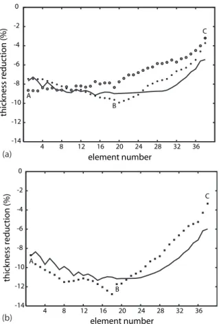
The thickness of the transparency is an important quality parameter, and it has been measured along the two symmetry lines AB and BC shown in Fig. 5a, on several transparencies where the thermoforming process either was interrupted after 10 minutes of applied pressure, or was complete. The measures were performed at places that corresponded to the AB and CD rows of 19 elements used in the simulations, in order to make comparisons easier. As can be observed in Fig. 8a, for incomplete forming, the measured values differ somewhat when two series of results, obtained on different transparencies, are compared. This discrepancy compares well with the differences between experiments and simulations, as can be observed in Figs 8a and 8b. Of course, the natural trend of lower thicknesses for longer forming times is obtained when comparing Figs 8a and 8b. Therefore, the general agreement obtained allows concluding that the predictions are quite satisfactory as far as the transparency thickness is concerned.

Residual stresses have not been mentioned by our industry partners as a key problem for this type of thermoforming, probably because of the low rubbery modulus and of the slow cooling in the oven that allows stress relaxation. Therefore, the shape stability of the transparencies is ensured as long as the in-use temperature remains significantly below Tg.

CONCLUDING REMARKS

The thermoforming simulation of an as-cast PMMA transparency slightly above glass transition temperature was conducted using the finite element method. The mechanical behaviour of the material was described by a nonlinear viscoelastic constitutive law by generalizing the usual assembly of parallel “spring-dashpot” branches with a viscosity that depends on strain rate and temperature. The procedure used to identify the parameters showed that two viscoelastic branches and one elastic branch, to account for the rubbery behavior of the crosslinked polymer, are sufficient to get a good fit of the uniaxial tension-relaxation tests except for the back stress after the yield point, which would need additional developments. The general agreement between measured and predicted thicknesses allows beginning to use this thermoforming simulation as a predictive

tool for industrial applications. Since the polymer sheet may slip on the die surface, which is likely to affect the local deformation and thickness, the very simple frictionless contact law used here should be improved if necessary. The whole methodology can be extended to the simulation of most amorphous polymer forming processes near glass transition and at low strains rates.

NOMENCLATURE

a first exponent of the Carreau model

C1 , C2 coefficients of WLF model

D , Dij Eulerian strain-rate tensor and its components

) (k

e

& , (k)

e& deviatoric viscous strain rate tensor and equivalent viscous strain rate in branch k

F _{deformation gradient tensor}

Gk , Gtot shear modulus of branch k, total shear modulus

m second exponent of the Carreau model

p hydrostatic pressure

R _{rigid body rotation tensor}

) ( ~k

s equivalent stress in branch k at t+∆t

s , sij total deviatoric stress tensor and its components

) (k

s , s(k) deviatoric stress tensor and equivalent stress in branch k )

(k

ij

s , ∆s(kij) components of the deviatoric stress tensor in branch k and their increments

∇ ) ( k

s _, s_& ( k) _{Green-Naghdi derivative and material time derivative of tensor} s( k) t , ∆t time and time increment

T , Tg , Tr temperature, glass transition temperature, reference temperature

U _{right stretch tensor}

∆εij , ε0 components of the increment of total strain, prescribed uniaxial strain

η , ηk , ηtot viscosity, viscosity in branch k, total viscosity

ηWLF, η0 viscosity and reference viscosity in the WLF model

σij components of the total stress

ξ parameter of the WLF mode Ω

Ω Ω

Ω spin tensor

Acknowledgements

The authors acknowledge E. Barselotti and T. Chalutaud for their contributions in the identification procedure and the simulations.

REFERENCES

1. K. Kouba, O. Bartos, and J. Vlachopoulos, Polym. Engng Sci., 32, 699 (1992). 2. P. Bourgin, I. Cormeau, and T. Saint-Matin, J. Mater. Process. Technol., 54,1 (1995). 3. G.N. Nam, J.W. Lee, and K.H. Ahn, Polym. Engng Sci., 40, 2232 (2000).

4. Y. Dong, R.J.T. Lin, and D. Bhattacharyya, J. Mater. Sci., 40, 399 (2005). 5. L.M. Yang, V.P.W. Shim, and C.T. Lim, Int. J. Impact Engng, 24, 545 (2000). 6. X.T. Pham, F. Thibault, and L.T. Lim, Polym. Engng Sci., 44, 1460 (2004). 7. F. Erchiqui, M. Souli, and R. Ben Yedder, Polym. Engng Sci., 47, 2129 (2009). 8. C. G'sell and J.J. Jonas, J. Mater. Sci., 14, 583 (1979).

9. C. G'Sell and A. Souahi, J. Engng Mater. Technol., 119, 223 (1997).

10. M. Bellet, M.H. Vantal, and B. Monasse, Int. Polym. Process., 13, 299 (1998). 11. G. Sala, L. Di Landro, and D. Cassago, Mater. Design, 23, 21 (2002).

12. P. Novotný, P. Sáha, and K. Kouba, Int. Polym. Process., 14, 291 (1999)

13. P. Collins, J.F. Lappin, E.M.A. Harkin-Jones, and P.J. Martin, Plastics Rubber Composites

Process. Appl., 29, 349 (2000).

14. C.P. Buckley and D.C. Jones, Polymer, 36, 3301-3312 (1995).

15. P.J. Dooling, C.P. Buckley, and S. Hinduja, Polym. Engng Sci., 38, 892 (1998). 16. A.M. Adams, C.P. Buckley, and D.P. Jones, Polymer, 39, 5761 (1998).

17. P.J. Dooling, C.P. Buckley, S. Rostami, and N. Zahlan, Polymer, 43, 2451 (2002). 18. A.S. Argon, Phil. Mag., 28, 839 (1973).

19. E.M. Arruda and M.C. Boyce, Int. J. Plasticity, 9,783 (1993).

20. E.M. Arruda and M.C. Boyce, J. Mech. Phys. Solids, 41, 389 (1993).

21. M. Karamanou, M.K. Warby, and J.R. Whiteman, Comput. Meth. Appl. Mech. Engng, 195, 5220 (2006).

22. J. Richeton, S. Ahzi, K.S. Vecchio, F.C. Jiang, and A. Makradi, Int. J. Solids Struct., 44, 7938 (2007).

23. A. Hernandez-Jimenez, J. Hernandez-Santiago, A. Macias-Garcia, and J. Sanchez-Gonzalez,

Polymer Testing, 21, 325 (2002).

24. R.B. Dupaix and M.C. Boyce, Mech. Mater., 39, 39 (2007).

25. A. Makradi, S. Belouettar, S. Ahzi, and S. Puissant, J. Appl. Polym. Sci., 106, 1718 (2007). 26. O.A. Hasan and M.C. Boyce, Polym. Engng Sci., 35, 331 (1995).

27. L. Anand, N.M. Ames, V. Srivastava, and S.A. Chester, Int. J. Plasticity, 25, 1474 (2009). 28. N.M. Ames, V. Srivastava, S.A. Chester, and L. Anand, Int. J. Plasticity, 25, 1495 (2009). 29. F. Erchiqui, I. Hamani, and A. Charette, Int. J. Thermal Sci., 48, 73 (2007).

Figure Captions

Figure 1: Stress history measured during tension-relaxation tests at different strain rates, for ε0=0.15 at 120°C.

Figure 2: Rheological model for the viscoelastic behaviour of PMMA near glass transition. Three branches are needed for an accurate account of the nonlinear strain rate effects. Here, ηtot=η1+η2 and Gtot=G0+G1+G2.

Figure 3: Stress history measured during tension-relaxation tests at different temperatures and at the same strain rate.

Figure 4: Experimental values of the viscosity (ηtot=η1+η2) obtained from tension-relaxation tests at 120°C and 125°C (symbols), which are fitted to a Carreau model (curves) coupled to a WLF model for temperature effects.

Figure 5: Initial configuration of the sheet and die (a), only one quarter is shown and symmetry planes are indicated. Meshes used in the finite element simulations for the sheet (b) and die (c).

Figure 6: History of the vertical displacement (unbroken line) and sheet thickness (broken line) at point B.

Figure 7: Sheet thickness computed after 5 min (a) and 10 min (b) forming times.

Figure 8: Thickness variations measured (symbols) and calculated (lines) along the AB and BC symmetry lines, after (a) 10 min thermoforming (two transparencies) and (b) complete

Parameter _{G0 G1 G2 η0 C1 C2 Tr a m ξ} Value _{1.3 207 23 0.33 10}6 _{13.62 10.25 115 0.7 0.2 6.4}

Unit _{MPa MPa MPa MPa.s °C °C}

0 2 4 6 8 10 12 14 16 0.1 1 10 100 1000

true stress (MPa

) time (s) T = 120°C ε = 0.15₀ 5x10 s-4 -1 1.7x10 s-4-1 3.3x10 s-3 -1 5x10 s-2 -1 1.7x10 s-2 -1

Figure 1: Stress history measured during tension-relaxation tests at different strain rates, for ε0=0.15 at 120°C.

G1 G0 G2 η2 η₁ t σ 3η (ε)ε 3_{G ε} . . . 0 o (a) (b) tot -3G εtot. 3G εtot. 3G εo

Figure 2: Rheological model for the viscoelastic behaviour of PMMA near glass transition. Three branches are needed for an accurate account of

0 2 4 6 8 10 12 14 16 0.1 1 10 100 1000

true stress (MPa

) time (s) 120°C 125°C ε = 0.15₀ ε = 1.7 x10 s. -2 -1

Figure 3: Stress history measured during tension-relaxation tests at different temperatures and at the same strain rate.

10 1 10-1 10 104 103 105 10-2 10-3 10-4 10-5 10-6 strain rate (s ) visc o sit y (M Pa .s) 120°C 125°C 2 -1

Figure 4: Experimental values of the viscosity (ηtot=η1+η2) obtained from tension-relaxation tests at 120°C and 125°C (symbols), which are fitted to a Carreau model (curves) coupled to a WLF model for temperature effects.

clamp clamp mould PMMA sheet gap _pressure sym met ry pla ne symmetry plane A B C D (a) (b) (c) PMMA sheet mold

Figure 5: Initial configuration of the sheet and die (a), only one quarter is shown and symmetry planes are indicated. Meshes used in

-20 -10 0 10 20 30 40 50 60 70 80 0 100 200 300 400 500 6007.6 7.7 7.8 7.9 8 8.1 8.2 8.3 8.4 8.5 8.6 displacement (m m) thic knes s (mm ) time (s)

Figure 6: History of the vertical displacement (unbroken line) and sheet thickness (broken line) at point B.

5 min 10 min 7.5 7.7 7.9 8.1 8.3 8.5 thickness (mm) (a) (b)

-14 -12 -10 -8 -6 -4 -2 0 4 8 12 16 20 24 28 32 36 thickness reducti on ( %) element number (a) A B C -14 -12 -10 -8 -6 -4 -2 0 4 8 12 16 20 24 28 32 36 thickness reducti on (%) element number (b) A B C

Figure 8: Thickness variations measured (symbols) and calculated (lines) along the AB and BC symmetry lines, after (a) 10 min thermoforming (two transparencies) and