Inferring Streaming Video Quality from Encrypted Traffic: Practical Models and Deployment Experience

HAL Id: hal-02268404

https://hal.inria.fr/hal-02268404

Preprint submitted on 20 Aug 2019

HAL is a multi-disciplinary open access

archive for the deposit and dissemination of

sci-entific research documents, whether they are

pub-lished or not. The documents may come from

teaching and research institutions in France or

abroad, or from public or private research centers.

L’archive ouverte pluridisciplinaire HAL, est

destinée au dépôt et à la diffusion de documents

scientifiques de niveau recherche, publiés ou non,

émanant des établissements d’enseignement et de

recherche français ou étrangers, des laboratoires

publics ou privés.

Inferring Streaming Video Quality from Encrypted

Traffic: Practical Models and Deployment Experience

Paul Schmitt, Francesco Bronzino, Sara Ayoubi, Guilherme Martins, Renata

Teixeira, Nick Feamster

To cite this version:

Paul Schmitt, Francesco Bronzino, Sara Ayoubi, Guilherme Martins, Renata Teixeira, et al.. Inferring

Streaming Video Quality from Encrypted Traffic: Practical Models and Deployment Experience. 2019.

�hal-02268404�

Inferring Streaming Video Quality from Encrypted Traffic:

Practical Models and Deployment Experience

Paul Schmitt

, Francesco Bronzino

, Sara Ayoubi

,

Guilherme Martins

, Renata Teixeira

, and Nick Feamster

◦

Princeton University ∗Inria, Paris

Abstract

Inferring the quality of streaming video applications is important for Internet service providers, but the fact that most video streams are encrypted makes it difficult to do so. We develop models that in-fer quality metrics (i.e., startup delay and resolution) for encrypted streaming video services. Our paper builds on previous work, but extends it in several ways. First, the model works in deployment settings where the video sessions and segments must be identi-fied from a mix of traffic and the time precision of the collected traffic statistics is more coarse (e.g., due to aggregation). Second, we develop a single composite model that works for a range of different services (i.e., Netflix, YouTube, Amazon, and Twitch), as opposed to just a single service. Third, unlike many previous mod-els, the model performs predictions at finer granularity (e.g., the precise startup delay instead of just detecting short versus long de-lays) allowing to draw better conclusions on the ongoing streaming quality. Fourth, we demonstrate the model is practical through a 16-month deployment in 66 homes and provide new insights about the relationships between Internet “speed” and the quality of the corresponding video streams, for a variety of services; we find that higher speeds provide only minimal improvements to startup delay and resolution.

1

Introduction

Video streaming traffic is by far the dominant application traffic on today’s Internet, with some projections forecasting that video streaming will comprise 82% of all Internet traffic in just three years [13]. Optimizing video delivery depends on the ability to determine the quality of the video stream that a user receives. In contrast to video content providers, who have direct access to video quality from client software, Internet Service Providers (ISPs) must infer video quality from traffic as it passes through the network. Unfortunately, because end-to-end encryption is becoming more common, as a result of increased video streaming content over HTTPS and QUIC [28, 30], ISPs cannot directly observe video qual-ity metrics such as startup delay, and video resolution from the video streaming protocol [5, 17]. The end-to-end encryption of the video streams thus presents ISPs with the challenge of inferring video quality metrics solely from properties of the network traffic that are directly observable.

Previous approaches infer the quality of a specific video service, typically using offline modeling and prediction that is based on an offline trace in a controlled laboratory setting [14, 22, 26]. Unfor-tunately, these models are often not directly applicable in practice because practical deployments (1) have other traffic besides the video streams themselves, creating the need to identify video ser-vices and sessions; (2) have multiple video serser-vices, as opposed

to just a single video service. Transferring the existing models to practice turns out to introduce new challenges due to these factors. First, inference models must take into account the fact that real network traffic traces have a mix of traffic, often gathered at coarse temporal granularities due to monitoring constraints in production networks and video session traffic is intermixed with non-video cross-traffic. In a real deployment, the models must identify the video sessions accurately, especially given that errors in identifying applications can propagate to the quality of the prediction models. Second, the prediction models should apply to a range of services, which existing models tend not to do. A model that can predict qual-ity across multiple services is hard because both video streaming algorithms and content characteristics can vary significantly across video services (e.g., buffer-based [20] versus throughput-based [33] rate adaption algorithm, fixed-size [20] versus variable-size video segments [27]).

This work takes a step towards making video inference models practical, tackling the challenges that arise when the models must operate on real network traffic traces and across a broad range of services. As a proof of concept that a general model that applies across a range of services in a real deployment can be designed and implemented, we studied four major streaming services—Netflix, YouTube, Amazon, and Twitch—across a 16-month period, in 66 home networks in the United States and France, comprising a total of 216,173 video sessions. To our knowledge, this deployment study is the largest public study of its kind for video quality inference.

We find that models that are trained across all four services (com-posite models) perform almost as well as the service-specific models that were designed in previous work, provided that the training data contains traffic from each of the services for which quality is being predicted. On the other hand, we fall short of developing a truly general model that can predict video quality for services that are not in the training set. An important challenge for future work will be to devise such a model. Towards the goal of developing such a model, we will release our training data to the community, which contains over 13,000 video sessions labeled with ground truth video quality, as a benchmark for video quality inference, so that others can compare against our work and build on it.

Beyond the practical models themselves, the deployment study that we performed as part of this work has important broader im-plications for both ISPs and consumers at large. For example, our deployment study reveals that the speeds that consumers purchase from their ISPs have considerably diminishing returns with respect to video quality. Specifically, Internet speeds higher than about 100 Mbps of downstream throughput offer only negligible improve-ments to video quality metrics such as startup delay and resolution. This new result raises important questions for operators and con-sumers. Operators may focus on other aspects of their networks to

optimize video delivery; at the same time, consumers can be more informed about what downstream throughput they actually need from their ISPs to achieve acceptable application quality.

The rest of the paper proceeds as follows. Section 2 provides background on streaming video quality inference and details the state of the art in this area; in this section, we also demonstrate that previous models do not generalize across a range of services. Section 3 details the video quality metrics we aim to predict, and the different classes of features that we use as input to the predic-tion models. Secpredic-tion 4 explains how we selected the appropriate prediction model for each video quality metric and how we trained the models. Section 5 discusses the model validation and Section 6 describes the results from the 16-month, 66-home deployment. Sec-tion 7 concludes with a summary and discussion of open problems and possible future directions.

2

Background and Related Work:

Streaming Video Quality Inference

In this section, we first provide background on DASH video stream-ing. Then, we discuss the problem of streaming video quality infer-ence that ISPs face, and the current state of the art in video quality inference.

Internet video streaming services typically use Dynamic Adap-tive Streaming over HTTP (DASH) [32] to deliver a video stream. DASH divides each video into time intervals known assegments or chunks (of possibly equal duration), which are then encoded at multiple bitrates and resolutions. These segments are typically stored on multiple servers (e.g., a content delivery network) to allow a video client to download segments from a nearby server. At the beginning of a video session, a client downloads a DASH Media Presentation Description (MPD) file from the server. The MPD file contains all of the information the client needs to retrieve the video (i.e., the audio and video segment file information). The client se-quentially issues HTTP requests to retrieve segments at a particular bitrate. Anapplication-layer Adaptive Bitrate (ABR) algorithm deter-mines the quality of the next segment that the client should request. ABR algorithms are proprietary, but most video services rely on recently experienced bandwidth [33], current buffer size [20], or a hybrid of the two [37] to guide the selection. The downloaded video segments are stored in a client-side application buffer. The video buffer is meant to ensure continuous playback during a video session. Once the size of the buffer exceeds a predefined threshold, the video starts playing.

ISPs must infer video quality based on the observation of the packets traversing the network. The following video quality metrics affect a user’s quality of experience [2, 6, 7, 15, 16, 21, 23]:

• Startup delay is the time elapsed from the moment the player initiates a connection to a video server to the time it starts rendering video frames.

• The resolution of a video is the number of pixels in each dimension of video frame.

• The bitrate of a segment measures the number of bits trans-mitted over time.

• Resolution switching has a negative effect on quality of expe-rience [6, 19]; both the amplitude and frequency of switches affect quality of experience [19].

Netflix

YouTube

Amazon

0

20

40

60

80

Percentage

FP Rate

Precision

Recall

Figure 1: Using a per-service model to detect high (bigger than 5 seconds) startup delay using method from Mazhar and Shafiq [26].

• Rebuffering also increases rate of abandonment and reduces the likelihood that a user will return to the service [15, 23]. Resolution and bitrate can vary over the course of the video stream. Players may switch the bitrate to adapt to changes in network conditions with the goal to select the best possible bitrate for any given condition.

In the past, ISPs have relied on deep-packet inspection to identify video sessions within network traffic and subsequently infer video quality [24, 31, 36]. Yet, most video traffic is now encrypted, which makes it more challenging to infer video traffic [5, 17].

Previous work has attempted to infer video quality from en-crypted traffic streams, yet has typically done so (1) in controlled settings, where the video traffic is the only traffic in the experiment; (2) for single services, as opposed to a range of services. It turns out that these existing methods do not apply well to the general case, or in deployment, for two reasons. First, in real deployments, video streaming traffic is mixed with other application traffic, and thus simplyidentifying the video sessions becomes a challenging problem in its own right. Any errors in identifying the sessions will propagate and create further errors when inferring any quality of experience features. Second, different video streaming services behave in different ways—video on demand services incur a higher startup delay for defense against subsequent rebuffering, for exam-ple. As such, a model that is trained for a specific service will not automatically perform accurate predictions for subsequent services. Previous work has developed models that operate in controlled settings for specific services that often do not apply in deployment scenarios or for a wide range of services. Mazhar and Shafiq [26], BUFFEST [22] and Requet [18] infer video quality over short time intervals, which is closest to our deployment scenario. The method from Mazhar and Shafiq [26] is the most promising for our goals because they infer three video quality metrics: rebuffering events, video quality, and startup delay. In addition, their models are based on decision trees, so we can retrain them for the four services we study using our labeled data for each service, without the need to reverse engineering each individual service. BUFFEST [22] focused only on rebuffering detection for YouTube, but introduces a method for identifying video segments that we build on in this work. We aim to infer other quality metrics that are more indicative of user experience, since most services experience problems with resolution and startup delay, as opposed to rebuffering.

The shortcomings of these previous approaches are apparent when we attempt to apply them to a wider range of video services. When we apply the models from Mazhar and Shafiq to the labeled datasets we collected with the four video services (described in Section 4.1) the accuracy was low. The models from Mazhar and Shafiq infer quality metrics at a coarse granularity: whether there was rebuffering, whether video quality is high or low, and whether the video session has started or not. Here, we show results for the startup delay—whether the video started in more than five seconds after the video page has been requested. We use Scikit-learn’s [29] AdaBoost implementation with one hundred default weak learners as in the original paper. We train one model per service and evaluate how well we can detect long startup delays. Figure 1 shows the false positive rate (FPR), precision, and recall when testing the model for each video service. We omit results for Twitch as 99% of Twitch sessions start playing after five seconds, so predicting a startup delay that exceeds five seconds was not a meaningful exercise—it almost always happens.

Mazhar and Shafiq’s method was ineffective at detecting high startup delay for the other services. False positive rates are around 20% for Netflix and even higher for Amazon. Perhaps a threshold different than five seconds would be more appropriate for Netflix and Amazon. Instead of focusing on fine tuning the parameters of their model with the exact same set of features and inference goals from the original paper, we apply Mazhar and Shafiq’s gen-eral approach but revisit the design space. In particular, we define inference goals that are more fine-grained (e.g., inference of the exact startup delay instead of whether the delay is above a certain threshold) and we leverage BUFFEST’s method to identify video segments from encrypted traffic to consider a larger set of input features.

In addition to problems with accuracy, many previous models have problems withgranularity. Specifically, many methods infer video quality metrics ofentire video sessions as opposed to continu-ous estimates of video sessions over shorter time intervals, as we do in this work. Continuous estimates of video quality are often more useful for troubleshooting, or other optimizations that could be made in real-time. Dimopouloset al. [14] relied on a web proxy in the network to inspect traffic and infer quality of YouTube sessions; it is apparent that they may have performed man-in-the-middle attacks on the encrypted traffic to infer quality. eMIMIC [25] relies on the method in BUFFEST [22] to identify video segments and build parametric models of video session properties that translate into quality metrics. This model assumes that video segments have a fixed length, which means that it cannot apply to streaming ser-vices with variable-length segments such as YouTube. Requet [18] extended BUFFEST’s video segment detection method to infer po-tential buffer anomalies and resolution at each segment download for YouTube. These models rely on buffer-state estimation and are difficult to apply to other video services, because each video service (and client) has unique buffering behavior, as the service may pri-oritize different features such as higher resolution or short startup delays.

3

Metrics and Features

In this section, we define the problem of video quality inference from encrypted network traffic. We first discuss the set of video

quality metrics that a model should predict, as well as the granu-larity of those predictions. Then, we discuss the space of possible features that the model could use.

3.1

Target Quality Metrics

We focus on building models to infer startup delay and resolution. Prior work has focused on bitrate as a way to approximate the video resolution, but the relationship between bitrate and resolution is complex because the bitrate also depends on the encoding and the content type [1]. Resolution switches can be inferred later from the resolution per time slot. We omit the models for rebuffering as our dataset only contains rebuferring for YouTube. We present rebuffering models for YouTube at a technical report [3].

Startup delay. Prior work presents different models of startup de-lay. eMIMIC [25] defines startup delay as the delay to download the first segment. This definition can be misleading, however, because most services download multiple segments before starting playback. For example, we observe in our dataset that Netflix downloads, on average, four video segments and one audio segment before play-back begins. Alternatively, Mazhar and Shafiq [26] rely on machine learning to predict startup delay as a binary prediction [26]. The threshold to classify a startup delay as short or long, however, varies depending on the nature of the service, (e.g., roughly three seconds for short videos on a service like YouTube and five seconds for movies on a service such as Netflix). Therefore, we instead use a re-gression model to achieve finer inference granularity and generalize across video services.

Resolution. Resolution often varies through the course of a video session; therefore, the typical inference target is the average res-olution. Previous work has predominantly used classification ap-proaches [14, 26]: either binary (good or bad) [26] or with three classes (high definition, standard definition, and low definition) [14]. Such a representation can be misleading, as different clients may have different hardware configurations (e.g., a smartphone with a 480p screen compared to a 4K smart television). Therefore, our models infer resolution as a multi-class classifier, which is easier to analyze. Each class of the classifier corresponds to one of the following resolution values: 240p, 360p, 480p, 720p, and 1080p.

One can compute the average resolution of a video session [14, 25] or of a time slot [26]. We opt to infer resolution over time as this fine-grained inference works for online monitoring plus it can later be used to recover per-session statistics as well as to infer the frequency and amplitude of resolution switches. We consider bins of five and ten seconds or at the end of each downloaded video segment. To determine the bin size, we study the number of resolution switches per time bin using our ground truth. The overwhelming majority of time bins have no bitrate switches. For example, at five seconds, more than 93% of all bins for Netflix have no quality switch. As the bin size increases, more switches occur per bin and resolution inference occurs on a less precise timescale. At the same time, if the time bin is too short, it may only capture the partial download of a video segment, in particular when the network conditions are poor. We select ten-second bins, which represents a good tradeoff between the precision of inferring resolution and the likelihood that each time bin contains complete video segment downloads.

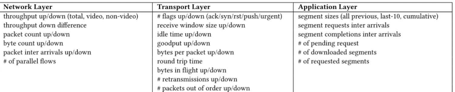
Network Layer Transport Layer Application Layer

throughput up/down (total, video, non-video) # flags up/down (ack/syn/rst/push/urgent) segment sizes (all previous, last-10, cumulative) throughput down difference receive window size up/down segment requests inter arrivals

packet count up/down idle time up/down segment completions inter arrivals byte count up/down goodput up/down # of pending request

packet inter arrivals up/down bytes per packet up/down # of downloaded segments # of parallel flows round trip time # of requested segments

bytes in flight up/down # retransmissions up/down # packets out of order up/down

Table 1: Summary of the extracted features from traffic.

3.2

Features

For each video session, we compute a set of features from the cap-tured traffic at various levels of the network stack, as summarized in Table 1. We consider a super-set of the features used in prior models [14, 25, 26] to evaluate the sub-set of input features that provides the best inference accuracy.

Network Layer. We define network-layer features as metrics that solely rely on information available from observation of a network flow (identified by the IP/port four-tuple).

Flows to video services fall into three categories: flows that carry video traffic, flows that belong to the service but transport other type of information (e.g., the structure of the web page), and all remaining traffic flows traversing to-and-from the end-host network. For each network flow corresponding to video traffic, we compute the upstream and downstream average throughput as well as average packet and byte counts per second. We also compute the difference of the average downstream throughput of video traffic between consecutive time slots. This metric captures temporal variations in video content retrieval rate. Finally, we compute the upstream and downstream average throughput for service flows not carrying video and for the total traffic.

Transport Layer. Transport-layer features include information such as end-to-end latency and packet retransmissions. These met-rics reveal possible network problems, such as presence of a lossy link in the path or a link causing high round-trip latencies between the client and the server. Unfortunately, transport metrics suffer two shortcomings. First, due to encryption, some metrics are only extractable from TCP flows and not flows that use QUIC (which is increasingly prevalent for video delivery). Second, many transport-layer features require maintaining long-running per-flow state, which is prohibitive at scale. For the metrics in Table 1, we compute summary statistics such as mean, median, maximum, minimum, standard deviation, kurtosis, and skewness.

Application Layer. Application-layer metrics include any feature related to the application data, which often provide the greatest in-sight into the performance of a video session. Encryption, however, makes it impossible to directly extract any application-level infor-mation from traffic using deep packet inspection. Fortunately, we can still derive some application-level information from encrypted traffic. For example, BUFFEST [22] showed how to identify indi-vidual video segments from the video traffic, using the times of upstream requests (i.e., packets with non-zero payload) to break down the stream of downstream packets into video segments. Our

experiments found that this method works well for both TCP and QUIC video traffic. In the case of QUIC, signaling packets have non-zero payload size, so we use a threshold for QUIC UDP payload size to distinguish upstream and downstream packets. Based on observations obtained from a dataset of YouTube QUIC sessions traffic traces, we set the threshold to 150 Bytes.

We use sequences of inferred video segment downloads to build up the feature set for the application layer. For each one of the features in Table 1 we compute the following statistics: minimum, mean, maximum, standard deviation and 50th, 75th, 85th, and 90th percentile.

4

Model Selection and Training

We describe how we gathered the inputs for the prediction model, how we selected the prediction model for startup delay and resolu-tion, and the process for training the final regressor and classifier.

4.1

Inputs and Labeled Data

Gathering input features. We train models considering different sets of input features: network-layer features (Net), transport-layer features (Tran), application-layer features (App), as well as a combi-nation of features from different layers: Net+Tran, Net+App and all layers combined (All). For each target quality metric, we train 32 models in total: (1) varying across these six features sets and (2) using six different datasets, splitting the dataset with sessions from each of the four video services—Netflix, YouTube, Amazon, and Twitch—plus two combined datasets, one with sessions from all services (which we callcomposite) and one with sessions from three out of four services (which we callexcluded). For models that rely on transport-layer features, we omit YouTube sessions over UDP as we cannot compute all features. For each target quality metric, we evaluate models using 10-fold cross-validation. We do not present the results for models based only on transport-layer or application-layer features, because the additional cost of collecting lightweight network-layer features is minimal, and these models are less accurate, in any case.

Labeling: Chrome Extension. To label these traffic traces with the appropriate video quality metrics, we developed a Chrome extension that monitors application-level information for the four services. This extension, which supports any HTML 5-based video, allowed us to assign video quality metrics to each stream as seen by the client.1

1_{We will release the extension upon publication.}

The extension collects browsing history by parsing events avail-able from the Chrome WebRequest APIs [10]. This API exposes all necessary information to identify the start and end of video sessions, as well as the HTTPS requests and responses for video segments. To collect video quality metrics, we first used the Chrome browser API to inspect the URL of every page and identify pages reproducing video for each of the video services of interest. After the extension identifies the page, collection is tailored for each service:

• Netflix: Parsing overlay text. Netflix reports video quality statistics as an overlay text on the video if the user provides a specific keystroke combination. We injected this keystroke combination but render the text invisible, which allows us to parse the reported statistics without impacting the playback experience. This information is updated once per second, so we adjusted our collection period accordingly. Netflix reports a variety of statistics. We focused on the player and buffer state information; including whether the player is playing or not, buffer levels (i.e., length of video present in the buffer), and the buffering resolution.

• YouTube: iframe API. We used the YouTube iframe API [38] to periodically extract player status information, including current video resolution, available playback buffer (in sec-onds) and current playing position. Additionally, we collect events reported by the<video> HTML5 tag, which exposes the times that the player starts or stops the video playback due to both user interaction (e.g., pressing pause) or due to lack of available content in the buffer.

• Twitch and Amazon: HTML 5 tag parsing. As the two services expose no proprietary interface, we generalized the module developed for YouTube to solely rely on the<video> HTML5 tag to collect all the required data. This approach allowed us to collect all the events described above as well as player sta-tus information, including current video resolution, available playback buffer (in seconds), and current playing position.

4.2

Training

Startup delay. We trained on features computed from the first ten seconds of each video session. We experimented with different regression methods, including: linear, ridge, SVR, decision tree regressor, and random forest regressor. We evaluate methods based on the average absolute error and conclude that random forest leads to lowest errors. We select the hyper parameters of the random forest models on the validation set using the R2 score to evaluate all combinations with exhaustive grid search.

Resolution. We trained a classifier with five classes: 240p, 360p, 480p, 720p, and 1080p. We evaluated Adaboost (as in prior work [26]), logistic regression, decision trees, and random forest. We select random forests because it again gives higher precision and recall with lower false positive rates. Similarly to the model for startup delay, we select hyper parameters using exhaustive grid search and select the parameters that maximize the F1 score. Generating and labeling traffic traces. We instrumented 11 ma-chines to generate video traffic and collect packet traces together with the data from the Chrome extension: six laptops in residences

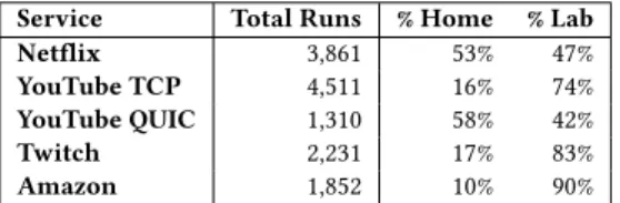
Service Total Runs % Home % Lab Netflix 3,861 53% 47% YouTube TCP 4,511 16% 74% YouTube QUIC 1,310 58% 42% Twitch 2,231 17% 83% Amazon 1,852 10% 90%

Table 2: Summary of the labeled dataset.

connected to the home WiFi network (three homes in a large Euro-pean city with download speeds of 100 Mbps, 18 Mbps, and 6 Mbps, respectively; one room in a student residence in the same city; one apartment in a university campus in the US; and one home from a rural area in the US), four laptops located in our lab connected via the local WiFi network, and one desktop connected via Ethernet to our lab network. We generated video sessions automatically using ChromeDriver[12]. We played each session for 8 to 12 minutes depending on the video length and whether there were ads at the beginning of the session (in contrast to previous work [26], we did not remove ads from the beginning of sessions in order to recreate the most realistic setting possible). For longer videos (e.g., Netflix movies), we varied the playback starting point to avoid always capturing the first portion of the video. We generate five categories of sessions: Netflix, Amazon, Twitch, YouTube TCP, and YouTube QUIC. We randomly selected Netflix and Amazon movies from the suggestions presented by each service in the catalog page. To avoid bias, we selected movies from different categories including action, comedies, TV shows, and cartoons. We ultimately selected 25 movies and TV shows used in rotation from Netflix and 15 from Amazon. Similarly for YouTube, we select 30 videos from different categories. Twitch automatically starts a live video feed when open-ing the service home page. Thus, we simply collect data from the automatically selected feed. To allow Netflix to stream 1080p con-tent on Chrome, we installed a dedicated browser extension [11]. Finally, we collected packet traces using tcpdump [35] on the net-work interface the client uses and compute traffic features presented in the previous section.

Emulating Network Conditions. In the lab environment, we manually varied the network conditions in the experiments using tc[9] to ensure that our training datasets captured a wide range of network conditions. These conditions can either be stable for the entire video session or vary at random time intervals. We var-ied capacity from 50 kbps to 30 Mbps, and introduced loss rates between 0% and 1% and additional latency between 0 ms and 30 ms. All experiments within homes ran with no other modifications of network conditions to emulate realistic home network conditions. Measurement period. We collected data from November 20, 2017 to May 3, 2019. We filtered any session that experienced playing errors during the execution. For example, we noticed that when encountering particularly challenging video conditions (e.g., 50 kbps download speeds), Netflix’s player simply stops and shows an error instead of stalling and waiting for the connectivity to return to playable conditions. Hence, we removed all sessions that required more than a high threshold,i.e., 30 seconds, to start reproducing the video. The resulting dataset contains 13,765 video sessions from Netflix, Amazon, Twitch, and YouTube, that we use to train and 5

10

₁₀

_{0 10}

₁₀

Startup Error in seconds (Real - Detected)

0.0

0.5

PDF of Errors

Net, RMSE: 1.4

Net+Tran, RMSE: 1.39

Net+App, RMSE: 1.2

All, RMSE: 1.21

Figure 2: Startup delay inference error across different features sets.

test our inference models.2Table 2 shows the number of the runs per video service and under the different network conditions.

5

Model Validation

We evaluate the accuracy of models relying on different features sets for predicting startup delay and resolution. Our results show that models that rely on network- and application-layer features out-perform models that rely on network- and transport-layer features across all services. This result is in contrast with prior work [14, 26], which provided models that rely on transport-layer features.

We also evaluate whether our models are general. A composite model—where we train the model with data from multiple services and later predict quality of any video service—is ideal as it removes the requirement to collect data with ground truth for a large number of services. Our evaluation of acomposite model trained with data from the four video services shows that it performs nearly as well as specific models that rely only on sessions from a single service across both quality metrics. This result raises hopes that the composite model can generalize to a wide variety of video streaming services. When we train models using a subset of the services and evaluate it against the left out one (excluded models), however, the accuracy of both startup delay and resolution models degrades significantly, rendering the models unusable. This result highlights that although our modeling method is general in that it achieves good accuracy across four video services, the training set used to infer quality metrics should include all services that one aims to do prediction for.

5.1

Startup Delay

To predict startup delay, we train one random forest regressor for each features set and service combination. We study the magnitude of the inference errors in our model prediction. Figure 2 presents the error of startup delay inference across the four services for different features sets. Interestingly, our results show that the model using a combination of features from network and application layer yields the highest precision, minimizing the root mean square error (RMSE) across the four services. These results also show that we can exclude Net+Tran models, because Net+App models have consistently smaller errors. ISPs may ultimately choose a model that uses only network-layer features, which rely on features that are readily available in many monitoring systems for a small decrease in inference accuracy.

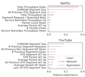
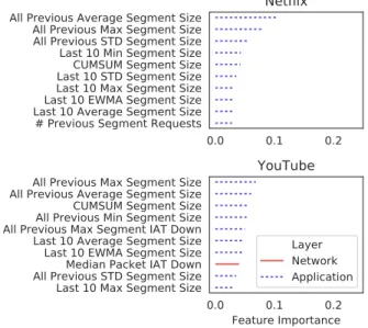
To further understand the effect of different types of features on the models, we study feature importance (based on the Gini index [8]) across the different services. Figure 3 ranks the ten most

2_{We will release the collected dataset upon publication.}

0.0

0.2

0.4

Total Throughput Down

CUMSUM Segment Size

All Previous STD Segment Size

Total Throughput Up

Segment Request / Download Ratio

_{Service NonVideo Throughput Up}

Packet Count Down

Average Packet IAT Up

_{# Parallel Flows}

Service NonVideo Throughput Down

Netflix

0.0

0.2

0.4

Feature Importance

CUMSUM Segment Size

# Previous Segment Requests

All Previous Max Segment IAT Down

# Previous Segments Down

_{STD Segment IAT Up}

STD Packet IAT Up

Average Packet IAT Up

All Previous STD Segment IAT Up

Average Packet IAT Down

Last 10 STD Segment Size

YouTube

Layer

Network

Application

Figure 3: Startup delay feature importance for Netflix and YouTube Net+App models.

important features for both Netflix and YouTube for the Net+App model. Overall, application-layer features dominate YouTube’s rank-ing with predominantly features that indicate how fast the client downloads segments, such as the cumulative segment size and their interarrival times. We observe the same trend for Amazon and Twitch. In contrast, the total amount of downstream traffic (a network-layer feature) dominates Netflix’s list. Although this result seems to suggest a possible difference across services, this feature also indicates the number of segments being downloaded. In fact, all of these features align with the expected DASH video streaming behavior: the video startup delay represents the time for filling the client-side buffer to a certain threshold for the playback to begin. Hence, the faster the client reaches this threshold (by downloading segments quickly), the lower the startup delay will be.

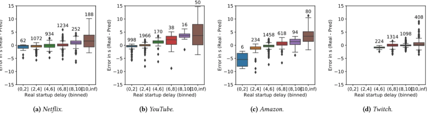
Finally, we aim to understand how much the larger errors ob-served in Figure 2 could negatively impact real world applications of the model for the different services. Figure 4 shows for each service the distribution of the relative errors for inferred startup delays split into two-second bins (using the Net+App features set). We see that the errors depend heavily on the number of samples in each bin (displayed at the top of each box): the larger the number of samples, the smaller the errors. This result is expected as the model better learns the behavior of video services with more data points, and is also reassuring as the model is more accurate for the cases that one will more likely encounter in practice. The bins with more samples have less than one second error most of the time. For example, the vast majority of startup delays for YouTube occur in the zero to four seconds bins (91% of total sample) and errors are within one second for the majority of these instances. Overall, our models perform particularly well for startup delays of less than ten seconds with errors mostly within one second (with the exception of Amazon, which only has six samples in the (0,2] range of startup 6

(0,2] (2,4] (4,6] (6,8](8,10](10,inf) Real startup delay (binned) 15 10 5 0 5 10 15

Error in s (Real - Pred)

62 1072 934 1234 252

188

(a) Netflix.

(0,2] (2,4] (4,6] (6,8](8,10](10,inf) Real startup delay (binned) 15 10 5 0 5 10 15

Error in s (Real - Pred)

998 1966170 38 16

50

(b) YouTube.

(0,2] (2,4] (4,6] (6,8](8,10](10,inf) Real startup delay (binned) 15 10 5 0 5 10 15

Error in s (Real - Pred)

6 234

1458 618 94 80

(c) Amazon.

(0,2] (2,4] (4,6] (6,8](8,10](10,inf) Real startup delay (binned) 15 10 5 0 5 10 15

Error in s (Real - Pred)

2241314 1098 408

(d) Twitch. Figure 4: Startup delay inference error across different services for Net+App specific models.

101 ₁₀0 _{0 10}0 ₁₀1

Startup Error in seconds (Real - Detected) 0.0 0.2 0.4 0.6 PDF of Errors Specific, RMSE: 1.24 Composite, RMSE: 1.45 Excluded, RMSE: 2.85

Figure 5: Relative error in startup delay inference with same or composite Net+App models.

delay). Above ten seconds the precision degrades due to the lower number of samples.

Composite models. We evaluate a composite model for inferring startup delay across multiple services. Figure 5 reports startup delay inference errors for Netflix for the model trained using solely Netflix sessions (specific model), the one using data from all four services (composite model), and finally the one using only the other three services (excluded model). The composite model is helpful in that we can perform training and parameter tuning once across all the services and deploy a single model online for a small loss in accuracy. We present results for Netflix, but the conclusions were similar for the other three services. The composite model performs almost as well as the specific model obtained from tailored training of a regressor for Netflix; the RMSE of the specific model is 1.24 and that of the composite model is 1.45. Our analysis of the data shows that errors are mostly within one second for startup delays between two and ten seconds, the biggest discrepancies occur for delays below two and above ten seconds due to the low number of samples. In summary, these results suggest it is possible to predict startup delay with a composite model across multiple services. Applying a composite model to new services. Given that all the video streaming services use DASH, our hope was to train the model with data from a few services and later use it for other services not present in the training set. To test the generality of the model, we evaluate a model for inferring startup delay, where we train with Amazon, YouTube, and Twitch data and test with Netflix (excluded model). Unfortunately, the results in Figure 5 show that the excluded model performs very poorly compared to both the specific and composite models more than doubling the RMSE to 2.91. To better

0 50 Total down throughput (mbps) 0.00

0.02 0.04

PDF

Netflix

(a) Total down throughput.

0 50 100 Num downloaded chunks 0.00

0.01 0.02

PDF

Amazon

(b) Number of downloaded segments. Figure 6: Total down throughput is similar across services; number of dow-naloded segments is not.

understand this result, we analyze the differences and similarities of the values of input features among the four different services. Although Netflix’s behavior is often similar to that of Amazon, the similarities are concentrated on only a sub-set of the features in our models. For example, Figure 6a shows the distribution of the total downstream throughput in the first ten seconds and Figure 6b shows the number of downloaded segments—two of the most important features for Netflix’s inference. We observe that the distribution of the downstream throughput is fairly similar between Netflix and Amazon. On the other hand, the distributions of the number of downloaded segments present significant differences peaking respectively at 25 and 100 segments. Given these discrepancies, the models have little basis to predict startup delay for Netflix when trained with only the other three services. Whether it is possible to build a general model to infer startup delay across services is an interesting question that deserves further investigation. In the rest of this paper, we rely on the composite models based on the Net+App features to infer startup delay across services.

5.2

Resolution

Next, we explore resolution inference. We divide each video ses-sion into ten-second time intervals and conduct the inference on each time bin. We train one random forest multi-class classifier for each service features set and service combination. Similarly to the previous section, we present aggregated results for the different layers across the studied services. We report the receiver operating characteristic (Figure 7a) and precision-recall (Figure 7b) curves for the models weighted average across the different resolution labels 7

0.0

0.2

0.4

0.6

0.8

1.0

False Positive Rate

0.0

0.5

1.0

True Positive Rate

Net Mean ROC (AUC = 0.96 ± 0.02) Net+Tran Mean ROC (AUC = 0.97 ± 0.02) Net+App Mean ROC (AUC = 0.99 ± 0.01) All Mean ROC (AUC = 0.99 ± 0.01)

(a) ROC.

0.0

0.2

0.4

0.6

0.8

1.0

Recall

0.0

0.5

1.0

Precision

Net P/R curve (AP = 0.88) Net+Tran P/R curve (AP = 0.90) Net+App P/R curve (AP = 0.96) All P/R curve (AP = 0.96)

(b) Precision-recall.

Figure 7: Resolution inference using different features sets (For all four video services).

0.0

0.1

0.2

All Previous Average Segment Size

All Previous Max Segment Size

_{All Previous STD Segment Size}

Last 10 Min Segment Size

CUMSUM Segment Size

Last 10 STD Segment Size

Last 10 Max Segment Size

Last 10 EWMA Segment Size

Last 10 Average Segment Size

_{# Previous Segment Requests}

Netflix

0.0

0.1

0.2

Feature Importance

All Previous Max Segment Size

All Previous Average Segment Size

_{CUMSUM Segment Size}

All Previous Min Segment Size

All Previous Max Segment IAT Down

_{Last 10 Average Segment Size}

Last 10 EWMA Segment Size

Median Packet IAT Down

All Previous STD Segment Size

Last 10 Max Segment Size

YouTube

Layer

Network

Application

Figure 8: Resolution inference feature importance for Netflix and YouTube Net+App models.

to illustrate the performance of the classifier for different values of the detection threshold. The models trained with application layer features consistently achieve the best performance with both precision and recall reaching 91% for a 4% false positive rate. Any model not including application features reduces precision by at least 8%, while also doubling the false-positive rate.

We next investigate the relative importance of features in the Net+App model. Figure 8 reports the results for YouTube and Net-flix, which show that most features are related to segment size. The

0.0

0.2

0.4

0.6

0.8

1.0

False Positive Rate

0.0

0.5

1.0

True Positive Rate

Netflix Mean ROC (AUC = 0.98 ± 0.00) YouTube Mean ROC (AUC = 0.99 ± 0.00) Amazon Mean ROC (AUC = 0.98 ± 0.00) Twitch Mean ROC (AUC = 0.99 ± 0.00)

(a) ROC.

0.0

0.2

0.4

0.6

0.8

1.0

Recall

0.0

0.5

1.0

Precision

Netflix P/R curve (AP = 0.93) YouTube P/R curve (AP = 0.98) Amazon P/R curve (AP = 0.95) Twitch P/R curve (AP = 0.98)

(b) Precision-recall.

Figure 9: Resolution inference across services (with Net+App features set).

4 2 0 2 4

Resolution Level Error (Real - Detected) 0.00 0.25 0.50 0.75 1.00 PDF of Errors NF (14.21 % of total)

YT (4.49 % of total) TW (5.63 % of total)AM (10.17 % of total)

Figure 10: Kernel Density Estimation function for the relative error in resolu-tion inference for Net+App models (normalized to levels).

same applies to the other services. This result confirms the general intuition: given similar content, higher resolution implies more pixels-per-inch, thereby requiring more data to be delivered per video segment. Models trained with network and transport layer features infer resolution by relying on attributes related to byte count, packet count, bytes per packet, bytes in flight, and through-put. Without segment-related features, these models achieve com-paratively lower precision and recall.

Figure 9 presents the accuracy for each video service using the specific model. We see that overall the precision and recall are above 81% and false positive rate below 12% across all services. The accuracy of the resolution inference model is particularly high for YouTube and Twitch with average precision of 0.98 for both services. The accuracy is slightly lower for Amazon and Netflix, because these services change the resolution more frequently to adapt to playing conditions, whereas YouTube and Twitch often stick to a single, often lower, resolution.

0.0

0.2

0.4

0.6

0.8

1.0

False Positive Rate

0.0

0.5

1.0

True Positive Rate

Specific Mean ROC (AUC = 0.98 ± 0.00)

Composite Mean ROC (AUC = 0.99 ± 0.00)

Excluded Mean ROC (AUC = 0.68) (a) ROC.

0.0

0.2

0.4

0.6

0.8

1.0

Recall

0.0

0.5

1.0

Precision

Specific P/R curve (AP = 0.93) Composite P/R curve (AP = 0.92) Excluded P/R curve (AP = 0.28)

(b) Precision-recall.

Figure 11: Composite vs. specific Net+App models performance for resolution inference.

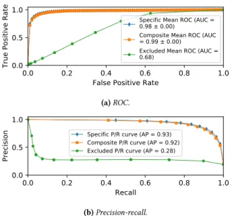
We also quantify the error rate for resolution inference. Figure 10 shows the kernel density estimation obtained plotting relative er-rors for the time slots for which the model infers an incorrect resolution. Recall that we model resolution using a multi-class classifier, resulting in discrete resolution “steps”. Hence, the error corresponds to distance in terms of the number of steps away from the correct resolution. As with the startup delay, errors tend to be centered around the real value, with the vast majority of errors falling within one or two resolution steps away from the ground truth. For example, Netflix is the service with the higher number of incorrectly inferred time slots at 14%, but 83.9% of these errors are only one step away. Even given these error rates, this model still offers a better approximation of actual video resolution than previous models that only reflect coarse quality (e.g., good vs. bad). Composite models. Figure 11 shows model accuracy when test-ing with Netflix ustest-ing the specific model, the composite model, and the excluded model. We illustrate with results for Netflix, but the conclusions are similar when doing this analysis for the other three services. The composite model performs nearly as well as the specific model (with average precision 0.92 compared to 0.93 for the specific model). These results are aligned with the general correlation between segment sizes and resolution that we observed for all services. Indeed, the four most important features for the composite model are all related to segment size: weighted aver-age and standard deviation of the sizes of the last ten downloaded segments, and the maximum and average segment sizes. This ob-servation thus provides a solid basis for a composite model based on features related to segments.

Applying a composite model to new services. Figure 11 also presents the accuracy of the excluded model, which is trained with data from Amazon, YouTube, and Twitch and tested with Netflix. As with the startup delay model, we observe a strong degradation of model accuracy in this case. The average precision is only 0.2.

0 1 2 3 Avg Previous Segment Sizes (MB) 0

2

PDF

Netflix

(a) Average previous segment sizes.

0 10 20 Max Previous Segment Sizes (MB) 0.0

0.5 1.0

PDF

Amazon

(b) Max size previous segments. Figure 12: Both max previous segment size and average previous segment size differ across services.

Our analysis of the distributions of values of the most important input features for the different services reveals even worse trends than discussed for the startup delay. Although Netflix’s behavior is most similar to Amazon’s, there are sharp differences across all the most important features. For example, Figure 12 shows the distribution for the two most important features for Netflix, the average segment size of previously downloaded segments and their max size. As a result, the accuracy of the excluded model suffers. Our comprehensive analysis of the distributions of feature values across all services indicates that achieving a general model for resolution seems even more challenging than for startup delay as services’ behavior vary substantially. As for startup delay, the rest of this paper will rely on the composite model with Net+App features to infer resolution across services.

6

Video Quality Inference in Practice

We apply our models to network traffic collected from a year-long data collection effort in 66 homes. In this section we present the chal-lenges we discovered when applying the methods in practice and techniques we apply to mitigate them. We then use the Net+App, unified models from Section 4 to infer startup delay and resolu-tion on all video sessions collected throughout the lifetime of the deployment (Table 3).

6.1

In-Home Deployment Dataset

Embedded home network monitoring system. We have devel-oped a network monitoring system that collects the features shown in Table 1. Our current deployment has been tested extensively on both Raspberry Pi and Odroid platforms connected within volun-teers’ homes. The system is flexible and can operate in a variety of configurations: our current setup involves either setting the home gateway into bridge mode and placing the device in between the gateway and the user’s access point, or deploying the device as a passive monitoring device on a span port on the user’s home network gateway. We present the software architecture and design in a separate paper currently under submission [4].

The system collects network and application features aggregated across five-second intervals. For each interval, we report average statistics for network features divided per flow, together with the list of downloaded video segments. Every hour, the system uploads the collected statistics to a remote server. To validate the results produced by the model, we instrument the extension presented in Section 4.1 in five homes. Through the extension we collect ground 9

Speed Homes Devices # Video Sessions

[mbps] Netflix YouTube Amazon Twitch (0,50] 20 329 21,774 65,448 2,612 2,584 (50,100] 23 288 11,788 50,178 3,273 3,345 (100,500] 19 277 13,201 38,691 2,030 197 (500,1000] 4 38 523 442 86 1 Total 66 932 47,286 154,759 8,001 6,127

Table 3: Number of video sessions per speed tier.

0

2

4

6

8

10

Startup Inference Error (s)

0.00

0.25

0.50

0.75

1.00

CDF

Figure 13: Effect of domain adaptation on startup delay inference.

truth data for 2,347 streaming sessions for the four services used to train the models.

Video sessions from 66 homes. We analyze data collected be-tween January 23, 2018, and March 12, 2019. We concluded the data collection in May 2019, at which point we had 60 devices in homes in the United States participating in our study, and an additional 6 devices deployed in France. Downstream throughputs from these networks ranged from 18 Mbps to 1 Gbps. During the duration of the deployment, we have recorded a total of 216,173 video sessions from four major video service providers: Netflix, YouTube, Amazon, and Twitch. Table 3 presents an overview of the deployment, in-cluding the total number of video sessions collected for each video service provider grouped by the homes’ Internet speed (as per the users’ contract with their ISP) and the number of unique device MAC addresses seen in the home networks.

Additionally, we periodically (four times per day) record the Internet capacity using active throughput measurements (e.g., speed tests) from the embedded system. We collect this information to understand relationships between access link capacity and video QoE metrics.

6.2

Practical Challenges for Robust Models

Testing our models in a long-running deployment raises a new set of challenges that are not faced by offline models that operate on curated traces in controlled lab settings. Two factors, in particular, affected the accuracy of the models: (1) the granularity of training data versus what is practical to collect in an operational system; and (2) the challenge of accurately detecting the start and end of a video session in the presence of unrelated cross-traffic.

Granularity and timing of traffic measurements. An opera-tional monitoring system cannot export information about each individual packet. It is hence common to report traffic statics in fixed time intervals or time bins (e.g., SNMP or Netflow polling intervals). The training data that we and prior work collect has a

Net + App Domain adaptation Precision Recall FPR Precision Recall FPR Netflix 86% 86% 3.4% 90% 90% 2.5% YouTube 82% 82% 4.4% 78% 78% 5.5% Twitch 82% 82% 4.6% 91% 91% 2.2% Amazon 76% 76% 6% 78% 78% 5.6%

Table 4: Effect of domain adaptation on resolution inference.

0 100 200 300 400

Session time (seconds) 0

360 480 720

Resolution

Ground Truth Net+App Domain adaption

Figure 14: Sample session for errors with/without domain adaptation.

precise session start time, whereas the data collected from a de-ployed system will only have data collected in time intervals, where the session start time might beanywhere in that interval. This cor-responding mismatch in granularity creates a challenge for training. Furthermore, any error in estimating the start time propagates to the time bins used for inference across the entire session, resulting in a situation where the time bins in the training and deployment data sets do not correspond to one another at all.

Session detection Identifying a video session from encrypted net-work traffic is a second challenge as netnet-work traffic is noisy. First, one must identify the relatively few flows carrying traffic of a given video service out of all the haystack of flows traversing a typical net-work monitor. Second, not all flows of a video service carries video. For example, some flows may carry the elements that compose the webpage where users can browse videos and others may carry ads. Finally, within the video flows, one must be able to identify when each video session starts and ends.

To detect session start and end times, we extend the method from Dimopouloset al. [14], which identifies a spike in traffic to specific YouTube domains to determine the start of a video session and a silent period to indicate the end of a video session. We evaluate their method with our ground truth and find that the session start time error typically falls between zero and five seconds due to the granularity of the monitoring system, but in some cases—because browsing a video catalog sometimes initiates the playback of a movie trailer, for example—the method may incorrectly inflate the length of any particular video session. We present further validation in [4].

Domain adaptation. Intuitively, our approach to address these challenges involves accounting for additional noise that the practi-cal monitoring introduces that is not present in a lab setting or in the training data. To do so, we introduce noise into the training data so that the training data more closely resembles the data collected from deployment. The techniques that we apply are grounded in the general theory of domain adaptation [34]; they work as follows: Because the actual start time can fall anywhere within the five-second interval, we pre-processed our training data and artificially adjusted each session start time over a window of -5 seconds to +5 10

(0,50] (50,100] (100,500] (500,1000] Speed tiers (mbps) 5 10 15 20

Startup Delay (in seconds)

(a) Netflix. (0,50] (50,100] (100,500] (500,1000] Speed tiers (mbps) 0 5 10 15

Startup Delay (in seconds)

(b) YouTube. (0,50] (50,100] (100,500] (500,1000] Speed tiers (mbps) 5 10 15

Startup Delay (in seconds)

(c) Amazon. (0,50] (50,100] (100,500] (500,1000] Speed tiers (mbps) 5 10 15

Startup Delay (in seconds)

(d) Twitch. Figure 15: Startup Delay Inference vs. Nominal Speed Tier.

(0,50] (50,100] (100,500] (500,1000] Speed tiers (mbps) 5 10 15 20

Startup Delay (in seconds)

(a) Netflix. (0,50] (50,100] (100,500] (500,1000] Speed tiers (mbps) 0 5 10 15

Startup Delay (in seconds)

(b) YouTube. (0,50] (50,100] (100,500] (500,1000] Speed tiers (mbps) 5 10 15

Startup Delay (in seconds)

(c) Amazon. (0,50] (50,100] (100,500] (500,1000] Speed tiers (mbps) 5 10 15

Startup Delay (in seconds)

(d) Twitch. Figure 16: Startup Delay Inference vs. Active Throughput Measurements (95th Percentile).

(0,50] (50,100] (100,500] (500,1000] Speed tier (mbps) 0 20 40 60 80 100 Experienced Resolution % 240 360 480 720 1080 (a) Netflix. (0,50] (50,100] (100,500] (500,1000] Speed tier (mbps) 0 20 40 60 80 100 Experienced Resolution % 240 360 480 720 1080 (b) YouTube. (0,50] (50,100] (100,500] (500,1000] Speed tier (mbps) 0 20 40 60 80 100 Experienced Resolution % 240 360 480 720 1080 (c) Amazon. (0,50] (50,100] (100,500] (500,1000] Speed tier (mbps) 0 20 40 60 80 100 Experienced Resolution % 240 360 480 720 1080 (d) Twitch. Figure 17: Resolution vs Nominal Speed Tier

(0,50] (50,100] (100,500] (500,1000] Speed tier (mbps) 0 20 40 60 80 100 Experienced Resolution % 240 360 480 720 1080 (a) Netflix. (0,50] (50,100] (100,500] (500,1000] Speed tier (mbps) 0 20 40 60 80 100 Experienced Resolution % 240 360 480 720 1080 (b) YouTube. (0,50] (50,100] (100,500] (500,1000] Speed tier (mbps) 0 20 40 60 80 100 Experienced Resolution % 240 360 480 720 1080 (c) Amazon. (0,50] (50,100] (100,500] (500,1000] Speed tier (mbps) 0 20 40 60 80 100 Experienced Resolution % 240 360 480 720 1080 (d) Twitch. Figure 18: Resolution vs. Active Throughput Measurements (95th Percentile).

seconds from the actual start value in increments of 0.5 seconds. For each new artificial start time, we recalculated all metrics based on this value for the entire session. This technique has two benefits: it makes the model more robust to noise, and it increases the volume of training data.

Validation. We validated the domain-adapted models against 2,347 sessions collected across five homes of the deployment. We com-pared each session collected from the extension with the closest session detected in the deployment data. We present results for both startup delay and resolution using the Net+App, unified model (as presented in Section 4) and the model after domain adaptation.

Figure 13 shows the resulting improvement in startup infer-ence when we apply domain adaption based models to Netflix and YouTube: In both cases, the root mean square error improves—quite significantly for YouTube. Table 4 shows that we obtain similar

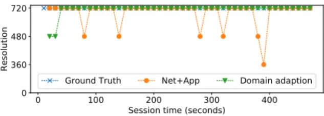
improvements for resolution inference, except for YouTube. We posit that this result is attributable to the ground truth dataset col-lected; the YouTube data is heavily biased towards 360p resolutions (90+%), whereas all other services operated at higher (and more diverse) resolutions. While domain adaptation increases balance across classes, it may slightly impact classes with more prevalence in the training dataset. We leave investigation into mitigating such issues for future exploration. Finally, Figure 14 illustrates how do-main adaption helps correct errors on resolution inference through an example session. These results suggest that domain adaptation is a promising approach for bridging the gap between lab-trained models and real network deployments. We expect that results could be further improved by applying domain adaptation with smaller time intervals.

6.3

Inference Results

We ran the quality inference models from Section 4 on all video ses-sions collected throughout the lifetime of the deployment (Table 3).

6.3.1 Startup Delay We infer the startup delay for each video ses-sion in the deployment dataset in order to pose a question that both ISPs and customers may ask: how does access link capacity relate to startup delay? Answering this question allows us to understand the tangible benefits of paying for higher access capacity with regard to video streaming. We employ two metrics of “capacity”: the nominal download subscription speed that users reported for each home, and the 95th percentile of active throughput measurements that we collected from the embedded in-home devices. Figure 15 presents box plots of startup delay versus nominal speeds, whereas Figure 16 presents startup delay versus the 95th percentile of throughput mea-surements. Note that the number of samples for the highest tier for both Amazon and Twitch is too small to draw conclusions see Table 3), so we focus on results in the first three tiers for these services.

Figure 15 shows our unexpected result. We see that median startup delays for each service tend to be similar across the subscrip-tion tiers. For example, YouTube consistently achieves a median of <5 second startup delay across all tiers and Amazon a constant me-dian startup delay of <6 seconds. Netflix and Twitch’s startup delay differs by at most ± 2 seconds across tiers, but these plots exhibit no trend of decreasing startup delay as nominal speeds increases as one would expect. There are several possible explanations for this result. One possibility is that actual speeds vary considerably over time due to variations in available capacity along end-to-end paths due (for example) to diurnal traffic demands.

Startup delays follow a more expected pattern when we consider capacity as defined by active throughput measurements. Figure 16 shows that startup delay decreases as measured throughput in-creases for Netflix, YouTube, and Twitch. For Netflix, the difference in startup delay between the highest and lowest tier is four seconds, this difference is three seconds for YouTube. This figure also high-lights the difference in startup delay across services, given similar network conditions. These differences reflect the fact that different services select different design tradeoffs that best fit their business model and content. For example, Netflix has the highest startup delay of all the services. Because Netflix content is mostly movies and long-form television shows—which are relatively long—having higher startup delays may be more acceptable. As we see in the next section, our inference reflects the expected trends that Netflix trades off higher startup delay to achieve higher resolution video streams.

6.3.2 Resolution Next, we infer the resolution for each ten-second bin of a video session. As with our startup delay analysis, we study the correlation between resolution and access capacity. For this analysis, we omit the first 60 seconds of video sessions, since many Adaptive Bitrate (ABR) algorithms begin with a low resolution to ramp up as they obtain a better estimate of the end-to-end through-put. Recall that our video quality inference model outputs one of five resolution classes: 240, 360, 480, 720, or 1080p.

Figure 17 presents resolution versus the nominal speed tier, whereas Figure 18 presents resolution versus the 95th percentile of

active throughput measurements. As with startup delay, we observe expected results (i.e., higher resolutions with higher capacities) with measured throughput (Figure 18); the trend is less clear for nominal speed tiers (Figure 17). Recall that the number of samples in the highest speed bar for Amazon and Twitch is small; focusing on the other three tiers shows a clear trend of increased percentage of bins with higher resolutions as capacity increases. For example, Netflix and YouTube in the highest speed tier achieve about 40% more 1080p than in the lowest speed tier. We also observe that, in general, YouTube streams at lower resolution for the same network conditions than other services.

Video resolution is dependent on more factors than simply the network conditions. First, some videos are only available in SD, and thus, will stream at 480p regardless of network conditions. Second, services tailor to the device type as a higher resolution may not be playable on all devices. We can identify the device type for some of the devices in the deployment based on the MAC address. Of 1,290,130 ten-second bins of YouTube data for which we have device types, 616,042 are associated with smartphones, indicating that device type may be a confounder.

7

Conclusion

Internet service providers increasingly need ways to infer the qual-ity of video streams from encrypted traffic, a process that involves both identifying the video sessions and segments and processing the resulting traffic to infer quality across a range of services. We build on previous work that infers video quality for specific services or in controlled settings, extending the state of the art in several ways. First, we infer startup delay and resolution delay more precisely, attempting to infer the specific values of these metrics instead of coarse-grained indicators. Second, we design a model that is robust in a deployment setting, applying techniques such as domain adap-tation to make the trained models more robust to the noise that appears in deployment, and developing new techniques to identify video sessions and segments among a mix of traffic that occurs in deployment. Third, we develop a composite model that can pre-dict quality for a range of services: YouTube, Netflix, Amazon, and Twitch. Our results show that prediction models that use a com-bination of network- and application-layer features outperforms models that rely on network- and transport-layer features, for both startup delay and resolution. Models of startup delay achieve less than one second error for most video sessions; the average preci-sion of resolution models is above 0.93. As part of our work, we generated a comprehensive labeled set with more than 13,000 video sessions for four popular video services: YouTube, Netflix, Amazon, and Twitch. Finally, we applied these models to 16 months of traffic from 66 homes to demonstrate the applicability of our model in practice, and to study the relationship between access link capacity and video quality. We found, surprisingly, that higher access speeds provide only marginal improvements to video quality, especially at higher speeds.

Our work points to several avenues for future work. First, our composite model performs poorly for services that are not in the training set; a truly general model that can predict video quality for arbitrary services remains an open problem. Second, more work remains to operationalize video quality prediction models to operate in real time.