Université de Montréal
Autornatic music classification using boosting algorithms and auditory features
par
Norman Casagrande
Département d’informatiqne et de recherche opérationnelle Faculté des arts et des sciences
Mémoire présenté à la Faculté des études supérieures en vue de l’obtention du grade de Maîtrise de Sciences (M.Sc.)
en informatique
Octobre, 2005
z
‘f
Université
(III
de Montréal
Direction des bibliothèques
AVIS
L’auteur a autorisé l’Université de Montréal à reproduire et diffuser, en totalité ou en partie, par quelque moyen que ce soit et sur quelque support que ce soit, et exclusivement à des fins non lucratives d’enseignement et de recherche, des copies de ce mémoire ou de cette thèse.
L’auteur et les coauteurs le cas échéant conservent la propriété du droit d’auteur et des droits moraux qui protègent ce document. Ni la thèse ou le mémoire, ni des extraits substantiels de ce document, ne doivent être imprimés ou autrement reproduits sans l’autorisation de l’auteur.
Afin de se conformer à la Loi canadienne sur la protection des renseignements personnels, quelques formulaires secondaires, coordonnées ou signatures intégrées au texte ont pu être enlevés de ce document. Bien que cela ait pu affecter la pagination, il n’y a aucun contenu manquant.
NOTICE
The author of this thesis or dissertation has gtanted a nonexciusive license allowing Université de Montréal to reproduce and publish the document, in part or in whole, and in any format, solely for noncommercial educationat and research purposes.
The author and co-authors if applicable tetain copyright ownership and moral rights in this document. Neither the whole thesis or dissertation, nor substantial extracts from it, may be printed or otherwise reproduced without the author’s permission.
In compliance with the Canadian Privacy Act some supporting forms, contact information or signatures may have been removed from the document. While this may affect the document page count, it does flot represent any Ioss of content from the document.
Université de Montréal Faculté des études supérieures
Ce mémoire intitulé:
Automatic music classification using boosting algorithms and auditory features
présenté par:
Normau Casagrande
a été évalué par un jury composé des personnes suivantes:
Guy Lapalme présideit-rapporteur Douglas Eck directeur de recherche Balàzs Kégl codirecteur Yoshua Beugio membre du jury
Avec l’augmeutatiou de l’accessibilité à la musique digitale, il devient de plus en plus nécessaire d’automatiser l’organisation de bases de données musicales. Actuellement, les utilisateurs organisent leur bases de données en se basant sur les méta-données des pièces musicales, telles que le nom de l’interprète, le titre de la pièce et de l’album, eu plus d’aspects plus subjectifs comme le geure musi cal et l’ambiance. Par contre, ces informations doivent normalement être ajoutées manuellement et ne sont souvent pas précises ou complètes.
Dans ce mémoire, nous présentons plusieurs techniques d’extractions de car actéristiques (“features”) de fichiers audio qui sont utiles pour la classification de pièces musicales dans certaines catégories définies par l’usager. Ces techniques utilisent des concepts la théorie de traitement de signal, de la psychoacoustique et de la perception auditive humaine.
Pour traiter la grande quantité de charactéristiques générées par notre approche, nous utilisons une version multi-classe de l’algorithme AdaBoost. Nous décrivons cet algorithme et nous le comparons avec d’autres approches. Nous présentons aussi des expériences tendant à montrer que notre méthode est plus performante que d’autres méthodes de pointe sur une collection musicale étidluetée manuellement pour la classification de genres musicaux. Nous analysons aussi la performance de notre système à la compétition internationale MIREX 2005, où notre système a terminé premier parmi les 15 soumissions.
Finalement, nous présentons une nouvelle approche pour la modélisation de la structure de la voix, utilisantune représentation visuelle de celle-ci. Nous montrons que ce modèle peut déterminer si un signal sonore correspond à de la voix ou à de la musique, et ce en utilisant une fraction des ressources CPU qui sont nécessaires aux autres approches publiées.
Keywords: AdaBoost, apprentissage machine, recherce d’information musicale, classificatoin de genres musicaux, distinction de la voix et la musique, classification multi-classe, similarité musicale
ABSTRACT
With the huge increase in the availability of digital ninsic, it has become more important to automate the task of organizing databases of musical pieces. Cur rently users have to rely on meta-information such as performer. album, titie, as
well as more subjective aspects such as genre and mooci, to arrange these clatabases or to create playlists. However, this information must be adclecl manually anci it is often inaccurate or incomplete.
In this thesis we describe how extract from the audio files features that are
meaningful for a classification into categories clefined by the user. We show how
to extract information using knowledge from signal processing theory, physics of sound, psychoacoustics, humaii auditory perception, and use it to discriminate
high-level characteristics of music, such as music genre.
To deal with the very large number of features generated by ouï approach, we use a multiclass version of the ensemble learner AdaBoost. We describe our algo rithm and compare it to other approaches. We present experimental evidence that ouï method is superior to state-of-the-art algorithms on a hand-labeled database for genre recognition, and describe ouï performance at the recent MIREX 2005 inter national contest in music information retrieval, where our algorithm was the best
genre classifier among 15 snbmissions.
We also present a novel approach to model the pattern of specific souncls (i.e. speech), using a visual representation of sound. We show how this model can successfully discriminate speech from music at the frame level, nsing a fraction of the CPU usage of other approaches.
Keywords: AdaBoost, machine learning, music information retrieval,
audio genre classification, music/speech discrimination, multi-class clas
o
CONTENTS
RÉSUMÉ iii
ABSTRACT iv
CONTENTS y
LIST 0F TABLES viii
LIST 0F FIGURES ix
NOTATION xii
DEDICATION xv
ACKNOWLEDGEMENTS xvi
CHAPTER 1: INTRODUCTION 1
1.1 Brief Iutrodrictioii to J\Iachine Learllillg 3
1.2 Structure of the Thesis 7
CHAPTER 2: CLASSIFIERS 10 2.1 Boosting 10 2.2 AclaBoost 12 2.3 Weak Learners 21 2.3.1 Decision Stumps 21 2.3.2 Decision Trees 23 2.4 Ada3oost Extensions 25 2.4.1 Abstention 25 2.4.2 Regularization 27 2.5 Multi-class AdaBoost 29 2.5.1 AdaBoost.VI1 30
vi
2.5.2 Ada3oost.MH 30
2.5.3 AdaBoost.MO 36
2.6 Other Classifiers 39
2.6.1 Support Vector Machines 39
2.6.2 Artificial Neural Networks (ANNs) 40
2.7 Conclusion 40
CHAPTER 3: AUDIO FEATURE EXTRACTION 41
3.1 Prame Level Timbrai Pentures 42
3.1.1 PFTC 43 3.1.2 RCEPS 43 3.1.3 MPCC 43 3.1.4 ZCR 44 3.1.5 Rolloif 44 3.1.6 Spectral Centroid 45 3.1.7 Spectral Spread 45 3.1.8 Autoregression (LPC) 45
3.2 Blending frame-level audio features 46
3.3 Auclitory Temporal Pentures 47
3.3.1 Autocorrelatioll 47
3.3.2 Phase Preserving Autocorrelation 49
3.4 Haar-like Pentures 53
3.4.1 Reclucing the training time 57
3.5 Conclusion 59
CHAPTER 4: EXPERIMENTS 60
4.1 Experiments on the IVINIST Database 60
4.1.1 Raw Data Experiments 61
4.1.2 Haar-Like Features 63
4.1.3 Regularization 66
c-4.1.5 Feature Selection 01) a Subset of Data 67
4.1.6 Comparison with Other Algorithms 68
4.1.7 Discussion 69
4.2 Frame Level Speech/Music Discrimination 71
4.2.1 The Algorithm 73
4.2.2 Experimental Resuits 75
4.2.3 A Winamp Plugm 78
4.2.4 Discussion 80
4.3 Music Genre Recognition 81
4.3.1 Haar-Like Features 82
4.3.2 The Segmentation Algorithm 83
4.3.3 Data Set 85 4.3.4 Acoustic Features 85 4.3.5 Classiflers 86 4.3.6 Resuits 87 4.3.7 Discussion 88 1.1 MIREX 91
1.1.1 Simulation on Tzauetakis Genre Database 92
4.4.2 Genre Classification 93 4.4.3 Artist Identification 95 4.4.4 Discussion 96 4.5 Conclusion 98 CHAPTER 5: CONCLUSION 100 5.1 Future Work 101 BIBLIOGRAPHY 104
LIST 0F TABLES
2.1 An example of ECOC decomposition matrix with a 7-bit class cod
ing. on a 4 classes problem 38
1.1 Accuracv and training time for MMST raw data 63 4.2 Accnracy ancl training time using the Haar-like features 66
4.3 Resuits with and withont abstention 67
4.4 Results by taking a snbset of the data at cadi iteration 68 4.5 Results of the Haar-hke approach compared to other algorithms on
the MNIST database 69
4.6 Testing error rate using single frame features 76 4.7 A comparison of varions freine ievel featnres 77 4.8 Tbe resnlts on the 2.3 second segments size for the Tzanetakis database,
with training and test time 94
4.9 Summarized resuits for die Genre Recoguition contest at MuREX 200.5 96 4.10 Summarized resnlts for the Artist Identification contest at MIREX
200.5 97
4.11 The results withont and with tempo on the 2.3 second segments size
1.1 An exaniple of training process 5 1.2 The overfitting explaineci using cats and dogs 6 2.1 The evolution of the weight distribution in ADABOOST over the
iterations 14
2.2 The XOR problem 23
2.3 A decision tree 24
2.4 The two different ways of treating the multiclass problem with stumps 33
2.5 A multiclass problem mapped with differeint À functions 37
3.1 The autocorrelationi of the Bine Dannbe 48
3.2 The autocorrelation of n song by Manos Xatziclakis from ISMIR 2004 50
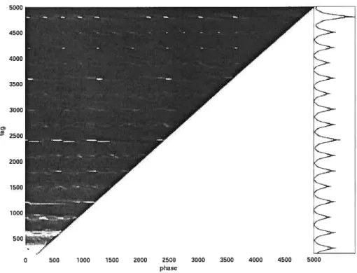
3.3 The autocorrelation phase matnix 51
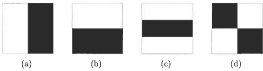
3.4 The entropy calculation of the song by Manos Xatziclakis 52 3.5 Four possible configurations of the Haar wavelets 54
3.6 The integral image value of a single point 56
3.7 The integral image value of a rectangular area 57 3.8 Two plots of the error space for the speech/music discrimination
problem 58
4.1 Trailling and test curves on raw MNIST data 62
4.2 An integral image representation of number “four” 64 4.3 The test error curve of the I\/INIST data using Haar-like features 65
4.4 The evolution of slightly changes in 6 67
4.5 The reconstruction of the ten digits using the Haar-like features
founci during training 70
4.6 The probability map of the first two types of Haar-like features 71
4.7 The spectrogram plot of speech and music 72
X
4.9 Tire discrimination power of a three-block Haar-like feature 75 4.10 Tire output of tire three-block Haar-like feature for ail training points 75 4.11 Tire resuits on a 2Onrs PET franre, without and witlr smootlring 76
4.12 A \Vinamp plugin version of our model 78
4.13 Tire segmentation of tire the song 83
4.14 Tire classification accuracy on four different feature sets 87 4.15 Tire classification accuracy of ANNs anci SVM5 for different segurent
iengtlrs 89
4.16 Tire classification accnracy on four different type of features, and ail
tire aigoritlrnrs 90
4.17 Tire perfornrance of ADABOOST witir different segnrent length 93 4.18 Tire song test-error curves of tire two weak learners on 2.3 seconds
1 Basic AdaBoost 17
2 AdaBoost with margin anci abstention 29
3 AdaBoost.I\IH 35
NOTATION
General:
R Real numbers
n Tire number 0fexamples D The training set of size n
k The number of classes
x The vector of observation for example i, wbere x1 E R’1
d The number of elements (or dimensions) of tbe observation vector, that is d = xl
x) Tbe jth element of vector x
y Tire label of example x for binary classification, where yj E {—1, 1} y Tire vector of labels, for multi-class calssification
L Tbe label index
1 if x belongs to class L —1 otherwise.
6 An arbitrary small vaine bigger than zero 1 ifx=true
E{x}
Ç
1.
0z y xis definedasy Binary AdaBoost:
a(t) Tire confidence paranreter at iteration t, wbere n E R w Tire reai valned vector of weigirts
m Tire weigirt of exaurpie i, where m E R t Tire iteration index
h()(x) Tire hypothesis fttnction. fouird by tire weuk tearner at iteration t, where for our problems h Rd {—1. ±1}
7 Tire space of tire hypotheses (h E 7)
j(T)(X) Tire stroirg learner. defined as Œ(t)h(t)(x) wliere
f
: , Re() Tire error. ciefllled as Çt
{
11(t)(xi)#
}
y( Tire edge. defineci as 1 — 2E(t)
p Tire unnornralized fttnctionai margin of example i, cieflireci as
f(T)(x)y
Tire urisciassification rate
RL A generic (baseci on a loss fuirction L) eurpiricai risk Re Tire exponential enrpiricai risk
Z(t) Tire normaiization factor to keep tire weigirts a distribution. Is
as (t exp (_n(t)h(t)(X.)y.))
AdaBoost Extensions:
÷ Tire sum of weiglrts for correctty ciassified exampies e_ Tire suirr of weiglrts for incorrectÏy ciassifieci examples
e0 Tire sunr of weights for abstazned exanrples
9 Tire ecige offset paranreter. wliere 9 E R Decision Stumps:
q Tire tirresholci of tire eut, wlrere q E R
y Tire ahgnment value, where y E {—1, 1}
f
1 if q,j,q(x)
—1 otherwise
AdaBoost .MH:
w Tire weigirt of exairrple i aird ciass
y Tire a.hgnnrent vector, wlrere e E {—1 i}k g(x) Tire urulti-ciass strong lea.rirer. wlrere g : W1 —
xiv AdaBoost.MO:
Y
The set of the labelsH(x) The k-polichotomy that is H X —
Y
(y) The fullctionthat maps a label yhto one of the two complementary
sets f
xAy The Hamming distance between x and y Feat u r es:
u A real valued vector of length T that represent either n frame (on frame-level features) or the whole signal (on autocorrelatioll) T The length of the signal, that is T =
clct The discrete cosine transformation
F 11e discrete Fourier transformatioii (DFT) of frame u n A real valueci vector representing the autocorrelation
t The lag index
A
A real valueci matrix representing the phase autocorrelatioll ç5 The phaseS(x) The Shannon entropy of input vector x. where S : RIXI R
The integral image at point (a. y) of image
I.
clefined asz-1 z=1
ACKNOWLEDGEMENTS
I would like to thank my supervisors, Dr. Douglas Eck and Dr. Baldzs Kégi, for their help, encouragement anci support. Thanks also to James Bergstra who shared with me most of the work on genre recognition, and Dumitru Erhan for running the experiments with SVMs. Thanks to ail my friencis at the GAMME and LISA laboratories at the Université de Montréal for the wonderful times and interesting conversations.
Thanks to niy family, in particular to my mother, father and sister for support ing me ail these years. Thanks to my girifriend for the coiistant support and for keeping my motivation up in the last two years.
INTRODUCTION
In the last two clecades digital music has transformed the landscape of music distribution. Originallv developed hy Philips for its Compact Dises. this technologv with the advent of the internet has reached its true potential. Once cligitalized, a song eau be copied millions of times without ay production cost, anci through the internet immecliately clistributecl into the home of the customer. A successftil example of this revolution is the iTunesMusicStore, from Apple. which sold more
than 500 millioiis files since it was launched in 2003.
Portable MP3 players also play a key role, by eliminating the physical support that was once associated with music, allowing large databases of music (an iPod
contain up to 60 Gigabytes of data) to be carried anywhere.
This increased storage. coincideci with the parallel increase in the ways that n user eau access and purchase online music. The music store from Apple lias a catalog of more than 2 million soiigs, which is, on its own, several orclers of magnitude smaller of what is available on P2P networks. Thiswide selection is not
the result of an increase in production of music. but instead the effect of tlie two key factors that we have previously mentionecl: ease of distribution and copying.
As a result, it is becoming increasingly harder to arrange and navigate the large databases of music that are available to the user. Currently, the majority of tools for organizing music use naive grouping strategies based on meta-clata information introduced by the user or the creator. Short text fields describe the performer, composer, album, title, as well as niore subjective aspects such as genre and mood. Unfortunately this meta-data is often inaccurate or incomplete. Projects like Mu sicBrainz (mus icbrainz.org) promise to address this issue by analyzing each file
to obtain a fingerprint. which it used to querv a central database for meta-ciata. However, even assuming a complete meta-tag data. there is stili a problem with relying on a canonical set of moods or genres to be used by ail listeners. In fact,
2 although researchers have defined full taxonomies for the purpose of testing model performance (e.g. MacKay auJ Fujinaga [MFO5]), there is stiil no canonical tax onomy of record music, nor xviii there ever 5e. i\/lood has the same problem, even if some attempts have been made in the past to take advantage of it [LLZO3].
Because of these problems, building playlists or discovering new music using meta-tags is extremely hard. Ideally the user shoulci lie able to submit a set of music files (keysongs”, instead of keywords) and obtain in return a list of similar entries. This would allow the listener both to dynamicaliy build playlists using his database, anci intelligentiy explore the vast archive of music ouline.
Receritly there lias been many efforts to makes this scenario a reality. Software such as Indy (indy. tv) or ikate (irate. sourcef orge .net) rely on collaborative
filtering techniques to create playlists based on the interests of a user by collecting taste information from a network of listeners. The basic idea is that if in tire past two users have agreed, they xviii aiso tend to agree in the future. This approach allows a user to cliscover new content, but suffers from three key disadvantages. Tire first is that if the pool of users is too small in comparison to tIre number of songs, there will be songs in the user’s database that cannot lie used to draw a profile, because nobody but the user lias ever listened to them. This gives rise to the second problem: if there is n new baud which is proposing its work, it is not possible to position it in the ‘preference” space, as nobody knows anything about it yet. Finally, the preference given to a music piece may greatly vary depending on the situation. If a user hkes both Metallica auJ Mozart, it does irot necessarily mean that lie xvants to listen to them in the sanie session.
Another approach is to move the focus from tire user-eclited features to descrip tors that can lie automaticaily extracted from tire music. These types of features should be more reliable as they redluire no intervention by a set of users. A recent survey by Aucouturier auJ Pachet [APO3] gives a comprehensive list of features used for music information extraction, although research in feature-extraction con tinues.
classify into categories that match the nser’s taste. IViachine learning is a field of computer science that, roughly speaking, analyzes the data using statistical algorithms. Snch algorithms conld. for instance, create a model that discriminates the categories using a labeleci dataset as training data. This strategy has proven very successful, and has already been used in many prodncts, such as IVlusicMagic, from Predixis (predixis.biz), or Musipedia (www.musipedia.org)’.
Our contribntion in this thesis is the description of several effective feature ex traction techniques and learning algorithms that cnn be nsed to face the challenges of automatic music classification.
In this work vie are using part of the work previously pnblished by the author for the ICMC [CEKO5a] and ISMIR conferences [ECO5, CEKO5b], and of a recent submission to the Machine Learning Journal [BCE+05}.
1.1 Brief Introduction to Machine Learning
Machine learning generally refers to the area of artificial intelligence that con cerns making computer “learn” a specific pattern or task. Different learning prob lems are addressed by different familles of algorithms. There are grouped basically in this simplified taxonomy:
• Supervised learning algorithrns generate n function that maps the inpnts to desired outputs. Fo instance, in classification they are used in cases where each example bas a set of attributes and a label, and the algorithm has to find a generalization of the attributes that characterize each label.
• Unsupervised learning algorithms, on the other hand, work in situations where ouputs (or labels in classification) are not provided for training. A common task of nnsupervised learning is the automatic selection of “clusters” in the data in feature byperspace, or in a transformation of it, sucb that missing attributes cnn be inferred.
1A list ofmusic information retrieval systems is available at http: //mirsystems. in±o/index. php?id=mirsystems.
4 • Reinforcement learning algorithms, learn a policy by interacting with the world. Each action fias some impact on the environment, which returus a feedback (a reward or a penalty) that guides the learning algorithm to reflue the actions it takes in various situations.
The learning algorithms used for this work are ail supervisecl algorithms. These eau be further subdivided into two types: regression and classification algorithms. In regression, the algorithm maps an observation onto a real value. In classification the chosen labels form a closed set, and the classifier maps an observation to a label that belongs to the set. Classification algorithms are the type of learner that interests us, as we want to classify sound into discrete labels that follows a specific, though not absolute. taxonomy.
To train supervised learning algorithms, we need a training set that contains ri examples with the corresponding labels. Formally, training set D is defined as
{
(xy, p1) (x,, y)}
2 for binary problems. Each data poht corisists of an obser vation (or attributes) vectorx = (x(b, . . . , d containillg the description ofthe example, and a binary label yj {—l, 1} that telis in which class the example belongs to.
Each example can be considered as a point in the hyperspace of features; that is, each component of the observation vector is n value that defines the coordinate insicle the hyperspace. For instance if the dataset represents pets, the feature set rnight be
Pet : {Heigkt, Width, Weight, Legs, Furryness},
and each pohit deflned as a coordinate in this six dimensions space, for instance an example belonging to class cat might have this observations
X0t = {20, 40,4.3,4, 1.1}.
2Throughout this work we vi11 use uppercase symbols (e.g., A) to denote real-valued matrices, bold symbols (e.g., x) for real-valued vectors, and their italic counterparts (e.g., xj or (r)) to refer to elernents of these vectors.
In tire binary case, our examples will be labeleci either “cat” (1) or “other” (-1). Tire job of tire learnhrg aigoritirnr is to find tire paranreters witlrin itsown nrodei
(and wiricir depend on tire type of algoritirnr) by analyzing tire training set D. Tire resniting function f(x) xviii use tirese paraureters to return a binary decision on exanrpie X.
Tire classifier is assunred to be abie to predict tire correct output for exanrpies, not present in tire original training set, thns to generalize. A natnral way to evaluate tire error of tire classifier is by looking at tire nrisciassification rate, tirat is
wirere tire inclicator function E {A} is 1 if its argnirrent A is truc and O otirerwise.
C
Fignre 1.1: An exanrpie of training process, in wiricir tire training error reacires zero after sonre tinre, as tire aigoritirirr acijust itseif to nratcir very specific features of tire trahrhrg data. As resuit, tire error on a ireici—out test set hrcrease.
During iearning, tire aigoritirnr evaiuates tire exanrpies of tire training set, and as it goes on, it generaiiy iras tire training error Rtrajn going ciown. However, the iearning process nriglrt beconre too specific. For instance if tire aigoritirnr adjnst its paranreters to nratcir very specific featnres of tire training data, hke tire vaines of 20, 21, 24 for tire ireigirt of cats, it xviii perfectiy ciassify ah tire cats witir tirese
specific ciraracteristics, but not tire ones witir ireigirt 23. Tins situation is defined
overfitting
“optiniai”
--Trainjn
-6
as overfitting, anci is depicteci in Figure 1.2.
Dog? 4 )II4
)“4
c3) t>dt.
4 ii4Jj
1jL
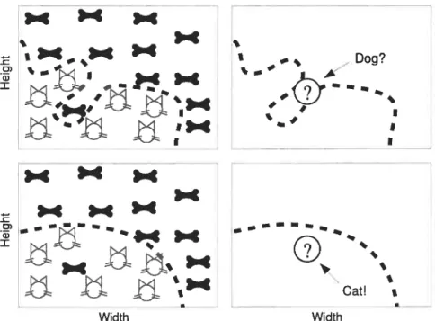
, Cat! Width WidthFigure 1.2: Cat and dogs coulci be classified just considering their size. The vast majority of cats are smaller than the vast majority of dogs; however, some clogs might be particularly small. A learning algorithm that overfits would draw an extremely complicate clecision boundary to inclucle tire single case in which the dog is very small (upper left). This bounclary will fail to classify correctly an animal, depicted by a question mark point, that is very likeiy to be a cat. A learning algorithm generalizes in the sense that it sticks more with geireral trends, rather than specific cases, as in the bottom figures.
An algorithm must be abie to obtain low error on a held-out dataset, called test set, for which the error decline as the learning process progresses, and raise when the algorithm start overfitting. Tire learning algorithm must be stopped when the model returns tire lowest test error, as showed in Figure 1.1. If this is clone before the minimum lias been reacheci, tire algorithm is ‘anderfitting. A learning algorithm is capable ofgeneralization if it can balance between overfitting and underfitting.
Often, to avoid a bias toward the test set (that is. liaving chosen the perfect parameter for the test set. which might not correspond to the optimal one in a general sense), a third set. calleci vatidation is used as stopping criterion, and the test set for evaluation.
ADABOOST algorithms, which we xviii discuss in Chapter 2 have the interesting property of being very resistant to overfitting in manv real-world problems, with a test curve that keeps decreasing eveu after the training error reaches zero.
1.2 Structure of the Thesis
We propose to use ADABOOST as a learning algoritlim to create the models for ouï classification tasks. Introduceci by freund and Schapire in 1997 [FS97], this algorithm is one of the best general purpose learning methods developed in the last decade. k lias inspired several learning theoreticai resuits and, due to its simplicity. fiexibulitv. and excellent performance on reai-worici data, it lias gained popularity ainong practitioners. Chapter 2 is mainlv declicated to clescribing this algorithm.
In Section 2.1 xve briefty go through history of this algorithm, anci in the follow— ing sections we discuss the important aspects that characterize it. its extensions, and how to implement it. In particular, in Section 2.5 we show how to extenci
ADABOOST in order to solve inultic1ass probleins, that is, probleins xvith more than two labels.
This algorithm is partictilarly interesting becanse it lias proven effective in deal
ing with the large number features that we are using. A single song can have
hundreds of feature elements. ‘vVe cali these elements dimensions because a single observation could be described as a point in a hyperspace where cadi element is a dimensjon. In snch a linge space it is very difficuit to regroup points as they “look” very sparse, unless the number of examples is very large. Tins is knoxvn as the curse of dimen.sionatity [BelGl]. With ouï experimeuts in Section 1.3 ‘e show how ADABOOST can he very competitive on these problems. as it selects and
8 aggregates only the elements of the features that are needed for the classification. I\/Iusic has a complex structure that warrants several parallel approaches. Using the simple raw signal alone is not a viable approach, for reasons relateci to psy choacoustic and computational power that we discuss in Chapter 3. Instead, we are relying on features that capture various aspects of music that are important for humans. This work is motivated by knowledge from signal processing theory, physics of sound, psychoacoustics, human auditory perception and music theory.
Li and Tzanetakis [LTO3b] define three types of auditory features: the timbral texture, the rhythm, and the pitch. Timbre is the souncl—quality of near-instants. or simply the quality of a musical sound. We present several standard techniques to extract this kind of features in Section 3.1, ancl in Section 3.2 we show how we eau blend their output together to cut down the size of the generated data, without reclucing the cua1ity of the information.
Rhythm involves the variation and duration of patterns of sounds in time. The
structures that are defined by these patterns are ultimately the essence of music. In Section 3.3 we discuss two different approaches to capture one basic component
of rhythm: musical tempo.
Finally, pitch is the psychoacoustic perception of the frequency of n sound (i.e. n note). We do not discuss pitch here because it is extremely hard to capture in polyphonic sounds, and current methods are fairly unreliable.
The last part of the chapter, Section 3.4, is dedicated to a novel approach that uses a robust image classifier to learn patterns in a visual representation of music. The basic iclea is that if music is rendered as an image, for instance using a short
discrete Fourier transformation (SDFT) that plots frequency on one axis and time on another, we cnn use simple visual features —called Haar-like features —to map
the “areas” that characterize the sound we are trying to learn. We proved the effectiveness of this technique by building a robust speech/music discriminator, discussed in Section 4.2.
In Chapter 4 we will show the resuits of experiments on the algorithm anci the features. In Section 4.1 we will evaluate the hyper-parameters of ADABOOST using
a well known database as testbed.
\‘Ve use timbrai anci rhythmical features and ADABOOST to builci a state-of the-art classifier for music genre, described in Section 4.3, and in the following section we show the resuits of MIREX 2005 international contest in music information extraction, where otir audio genre recognition algorithm ranked first in audio genre classification among 15 submissions.
CHAPTER 2
CLASSIFIERS
In this chapter we will priinarily cliscuss boosting algoritlims, and in particular ADAB00sT, which has proveci in our experiments to be very effective for solving problems related to information music retrieval.
For genre classification (see Section 4.3) we compare ADABOOST with Support Vector Machines (SVMs) and Artificial Neural Networks (ANNs), therefore we will discuss them briefly in Section 2.6. For a more complete treatment of SVMs see [HTFO1]. For a more complete treatment of ANNs see [3is95].
2.1 Boosting
There is an old saying that states “there is strength in numbers”, that is, the resuit of a group can lie higher than the simple sum of its parts. This is also, in some extent, true for machine learning.
Research in so-called ensemble learning algorithms lias been made since long time. The simplest method that uses this iclea is similar to democracy: we have a set of enperts that give an opinion on an input example. The final vote is an average over these opinions. We define our expert as a function h(x) that receives an input Xalld returns a positive or negative vote: formally {h : {—1, +i}}. The averaged learner f(x) is the resuit of the linear comhination of the functions
f(x) =
for N functions.
This is generally defined as ensemble of experts, anci it is often applied when the experts corne frorn very clifferent areas, which in machine learning can mean that the algorithms are very different. it is important to note that in the previous
equation the experts evaluate the same attributes of the same example. This might not aiways be true, as there may be experts that treat different aspects of a problem. These aspects must be correlated in some sense. or else the experts will end up forming opinions based on incompatible evidence.
Ensembles of experts are similar to the strategy of another popular algorithm caiied bagging. With bagging. also known as bootstrap agg’regation, we generate J subsets {D1, . . ,D} of data by sampling from a training set D. We then learn n
moclel on each subset, and finally combine the models by averaging the output (in the case of regression), or voting (in the case of classification).
This method is often usecl with n single algorithm repeated many times, instead of n number of clifferent algorithms, and it reduces variance and generally helps to avoid over-fitting. The subsets D can also have the saine size of D, and in this case ail exampies will be repeateci in each D.
Schapire [Sch9O] did n further deveiopment of this idea, defined as boosting, which was the first simple procedure in the PAC-learning framework theorized in 1984 by Valiant [Va184]. In Valiant’s model the notion of successful learning is formally defined using probability theory. A learner is said to have accuracy (1—E)
with reÏiabiÏity (1—6) if it generates a binary hypothesis whose accuracy is at least
(1 — E) with probability at least (1 — 6), where c is the error of the learner, and 6
is a parameter which defines the confidence. The probability that the algorithm fails is measured with respect to n ranclom choice of exampies given in the learning algorithm and in n possible internal randomization of the algorithm. Very roughly speaking, the learner gets samples that are classified according to a function from n certain ciass. The aim of the learner is to find an arbitrary approximation of the function with high probability.
Schapire showed that a learner, even if rough and moderately inaccurate, could always improve its performance by training two additionai classifiers on filtered version of the input data stream. These algorithms, are cailed ‘weak tea’rners be cause their performance is guaranteed (with high probability) to be only slightly better than chance. After learning an initial classifier h’ on the first n training
12 points,
• Ïi(2) is lea.rned ou a new sample ofn points, haif of winch are misclassified by
• W3) leariied on n points from which h’ aj (2) disagree. • the boosted classifier is h) = MAJORITYVOTE(h(1), h12, k(3))
Schapire’s “Strength of Weak Learnability” theorem proves that lias improved performance over
‘vVith a number of learners larger than three, the algorithm is defined redur sively. Each level of the recursion is a learner whose performance is better than the performance of the previous recursion level. The final hypothesis generated can be represented as a circuit consisting of many three-input majority gates.
In 1995 Freund [Fre95] proposed a “Boost by Majority” variation which coin bineci manv weak learners simultaneousl in a single tayer circuit, and improved the performance of the simple boosting algorithm of Schapire. The improvement is achieved by combining a large number of hypotheses. each of which is generated hy training the given learning algorithm on a clifferent set of examples.
The biggest weakiress of this algorithm is f lie assumption that each hvpothesis lias n fixeci error rate, anci is therefore difficuit to use in practice.
2.2 AdaBoost
Illtroduced in 1997 by Freund and Schapire [FS97], the ADABOOST algorithm
solved many of the practical difficulties of the previous boosting algorithms. Un like the previous boosting algorithms, ADABOOST needs no prior knowledge of the accuracies of the weak hypotheses. Rather, it adapts to these accuracies and generates a confidence parameter n that changes at each iteration according to the error of the weak hvpothesis. This is the basis of its naine: Ada’ is short for
For this section we assume the binary case. Tiierefore we have an input training set D = {(xi, yi) (x, yn)} where each label yj E -(—1,
+1}.
The algorithm(t) (t) (t)
mantains a weight distribution w = (w1 , . . . ,w,
)
over the data points. Ingeneral. the weight îu xviii express how hard it is to classify x.
The basic ADABOOST algorithm is remarkably simple. In a series of rounds or iterations t = 1 T a weak learner WEAK(D. w) fincis a binary weak hypothesis
(or base classifier) h. coming from a subset fl of {h : — {—1, +i}} appropriate
for the distribution of weights w(t), that is xvith the Ïoxvest weighted error. When this is not possible, a subset of the training examples can be sampled according to w(t) (for instance with a stratified sampling of the xveights which takes the hardest examples with higher probabihty), anci these (unweighted) resampled examples can be used to train the xveak learner.
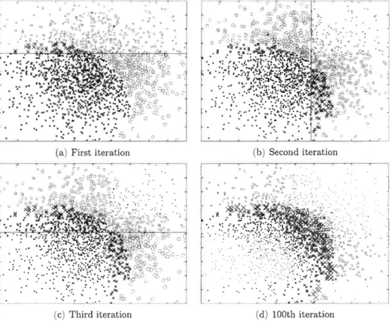
At the beginning. the weight vector is initiahzed to be equai for each point. On each boosting round. the weight of incorrect examples is increased so that the weak iearner is forceci to focus on the hard exampies on the training set. Figure 2.1 shows the evoiution of this distribution on a simple two climensional problem and a Decision Stumps weak learner (which we xviii sec in Section 2.3).
Formaily the goal of tue base classifier is to minimize the weighted error at iteration t
(t) = c(t)(h) w{h(t)(x)
#
yi}, (2.1)This is eciuivaient to maximizing the edge
(t)
1 — 2E(t)
=
m(t)11(t)(Xj)yj.
Freund and Schapire proved that for the binary case the error of the final hypothesis (xvith respect to the observations) is bounded b exp (—2 7(t)2). Since a weak hypothesis that makes an entireiy random gttess has error 1/2, 7(t) ineasures the
accuracy of the tth weak hypothesis relative to random guessing. The important consequence is that if we can consistently find xveak hypotheses that are slightly
14
ta) First iteration
L. Z.)i
‘t,
‘
(e) Thirt I ittrtt ion
(b) Second iteration
s
(d) ]OOth iteration
Figure 2.1: ADABOOST mantains a distribution of weights w on the examples, as showed by the size of the points. The four images represent the state of the weights after the first, second, third and lOOth iteration. After 100 iterations it is clear how the weight focuses the attention of the weak learner on the hard examples near the boundary of the two classes. The first three figures show the threshold position of the weak learner used: a decision stump described in section 2.3.1.
e, ‘t,,,. r., .“,“‘,‘“d; c e o o o e, o o -° o -°‘e :“ O 0’ ‘c. , , , .. . et ____________
better than coin flip. the training error of the final boosteci classifier will drop
exponentiatÏy jast.
A significant clifference with the previous boosting algorithm is that the bound
011the accuracy of the final hypothesis improves when
any
of the weak hvpotheses isimproved, where previously the performance bound dependeci only on the accuracy of the last accurate weak hypothesis. On the other hand if the weak hypotheses have the sanie accuracy, the performance of ADABOOST is very close to that achieved by the best of the prececling boosting algorithms.
Once the weak hypothesis h(t) lias been receiveci, ADABOOST chooses a coeffi cient a() that measures the confidence assigned to h(t) anci it is directly related to its error
(t) 1 /1 +7 1 (1—
ln
(t)] = 1n (t)
)
(2.2)Note that () > O because c(t) < 1/2 (which we eau assume without loss of generality). and that n(t) gets larger as e(t) gets smaller.
The weight distribution is updatecl according to the following equation
(t+1) a,(t) exp(_o(t)) if 17(t)
(xi) yj (correct prediction)
mi = —X
(exp(o(O) if Ïi(t)(x) y (wrong prediction)
(t)exp (_a(t)Ïi(t)(xj)yj)
2 3
— Z(t)
‘
(.)
where
=
(u4’)
exp (_n(t)h(t)(xj)yj)) (2.4)is a normalizatioii factor chosen .so that w(t+1) wiIl be a distribution. which means that
Z(t)
= 1. (2.5)16 to further simplify the update formula
W f h()tx — (t+1) 2(i_(t)) Z) — JZ) = (f) W . if k ‘(xi) yj,
and the normalization factor
Z(t) 2e(t)(1 — E(t)). (2.6)
Finally the aigorithm outputs the strong learner that inclucles, in a linear cmii— bination, a weighted average of the weak hypotheses
f(T)(.) = (t)h(t)() (2.7)
and tises the sign ofj(T)(x) to classify x.
The aigorithm must terminate f (t) < O which
is eciiiivaient to 7( O and c(t) 1/2. If the base classifier set 7- is closeci under multiplication a() be chosen non-negative, and can be zero1 oniy if ail base classifiers in ?( have base errors 1/2.
Algorithm 1 shows the pseudocode of ADABOOST algorithm. A reai world hnplementation rectures very littie modification of this code.
For the analysis of the algorithm, we first define the unnormatzzed margiri
achieved by f(T) on (xi, yj) as
(T)
pi = pf(T)(xi,yi) =
f
(x)y, (2.8)iStrictly speaking, c(t) = O could be allowed but in this case it would remain O forever so it
Algorithm 1 Basic AdaBoost
hipit: D, WEAK(D,W(t)), T 1: .‘ (1/n, ...,1/î)
2: for t ÷— 1 to T do
3 h() — WEAK(D, w(t)) {Find optimal weak classifier}
4: 6(t) Zh(t)y ,(t) {Comptite the weighted error}
5 if E > 1/2 then
6: return f(t_1)() =
Z
(3)h(3)()7: end if
8: (t) 1 in {Compute the confidence}
9: fori—1tondo
10: if 1(t)() y• then
(t+1) .
li: {Re-weight mcorrectly classified pomts}
12: else
13: (t+1) : {Re-weight correctly classified points}
14: end if
15: end for
16: end for
17: return f(T)(.) c)h(t)(.) {Combined classifier}
and the (iormahzed) margin achieved by the normalized classifier j(T) as
A J(T)(.)y A ZTa(t)h(t)()
(2.9) Hi
The rnisctassification Tate eau be seell as a function of the margin, that is,
A 1(T)o}
(2.10)
Informally, one can think of the normalized margin of a training example as the distance (by some measure) from the example to the decision bomdary {x
f(T)(x) 0} and therefore the confidence in the classification of example x. If p < 0 the example has been misclassified. If p is positive the confidence in the
classification of x increases proportionally to p > 0.
18 other weight-based algorithms, is due to their tendency to produce targe margin
cÏassifiers. Roughly speaking, if a combination of learners correctly classifies most of the trainillg data with a large margin, then its error is probably small.
b general, margin-baseci classifiers attempt to minimize a ‘marg’n toss fnnctzon
L(J(x)y)
where ]L(f) is the misclassification rate expressed as empirical risk and L is an
arbitrary loss fimction. In the case of Support Vector Machines (see Section 2.6.1), a popular margii-based algorithm, L(p) = (1
— or also L(p)
= (1 —p), where
the (x)+ operator is defined as
x ifx>O (x)+=
O otherwise.
The simpler Regularized Least Sciuare Classificators (RLSC) (but also neural networks) defines a loss function L(p) = (1
— p)2 = (y —
f(j))2.
ADABOOST’sloss function is exponential, that is
L(p) = e. (2.11)
which means that the exponential risk is
&(ftT)) = exp(_f(T)(xj)yj) = Êexp(_pT)). (2.12)
Notice that since e > Il {x < O} we have
&(fT),
(2.13)By repeateci application of the weight update formula (2.3), we get (t+1)
w
exp (—a3)h(J)(x)y) — 1 exp(—
— nfl
Z(i) exp (_t)) nfl ZU) (2.14)Now it is possible to clemonstrate the previous daim that the training error will decrease exponentially fast:
=
{
<o}
(2.15) < exp(_pT)) (2.16) (t+1)fl
z()
(2.17) =[J
z()
(2.18)In (2.15) we used the clefinition (2.10). For the ineqnality (2.16) we used (2.13), in (2.17) we used (2.14), and finally in (2.18) we used (2.5).
If we assume that our weak hypothesis h(t) returns an error E(t) 1/2
—
slightly better than chance, it is easy to show that the training error is bounded2 by Re(f) < e_2T and becomes zero after at most
tin ni
T= +1
iterations.
20 The upper Sound of (2.1$) and (2.12) suggest that if the goal is to minimize the training error R((T)) (through the exponential margin cost e) in a greedy fashion. then we should minimize in each iteration. Indeecl, for any
given {—1, +1)-valueci weak classifier h(t), its coefficient a(t) is chosen by
(t) _ argminZ(t) 1 (l+y(t) 1 l_c(t) in —
))
= — in E(t) (2.19)which explains (2.2). Now the choice of h(t) is based on
Ïr(t) argnE1inZ h:a>O
= imu (t’ +
- _ff0
argmin21 — e(t)) = argmi;e(t), (2.20)
h:E(t)<l/2
which explains the goal of ininimizing the weighted error (2.1). In thecase when the
mininutm alpha (2.19) cannot be obtained analyticaily (for example, real-valued classifiers), we cai minimize Z(t) using line search. The proceclure is simple since
Z(t) zs convex in , however, it may 5e too time consuming to compute it for every weak classifier k E ? (or even impossible if
I
is infinite). In this case we can follow Mason et al.‘s {MBBFOO] functional gradient descent approach. in which ateach iteration ADABOOST chooses a direction in which Z(t) is decreasing the fastest at cr 0, that is
= argmax
t 6a a=O
= argmax wt)h(x)y = arg max7(t), (2.21)
the case of {—1, +1}-valued weak learners the two optimizations (2.20) and (2.21) coincide, which means that (2.21) yields the optimal h(t) that also minimizes Z(t). In other cases (2.21) is suboptimal but the convergence is guaranteed (but siower) as long as the edge 7(t)
> O at cadi iteration.
2.3 Weak Learners
As previously saici, ADABOOST needs a base function h(x) which lias tic ability of classifying just better than chance. Tus is a big advantage, because weak learners can 5e chosen with littie or no prior knowledge lencling flexibility. It is however important to remember that if tic base function is not weak enough the resulting strong learner might overfit easily. III fact boosting seems to be especially susceptible to noise [DieOO] in such cases. hi tus section we discuss two different basic types of binary weak learners. In Section 2.5.2 the same weak learners will 5e extended to deal with multi-class problems.
2.3.1 Decision Stumps
As we previously said, the goal of the base classifier is to minimize the weighted error at cadi iteration t. If there is no a-priori knowledge available on tic domain of the learning problem, we choose simple classifiers, sucli as decision trees or, the even simpler decision stumps (clecision trees witli two leaves). In this work we are primarily using decision stumps as wcak learilers. In the next section we discuss a variation of the typical trec algorithm that uses previously found stumps to create its structure. Therefore we are introducing decision stumps here first.
A decision stump cnn 5e clefined by two parameters, the index
j
of tic attribute that it cuts ancl tic thresholcl q of the cut. Formally.V
t
1 ifx)>qj,q(x) = 2{x3 > q} —1 = —
22 where 1b) is the jth element of the feature vector x. To obtain a “symmetric” class of base classifiers pj,q(x) we multiply by a {—1, 1}-valued “ailgument” value
e. Illtuitively, e = —1 means that the weightecl error on the training set using
is larger than 0.5. This means that the decision needs simply to be “flipped” in order to get an error smaller than coinfiip. We use this notatioll because it can be
easily extended to the multi-class case that we discuss in Section 2.5.
To minimize (2.1), in each iteration we exhaustively search over the features
j
1, . . . ,d,
thresholds q. and aligument values e to obtain((t) q(t) e(t))
= argmin E(j,q()e), (2.22)
j,q,v
and define the optimal weak classifier as
h(t)(.) = j(t),q(t(•)ett).
If the number of features
d
is small enough, it is possible to order tire vector projections (Œ, . .. and store them in memory. IIIthis case, considering that
tire aligumeut value e can be optimized eiemeut-wise, the cost of tire weak learning of both strategies is
O(nd),
so tire whole algorithm mus inO(nd(T+
log n)) time. In Cirapter 3 we describe ii type of feature that iras a large irumber of con figurations, nrost of whicli are not explored due to random sampling. Hence, the vector projection of tire feature nrust be sorted at eaclr iteration, even if this is not necessary for ail tire possible coirfigurations.As we have seeir, ciecision stuirrp weak iearirers do have to go through ail tire features
j
to finci tire weak irypotiresis tirat nrmimizes tire weighted error. In our setup, only tire feature tirat returirs tire iowest error with tire given tlrreshold is selectecl, but tins is not a linritation inrposed byADABOOST, and tire weak ieanrer couid weli be a grouping of tire best ra features, or a coirrbhration of theirr.Que hrteresting conseciuence of forcing tire selection of oire siirgle ciinrensioir every iteration, is that we automaticaily obtahr a feature selectioir aigoritinirr, as
doue by Tien and Viola [TVO1]. Moreover, it lias been suggesteci that if the selected features are forced not to 5e selectecl again, ADABOOST becomes a supervised dimensionality reduction algorithm [RAO4].
2.3.2 Decision Trees
A Decisloil Stump is the main type of weak learner used in this work, but lias the disadvantage that the classification is always linear in the space of the stumps outputs, even within the ADAB00sT framework. The problem is that certain data cannot be separated by a linear combination of stumps, and therefore the learner underfits. A simple example of this type of problem is XOR (sec [DHSO1] page 285) depicted in Figure 2.2. XOR cnn oniy 5e solved by a tree having at least two levels. (Alternatively kerneÏ trick [ABR64] that is n transformation to a higher climensional representation of the data, Can 5e used to change the topology of the space in a way that allows linear separation. But in this case any linear separator would work.) I
O
‘•
I I I 4 4CUtO
Figure 2.2: The XOR problem cannot 5e solved by n decision stumps or a comhi nation of them. However, by using a simple two-level tree it is possible to partition the feature’s space ancl obtain a perfect solution.
Most real-life problems, however, are solved by stumps with performance similar to more sophisticated weak learners, even if stumps tend to converge at a slower rate, especially ifcl is large. Haar-likefeatures, the procedural type of features that
24 we describe in Section 3.4 operates as a sort of kernel-trick and can overcome the limitations of stumps.
We implemented a simple version of a decision tree in which each level defines a threshold over a feature as showed in Figure 2.3. The classification begins at the first level (on the top) and, depending on the response to a particular property of the pattern, proceeds through successive links until it reaches the terminal nodes, defined as teaves, where the class is returned.
level O
xt2<5 xt25V
level 1
xt3<1O xt31O xt1<3 xt3“
level 2
s,Figure 2.3: A possible configuration of a decision tree with two levels.
Trees can help solve problems that are beyond the reach of stumps, but because for each nocle we need to find the optimal values of formula (2.22), this approach might be too costly for large databases, or for values of d particularly big.
A solution to this problem is a “constructive” approach. At cadi boosting iteration t we find the optimal weak classifier 1(t) as usual, but if t > 2, we also
build a tree using just the features (l),... ,j(t_1) found iII previous iterations. If
tic error of the tree is lower than the one found with stumps, tien it is returned as the weak hypothesis for the current iteration.
In the case of a large feature space, that is with d > T, this approaci can
drastically reduce tic number of features evaluateci. Witi proceclural features (see Section 3.4), having a huge number of possible configurations, tus is a compelling simplification, as going through all configurations would be too costly. Tus metiocl can be also used iII tic case of features that are particularly expensive to compute,
Q
as their values can be stored at each iteration for later use.
2.4 AdaBoost Extensions
It is possible to extend tbe basic ADABOOST algorithrn to avoid some of its weaknesses ancl obtain better performance. In this section we review two major extensions that have been used in tius work.
2.4.1 Abstention
As we have seen, in the typical ADABOOST the binary weak learner fi(t) : R —*
{—l, +i}, auJ is therefore forced to give an “opinion” for each example x. This is not aiways desirable as the weak learner might have not be suited to classify every x
e
R. This is often tbe case when among the set R of weak hypotheses there are some that are specialized for a subset of the examples. In such case the overall performance of the final classifier 1(T) would benefit from them, but only when they are used on their specialized subset of the input.The solution to this problem is trivial as long as we have a weak learner that knows when to abstain. Formally, the abstention base classifier has the form h(t) R” —* {—1, O, +1}, thus we can calculate Z from (2.4) as
(t) (t) f (t) Z = w exp =
Z
Z
miexp (&(t)u(t)) be{—1,O,+1}i:ut)=h = + e2e’0 + where (t) (t) u = h (xj)yj,26 and {h(t)(x)y = (t) = (t){h(t) (xj)yj = (t){h(t)(x.) =
o},
which means respectively the siinr of weights for correctly classified, incorrectly classified, and abstaineci points. It is also important to remember that E + +
= 1. The coefficient a(t) is chosen by minimizing Z(t) as usual
a(t) arg min Ztt)
=
2
O
This formula indicates that the confidence parameter is computeci only by taking into consideration the examples in which our weak learner is able to give an opinion. With these settings tire objective function to mininrize (2.20) changes intoh(t) = arg nrin Z(t)
h:c >°
=
arg min
+ 2cc)In tire case where tire weak learner makes no mistakes (thus c = 0), we have
to modify our way to compute (t) in order to avoid tire zero at tire denominator. There are two possible ways to soive this problenr, the first one is sinrply to add a smali value :
a(t) = ‘lu
(
+2
of a margin threshold being bigger than zero. Tius additionai extension xviii be discussed in the following section.
2.4.2 Regularization
Despite the greedv minimization of the training error, ADAB00sT has proved to he very resistant to overfitting, and capable of decreasing the test error even if the training error has been driven to zero. There are however some cases in which this algorithm can overfit if it is mn long enough. To avoid this problem, the algorithm is generally stopped early by validating tire number of iterations T on a validation set.
An alternative to solve this problem is regularization, that is the introdnction of an edge oftset parameter O O in the confidence formula (2.2)
= argmin
(Z(t)efl)
1 /l+7(t) 1o = 1 (1+y(°N 1 (1—0 1 /i—€)N 1 /1+6 = —ln I ——lnI 2 \ E(t)
J
2 \1—0This formula shows how tbe confidence a is decreased by a constant term every iteration, suggesting a mechanism similar to weight clecay for reducing the effect of tire overfitting. The aigorithnr must terminate if
7(t) 0 (2.23)
which means that none of tire xveaic hypotheses in 7-L iras an edge equal or smaller than 0. For 9 = O finding hypotheses with tire edge larger than O is not hard to
achieve if 7-L is ciosed under multiplication by —1.
28
=
The marginal misclassiflcatioll rate (2.10) becomes:
n
=
ZE{ <1
i=1Minimizing
f?0)
(f)
with 9 > 0 bas the effect of pushing the points away from thedecision border in the feature space.
Following the saine procedure we used to find (2.18), we get an upper bound 0f
the training error
(O)(f(T))
<°)(f)
= 2fl
(t)0(l—
Thus by setting 9> 0 we avoici the singularity if the error e is objective function h with the optimal n now becomes
eciual to zero. The
h(t) argminz(t) It: ‘> = ar°min h > (2)E+ (t) (t) (2.25) b ecomes
If we combine hoth regularized ADABOOST and abstention, our Z(t) becomes
Z(t) = e0 (est) +ee +
We eau stili compute n analytically:
n(t) = 2
__
‘\(
(t))
+ (i_( (t) ifs > 2(1+O)E’ (i+) — 0, (t) ife_ =0. (2.24)The mixeci algorithm is summarized in Algorithm 2. Algorithrn 2 AdaBoost with margin and abstention
Input: D, WEAK(D,w(t)), T, 9
1: t1 (1/ri, ..., 1/n)
2: for t — 1 to T do
3: h(t) WEAK(D, w(t)) {Find optimal weak classifier that minimize (2.25)1 4: 7(t) wt)h(t)(x)y {Compute the edge}
5: if (t) < then
6: return ft-i()
Z=i
(3)h()(.)7: end if
8: (t) Equation (2.24) {Compute the confldence}
9: for j — 1 to ri do
(t+1) qexp(_c(t)h(’) (x )y,)
10: —
zO) {Re-weight the pomts}
11: end for 12: end for
13: return fT()
z
a(t)h(t)() {Combined classifier}2.5 Multi-class AdaBoost
So far we have been concentrating on binary ADABOOST, in which we assign
exampies to one of two categories. This is a simple anci well understoocl scenario, bnt it is not directly applicable to some of the problems that we are discussing in this work.
Intuitively, we define a multi-class problem as the classification of an example x which belongs to a (single) class from the set of classes. Formally, in the label vector y where
1 ifx belongs to class L Yi,t
—1 otherwise, there is a single positive vaine for example x.
There are severai probiems that are similar to multi-class classification, such as
multi—label, where y contains more thaja one positive entries, or ranking in which the order of the labels is important. All of them can be understood as simpler
30 versions of a multi-variate regression
two-class C multi-class C multi—label C ranking C multi-variate regression. In this work we vill concentrate on multi-class problems, even if the extension to multi-label for two 0f the algorithms that we discuss (ADAB00sT.MH and ADAB00sT.MO) is trivial. This eau be useful for example if the categories are organized in a hierarchical structure, so for instance a song can belong to more than one categories at the same time.
2.5.1 AdaBoost.M1
Probably the most simple and straightforward way to extend ADABOOST to
deal with multi-class problems is ADABOOST.M1, proposed by Freund and Schapire in their original ADABOOST article [F597]. In their approach the weak learner is able to generate hypotheses for each instance of the k possible labels, which means that the weak leariler is a full multi-class algorithm itself. The ADABOOST algo rithm does not need to be modified in any sense.
As in for the binary case, provided that each hypothesis has a prediction error less than a half (with respect to the set on which it was trained), the error decrease exponentially. However this requirement is much stronger than the binary case (k = 2), when the random guess is correct with probability 1/2. In fact with k > 2
the probability is just 1/k < 1/2. Thus, this methocl fails if the weak learner cannot adhieve at least 50% accuracy on alt ctasses when run on hard problems. This refiects the basic problem of this approach: a weak learrier that conceiltrates its efforts on few classes is useless, because the poor performance on the other classes will hinder the final classification rate.
2.5.2 AdaBoost.MH
To address this weakness, several more sophisticated methods have been devel oped. These generally work by reducing the multiclass problem to a larger binary problem, with the SO called mie-versus-alt approach.
Schapire and Singer’s algorithm [SS98] AdaBoost.MH uses a slightly different strategy, which requires more elaborate communication between the boosting ai gorithm and the weak learner, but it lias the advantage of giving the weak learner more fiexibility in making its prediction. In ADAB00sT.MH the weak learner receives a distribution of weights which is on the data and the classes, so that it considers each example x and each possible label £ in the form
FOT eample x, is the correct labet £ or is it one of the other tabets?
This is important because as boosting progresses, training examples and their corresponding labels that are hard to predict, get incrementally higher weights while examples and labels that are ea.sy to classify get lower weights. For instance, for the music genre classification problem, it might be easy to exclucle ttclassical? from a piece of The Beattes, but liard to determine whether or not it belongs to “rock” or “pop”. This forces the weak learner to concentrate on examples and labels that will make the most difference in an accurate classifier.
If no a-priori knowledge is given about the “similarities” of classes, and x can be potentially misclassified to any class, then the weight vector should be initialized to3
(1)
f
if £ is the correct class (if y = 1), Wiet.
2n(k—1) otherwise (if y,e = —1).The weight distribution wili be updated at the end of each iteration, and nor malized 50 that for all t = 1, . . . ,T,
= 1.
i=1 £1
In general, the weight w will express how “hard” it is to classify x into its correct class (if = 1) or to differentiate it from the incorrect classes (if yj, —1), 3This is based ouspeculation, but showed to be effective. The intuition behind this choice is
32 where the suni
IIwL
=gives this measure on a data point (xi, y), similarly to what happen with the binary classification.
The weak learner now has to take into account the multiple classes, therefore the aligiment e is now transformed into a vector y. Illtuitively, e = 1 means that
cpj,q(x) agrees with (or votesfor) the £th class, and et = —1 means that it disagrees
with (or votes against) it. The decision stumps function (2.22) that minimizes the weighted error is now
((t) q(t) (t))
= arg minÉ(j,q()v),
j,q,v
and the optimal weak classifier, which became a vector h(t) : {1 1}k as
y(t)
(.)
= jO),qft)(.)v. (2.26)The weighted misclassification error of (2.1) is now computed over all the classes
E(t) = E(lt)(.)) = wll{kt)(x)
y}. (2.27)
i=1 t=1
We cail this strategy singte-threshotd because the class-wise binary decisions
jt) .
, h share the decision-stump threshold q(t)•
We consider also a second, rnutti-threshoÏd strategy, where the class-wise binary decisions still share the cÏecision-stump attribute
j
as for the single-threshold, but for cash class , we select a different threshold q. formally, we search over thefeatures
j
= 1,. . .
, d, threshold vectors q, and alignment vectors y to obtain((t) q(t),(t))
In the rest of the work, we wili refer to the single and multi-threshold version as
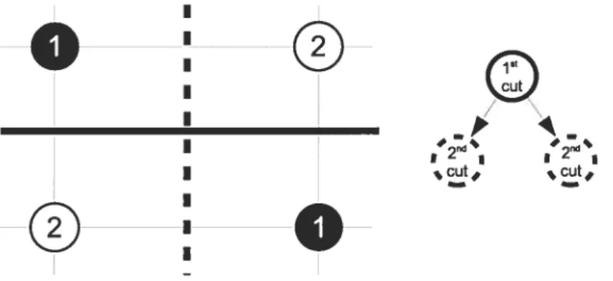
AB.SINGLE and AB.MuLTI. Figure 2.4 shows a simple example of tire differences among tire two approaches. Tire multi-class version of tire tree algorithm clescribed in Section 2.3.2 can use either tire single or tire multi-threshold approach, as each node of tire tree behave like a simple clecision stunrps. h this work we will refer to AB.TREE as the single-threshold version.
4 1
21
31111 1 22 11 2
122211
322322 3 33 33 3
-i1
3
211111 2 2 11 2 i2 221
I
32232213 33 33 3
Figure 2.4: Tire two different ways of treating tire nruiticlass probieur with stunrps. In tire first one on tire top (AB.SINGLE) there is just a single threshoid, which is selected by nrininrizing tire overali weighted error. In tire bottour one (AB.IVIULTI),
each ciass finds its owu threshold, computed by conrparing tire ciass against ail of tireur. Tire arrows represent tire eienrents of the y vector.
Tire aligument vector y ca be optimized eleureirt-wise in the foliowing way. For a given binary classifier4 , and for ail classes £ 1
K,
we define= wf{(xj)yj, — (t) = wf {(xj)yj,e = +1}, (2.28) i=1 [teo
34 With this notation, for a given vote vector y = (y1, . .. ,vj), it is clear that
Z
(_{ve =+11
+e+{ve = _i}),6 (t+ll{v +1} + {v _i}),
E0 =
If abstention is not used, the values of the alignment vector are simply
f
1 if+ut = (2.29)
otherwise.
Both strategies AB.SINGLE and AB.MuLTI share the same complexity, which
is O(kdn). This assuming that the feature vector projections (x,... ,x) are
ordered beforehand. If this is not true, the sorting tue brings the complexity to O(kdn 10g n). The cost of the whole algorithm is respectively O (nd(kT + log n))
auJ O (n logndkT) tues.
Once the weak classifier is selected, the coefficient cr is computed in the sanie way as (2.2). In the final step of each iteration, we re-weight the data points using the forrriula (t) t (t) (t) (t+1) — exp ç—ci yh (xi) wie — Z(t)
where Z(t) is the usual iorma1ization factor such that = 1.
After T iterations, the algorithin outputs a vector—valueci discriminant function
g(x) = Za(t)h(t)(x)
35 that is,
f(x) = argmax ge(x).
Algorithrn 3 AdaBoost.IVIH Input: D, WEAK(D,w(t)), T 1: for j — 1 to n do 2: for—1tokdo (1)
J
5 if ye = 1, 3: t {Imtiahze weights} I 2n(k—1) otherwise. 4: end for 5: end for 6: for t — 1 to T do 7: — WEAK(D.w(t)) (t) (6 8: E : Zh(x)y,,We 9: in (i) 10: for j — 1 to n do 11: forf—1tokdo (t+1) ‘)exp(_c(t)y (xi)) 12: zt) 13: end for 14: end for 15: end for16: return JT() = argmax
e
By sorting f(x) we can obtain a simple rank of the classes, which can be useful in the situations where an example has not well defined class (borderline) or it belongs to many classes, as it is often the case with music. The described method is summarized in Algorithm 3.
The extension of ADABOOST.MH to regularization cloes not require any par ticular modification of the algorithm as only () and the early stopping criterion have to be changeci.
In this work we collsidered also abstention. We do not leave the decision to the weak learner as usual, but we add O to the decisions of the vote vector y. This is done by optimizing (2.26) with a greedy algorithm (that. for the time being, is
{Find optimal weak classifier}
{
Compute the weighted error}{
Compute the confidence}T
{Re-weight the points}
36 not proved to be optimal in terms of (2.27)). We first set y as iII (2.29). Then, in an iteration over the labels, we select the “best” element ofy to set to O, that is, the one that decreases (2.27) the most. The algorithm stops when (2.27) does not decrease anymore.
2.5.3 AdaBoost.MO
In the same article in which they suggested the previous algorithm, Schapire and Singer proposed also another variation called AdaBoost.MO, in which the multiclass problem is, again, partitioned into a set of binary problems. This ap proach was first proposed by Dietterich and Bakiri in 1995 [D395] in a somewhat different setting. They suggest using error correctillg output codes (ECOC), which they consider to be desiglled to separate classes far from each other in terms of their symmetric difference, to map the label on binary sets.
Intuitively we can say that ifwe have a set where
Y
{appte, orange, CheTrg,carrot, potato} we cnn separate the points by mapping them into the binary repre seiltation
Y’
= {frv,it, uegetabÏe}. The more the sets are separatecl from each other(apples are ctoser to oranges than potatoes), the better the classification is likely
to be.
IViore formally let H : X —
Y
andY
{yi, ...,y} 5e our k-polychotomy.The decomposition of the k-polichotomy generates a set of L mapping functions
ÀL, where each subdivide the input pattern in two complementary sets (or
superclasses) Y3t and
Y7.
These sets contain each one or more classes of the original k-polychotomy, as showed in Figure 2.5, thus the mapping5 is defined as+1 ifytCY,
À(y) =
1 ifyCY;.
Note that À maps to subsets of an unspecified label set