Modal and non-modal linear stability of Poiseuille flow through a channel with a porous substrate

(1)

Science Arts & Métiers (SAM)

is an open access repository that collects the work of Arts et Métiers Institute of

Technology researchers and makes it freely available over the web where possible.

This is an author-deposited version published in:

https://sam.ensam.eu

Handle ID: .

http://hdl.handle.net/10985/18038

To cite this version :

Souvik GHOSH, Jean-Christophe LOISEAU, Wim-Paul BREUGEM, Luca BRANDT - Modal and

non-modal linear stability of Poiseuille flow through a channel with a porous substrate - European

Journal of Mechanics - B/Fluids - Vol. 75, p.29-43 - 2019

Any correspondence concerning this service should be sent to the repository

Administrator :

archiveouverte@ensam.eu

(2)

Modal and non-modal linear stability of Poiseuille flow through a

channel with a porous substrate

Souvik Ghosh

a,b,∗

, Jean-Christophe Loiseau

b,c

, Wim-Paul Breugem

a

, Luca Brandt

b

a_{Process and Energy Department, Delft University of Technology, 2628 CB Delft, The Netherlands}

b_{Linné FLOW Centre and SeRC (Swedish e-Science Research Centre), KTH Mechanics, SE-100 44 Stockholm, Sweden} c_{Laboratoire DynFluid, Arts et Métiers ParisTech, 75013 ParisFrance}

Keywords: Porous channel flow Instability

a b s t r a c t

We present modal and non-modal linear stability analyses of Poiseuille flow through a plane channel with a porous substrate modeled using the Volume Averaged Navier–Stokes (VANS) equations. Modal stability analysis shows the destabilization of the flow with increasing porosity of the layer. The instability mode originates from the homogeneous fluid region of the channel for all the values of porosity considered but the governing mechanism changes. Perturbation kinetic energy analysis reveals the importance of viscous dissipation at low porosity values while dissipation in the porous substrate becomes significant at higher porosity. Scaling analysis highlights the invariance of the critical wavenumber with changing porosity. On the other hand, the critical Reynolds number remains invariant at low porosity and scales as Rec ∼ (H/δ)1.4at high porosity whereδis the typical thickness of the vorticity layer at the fluid–

porous interface. This reveals the existence of a Tollmien–Schlichting-like viscous instability mechanism at low porosity values, and Rayleigh analysis shows the presence of an inviscid instability mechanism at high porosity. For the whole range of porosities considered, the non-modal analysis shows that the optimal mechanism responsible for transient energy amplification is the lift-up effect, giving rise to streaky structure as in single-phase plane Poiseuille flow. The present results strongly suggest that the transition to turbulence follows the same path as that of classical Poiseuille flow at low porosity values, while it is dictated by the modal instability for high porosity values.

1. Introduction

Flows over porous media are encountered across diverse nat-ural and industrial processes such as porous river beds, transpi-ration, water filttranspi-ration, catalytic bed reactors, ground oil wells, geological flows etc. Among the different specific applications we mention cross-flow filtration in tubular membranes [1], convec-tive/transpiration cooling in porous gas turbine blades [2], fluid flow over flexible and rigid plant canopies and monami [3,4], alteration of near-wall turbulence by wall suction [5] and biological flow through lungs and kidneys [6,7]. Clearly these applications cover a wide range of flow speeds and permeabilities, from laminar to turbulent flows.

1.1. Models for porous media

Literature studies suggest discrepancies in modeling porous media flows in terms of using appropriate transport equations.

∗

Correspondence to: Department of Mathematics, Imperial College London, London SW7 2AZ, United Kingdom.

E-mail address:s.ghosh17@imperial.ac.uk(S. Ghosh).

The starting empirical relation for modeling flow through porous media was provided by Darcy (1856) but with specific restrictions on the range of validity of the relation. This empirical relation was not in good agreement with the experimental results by Wright [8] and Dybbs and Edwards [9]. Giorgi [10] derived the modeling equa-tions for flows through rigid porous media using matching asymp-totic conditions (Oseen approximation) considering the non-linear Forchheimer term along with the Darcy term. Lage [11] provided a detailed description of the limitations of Darcy equation and the modified transport equations used for porous media flows. Since then, different approaches have been used to simplify the description of the porous region. Physics-based assumptions are considered for the flow inside the porous layer and at the interface to couple the flow between fluid and porous regions. One such approach was used by Wagner and Friedrich [12] who assumed no-slip conditions for azimuthal and axial velocity components with a wall permeability condition for the radial velocity component to study turbulent flow through circular permeable pipes. Another approach reduces the flow inside the porous region to an adequate boundary condition at the fluid–porous interface. This approach was considered by Hahn et al. [13] for direct numerical simulations of turbulent channel flow over porous walls: it amounts to zero

(3)

wall-normal velocity at the fluid–porous interface. Even though these earlier approaches provided some insight into the effects of wall permeability, they could not ascertain whether the assump-tions were reasonable enough. Another issue concerns the possible strategies to model the multiphase porous region, being e.g. a packed bed of cubes [14], spheres [15–17] or solid cylinders [18]. The first accurate transport equations for modeling the flow inside the porous region, called Volume-Averaged Navier–Stokes (VANS) equations were derived by Whitaker [19–21]. The VANS equations were derived using the concept of volume averaging based on the continuum approach, where the flow in the porous region is treated as a continuum and coupled to the flow in the fluid region. Different modeling approaches have been formulated for coupling the flow at the fluid–porous interface. Beavers and Joseph [22] and Ochoa-Tapia and Whitaker [23] proposed the use of jump conditions to match the flow in the homogeneous fluid and porous regions, circumventing the need to explicitly model the flow inside the interface region. Ochoa-Tapia and Whitaker [23] showed that the length constraints required for the validity of VANS equations in the interface region are not fulfilled. In a related study, Ochoa-Tapia and Whitaker [24] explicitly modeled the macroscopic flow in the interface region by proposing a variable-porosity model, which was used to compute the local variation in the permeability in the (Darcy-)Brinkman equation. This was successfully validated against experiments of Beavers and Joseph [22]. The direct nu-merical simulations of turbulent porous channel flows by Breugem and Boersma [14] also showed good agreement between the direct approach where the flow has been simulated explicitly around the pores (using an Immersed boundary method to enforce the no-slip and no-penetration boundary conditions on the cubes defining the porous phase) and the continuum approach (using the VANS equations with variable-porosity model at the interface region). The continuum approach is computationally more efficient than the direct approach but the former requires a closure model for the drag force and sub-filter scale stress, see Breugem et al. [16] for details. In this paper, we follow the same modeling approach as in Breugem et al. [16].

1.2. Stability of flow over a porous layer

The porous layer destabilizes the flow as reported by Beavers et al. [25] for the first time. The first experiments were performed by Sparrow et al. [26] to predict the stability of laminar chan-nel flow with a permeable wall. They also performed the two-dimensional linear stability analysis using Darcy’s law with the in-terface matching conditions proposed by Beavers and Joseph [22]. Their experimental and numerical results showed that the wall permeability destabilizes the flow at lower Reynolds numbers than for an impermeable wall. A detailed modal linear stability analysis for channel surrounded with two adjacent porous walls was presented by Tilton and Cortelezzi [27] using the VANS equa-tions [21] with matching stress conditions in terms of interface coefficient as given in Ochoa-Tapia and Whitaker [23,28]. Tilton and Cortelezzi [27] neglected inertial effects in the porous region for small values of permeability. These authors considered same permeability values for both porous walls with fixed porosity, height of porous layers, and interface coefficient. They concluded that small increments in the wall permeability can significantly decrease the stability of the channel flow as compared to classical Poiseuille flow. Chang et al. [29] studied the linear stability of Poiseuille flow over a porous layer by a two-domain approach with Navier–Stokes equations for the fluid region and Darcy equation for the porous layer, with the coupling interface conditions as in Beavers and Joseph [22] and Jones [30]. These authors found the results to be independent of the interface conditions used. Their work marked the existence of three competing modes hav-ing different characteristics but driven by the shear stress of the

Poiseuille flow in the fluid region. The modal stability analysis was further extended to specific cases of porous materials like foametal and aloxite by Tilton and Cortelezzi [31] who examined the char-acteristics of unstable modes for varying permeability, porosity, height of the porous layer and momentum transfer coefficient. The instability of classical Poiseuille flow in a fluid–porous system was studied by Liu et al. [32] using the Brinkman equation instead of Darcy’s law. The interface condition used was the continuity of tangential and normal components of velocity and stress tensor as shown by Desaive et al. [33]. The flow instability character-istics were different with the Brinkman equation since only two instability modes appear. These authors therefore concluded that the specific model chosen for the porous region, has to be verified experimentally. A similar study of the instability of Poiseuille flow in a channel with a porous substrate was performed by Hill and Straughan [34], where the porous substrate was modeled using Darcy’s law with an intermediate Brinkman porous transition layer adjoining the channel region. This work was further extended by Hill [35] by considering a three layer configuration but with variable effective viscosity between the upper fluid region and the lower homogeneous porous region. In both studies [34,35], it has been observed that two different competing instability modes exist. A more recent linear stability analysis has been performed by Li et al. [36] considering the same modeling approach as in Tilton and Cortelezzi [27,31]. These authors reported the flow instability for varying values of the porous filling ratio with a fixed value of permeability. The main conclusion was that the configuration of a porous layer surrounded by channels was more stable as compared to the configuration of a channel surrounded by two porous walls. Even though the modal stability of porous channel flows have been extensively studied, a better understanding of the destabiliza-tion mechanism is still needed. In this paper, we present a detailed analysis to identify the origin, physical mechanism and the nature of the instability responsible for the destabilization in porous chan-nel flows. We perform the linear stability analysis using a primitive variable approach and discretize the linearized VANS equations us-ing a fourth-order dispersion-relation preservus-ing finite-difference scheme. First, we present an eigenmode analysis and identify the origin of the instability modes. We perform the energy analysis to get a clearer physical interpretation of the instability growth mechanism. However most of the previous research do not say much about the evolution of the nature of the instability mode as we go from low to high porosity values. In this context, the study by Singh et al. [37] classified the two different competing instability modes in flow through submerged seagrass bed. From linear sta-bility analysis and experiments, these authors labeled one of them as a Kelvin–Helmholtz mode modified by vegetation drag and the other one as an instability mode unrelated to a Kelvin–Helmholtz mode originating from the interactions between the vegetated and unvegetated regions. We make an attempt to ascertain the characteristics of the instability mode by performing the scaling analysis following a similar approach as in Singh et al. [37]. We de-fine the vorticity thickness using the phenomenological estimate of the velocity gradient at the interface, Beavers and Joseph [22]. However, new theoretical approaches have been presented in the works of Minale [38,39] and Carotenuto et al. [40], where stress conditions are used at the interface taking into account the mo-mentum transfer from the fluid region to both the solid and fluid phases in the porous region. We also perform a Rayleigh anal-ysis at high porosity value to clearly characterize the instability mode. To conclude, we perform a non-modal analysis to identify the optimal mechanism possibly responsible for early transition following the approach reviewed in Schmid [41]. The non-modal transient growth analysis for a plane channel flow with a porous substrate was studied by Scarselli [42] and Quadrio et al. [43] using the modeling approach in Tilton and Cortelezzi [31]. They

(4)

found maximum transient growth with increasing permeability associated with significant flow across the fluid–porous interface. They also found that the variation of porosity and the momentum transfer coefficient had minimal effect on the transient energy am-plification as compared to the effect on the linearly unstable region. This paper is organized as follows. The problem statement with the governing equations are presented in Section2whereas the numerical methods with their validation are reported in Section3. The results and discussions for the modal analysis, energy analysis and non-modal analysis are reported in Section4. The main con-clusions are provided in Section5.

2. Problem statement

2.1. Governing equations

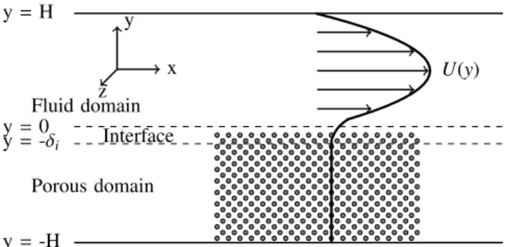
We analyze the instability in a plane channel flow with a porous substrate and denote the stream-wise, wall-normal and the span-wise directions as x, y and z, respectively. The flow domain can be divided into three different regions namely the homogeneous fluid region, the interface region and the homogeneous porous region. The homogeneous fluid region extends from y

=

0 to y

=

H and is delimited by an upper solid wall at y

=

H. The homogeneous porous region extends from y

= −

H to y

= −

δ

_i with a bottom solid wall at y

= −

H. The homogeneous fluid and porous regions are separated by an interface region extending from y

= −

δ

i

to y

=

0, seeFig. 1. The porous region is modeled as a packed bed of solid spheres with a specific value of the mean particle diameter, dp, and of the fluid volume fraction, defining the porosity

ϵ

[16]. In the porous region, the fluid flows only through the pores where it can still be modeled by the Navier–Stokes equations (at the microscopic scales). However at the macroscopic scales, the flow is modeled by the Volume-Averaged Navier–Stokes (VANS) equations. The derivation follows the work of Whitaker [21]. The dimensionless VANS equations (in intrinsic form) are thus given as [16],

∇

· [

ϵ

u

] =

0 (1)

∂

u

∂

t

= −

1

ϵ

∇

· [

ϵ

u

⊗

u

] − ∇

p

+

1 Reb

∇

2u

+

1

ϵ

Reb

∇

ϵ · ∇

u

−

1 Reb Fo Da

ϵ|

u

|

u

+

1 Reb

[ ∇

2

_ϵ

ϵ

−

ϵ

Da

]

u (2)

In the above, we denote by u both the fluid velocity in the fluid region and u

=

1

/

_V_f

∫

Vfu dV the volume-averaged fluid velocity

in the porous region, and by p the volume-averaged pressure. The averaging volume corresponds to a control volume with contribu-tion of solid and fluid phases i.e. V

=

Vf

+

Vs(Vfis the fluid volume

and Vsis the solid volume). The porosity

ϵ

is in general a function

of the spatial coordinates. The additional terms arising from the interactions with the solid matrix will be better introduced in conjunction with the derivation of the energy budgets.

For the configuration under investigation the porosity distribu-tion

ϵ

varies only along the wall-normal direction, from a constant value

ϵ

cin the porous region to 1 in the homogeneous fluid region.

The continuity of the porosity is ensured by the interface region with a porosity distribution function which varies rapidly over the thickness

δ

iof the interface layer as assumed in Breugem et al. [16].

Analytically, the porosity is given as,

ϵ =

⎧

⎪

⎨

⎪

⎩

1

,

0

≤

y

≤

H

−

6(

ϵ

c

−

1)(y

/δ

i)5

−

15(

ϵ

c

−

1)(y

/δ

i)4

−

10(

ϵ

c

−

1)(y

/δ

i)3

+

1

,

−

δ

i

≤

y

≤

0

ϵ

c

,

−

H

≤

y

≤ −

δ

i (3)

Fig. 1. Schematic diagram of the flow configuration and the coordinate system

adopted.

The VANS equations become invalid in the interface region but it has been shown in Breugem et al. [14] that a variable-porosity model at the interface is able to accurately couple the flow in the fluid region to that in the porous substrate.

The VANS equations(1)and(2)are non-dimensionalized with the thickness of the fluid region H and the bulk velocity Ubin the

fluid region. The bulk Reynolds number is defined as Reb

=

UbH

/

ν,

ν

being the kinematic viscosity of the fluid. The dimensionless parameters for the porous region are the Darcy number, Da

=

K

/

_H2 _{and Forchheimer number, Fo}

₌

_{F U}

˜

b. The permeability K

and Forchheimer coefficientF are defined as in Whitaker [

˜

21] and Breugem et al. [16]: K

=

d 2 p

ϵ

3 180(1

−

ϵ

)2

,

˜

F

=

ϵ

100(1

−

ϵ

) dp

ν

(4)

The value of permeability K varies with the local porosity in the porous region and reaches infinity in the homogeneous fluid region (

ϵ =

1).

The impenetrability of the solid spheres into the solid wall induces an unavoidable porosity variation in the real proximity of the bottom solid wall and the VANS equations are also not valid in this transition zone. However, the Brinkmann boundary layer along the solid wall at y

= −

H has a thickness proportional to

√

Kc,

which in our case is much smaller than the thickness H considered. Hence the solid wall at y

= −

H has negligible influence on the flow in the interface and fluid regions as long as the thickness H is sufficiently large, see Breugem et al. [16] for details. The mean particle diameter inside the porous layer is dp

=

0

.

01H and the

thickness of the interface region is chosen as

δ

i

=

0

.

02H [16]. Here

we did not vary

δ

ias it is reported in Ghosh [44] that its effect is

not particularly significant for the computation of critical stability parameters if this is chosen small enough as compared to

√

K (ϵc)

/

_ϵ_c_,

the length scale associated with drag.

2.2. Base flow

The stream-wise and span-wise invariant laminar base flow

U

=

(U(y)

,

0

,

0)T _{is solution to the following steady state VANS}

equations, 0

= −

∂

P

∂

x

+

1 Reb

∂

2_U

∂

y2

+

1

ϵ

Reb

∂ϵ

∂

y

∂

U

∂

y

−

1 Reb Fo Da

ϵ|

U

|

U

+

1 Reb

[

1

ϵ

∂

2

_ϵ

∂

y2

−

ϵ

Da

]

U (5)

It has been obtained numerically by solving the equation above by means of the Newton method implemented in the SciPy li-brary [45].

(5)

2.3. Linear stability equations

For the linear stability analysis, the flow variables are decom-posed into base flow and infinitesimal perturbations, Ui

=

Ui

+

ui

and p

=

P

+

p. The linear stability of the base flow U is dictated by the fate of the infinitesimal perturbation ui. Their dynamics are

governed by the linearized VANS equations,

∂

ui

∂

t

= −

1

ϵ

∂

xj (

ϵ

Uiuj

+

ϵ

uiUj)

−

∂

p

∂

xi

+

1 Reb

∂

2_u i

∂

x2 j

+

1

ϵ

Reb

(

∂ϵ

∂

xj

∂

ui

∂

xj

)

−

1 Reb Fo Da

ϵ[

U ui

+

Uiu

] +

1 Reb

[

1

ϵ

∂

2

_ϵ

∂

x2 j

−

ϵ

Da

]

ui (6)

These equations can be written in compact form as,

∂

t

[

I 0 0 0

] [

u p

]

=

[

A

−

G D 0

] [

u p

]

(7)

The expression of divergence D and gradient G operators and of A are given in Appendix. Because of a minor bug in the generalized eigenvalue solver in LAPACK,1the procedure described in Edwards et al. [46] has been used in order to project(7)onto a divergence-free vector space. The resulting system then reads,

∂

u

∂

t

=

Lu (8)

where L is the projection of the linearized Navier–Stokes operator. The solution to this initial value problem (IVP) is formally given by,

u(t)

=

exp(tL)u0 (9)

where u0is the initial condition.

2.4. Modal stability analysis

Being the linear dynamical system(8)autonomous in time t and homogeneous in the x and z directions, one can seek for solutions using the normal-mode ansatz. The perturbation u(x

,

y

,

z

,

t) is thus given by,

u(x

,

y

,

z

,

t)

= ˆ

u(y)e(iαx+iβz+λt) (10) Introducing this ansatz in Eq.(8)results in the following ordinary eigenvalue problem,

λˆ

u

=

Lu

ˆ

(11)

where

λ = σ +

i

ω

is the eigenvalue,

σ

being the growth rate of the instability,

ω

its circular frequency,

α

the real-valued stream-wise wavenumber, and

β

the real-valued span-wise wavenumber. 2.4.1. Energy analysis

The perturbation kinetic energy budget provides information on the nature of the instability growth mechanism. The energy budget is obtained by multiplying the complex conjugate of the perturbation velocity with the linearized VANS equations(6). Fur-ther taking the conjugate, applying the commutative property for the operations of conjugate derivative,

(

∂_∂f_x

)

∗

=

∂_∂f∗

x, and averaging,

the equation for the perturbation kinetic energy (PKE) E(y

,

t)

=

1 _{For more details, see}_{http://www.netlib.org/lapack/bug_list.html}_{. To the} au-thors knowledge, this bug has not been corrected.

(uiu∗i

/

2) in a porous medium becomes,

∂

E

∂

t

= −

{

1

ϵ

∂

xj

(

ϵ

uiu∗iUj 2

)

+

1 2

(

u∗_i

∂

p

∂

xi

+

ui

∂

p∗

∂

xi

)

−

1 Reb

∂

2

∂

x2 j

(

uiu∗i 2

)}

−

(

_u∗ iuj

+

uiu∗j 2

)

∂

Ui

∂

xj

−

1 Reb

(

∂

ui

∂

xj

)(

∂

u∗_i

∂

xj

)

+

1

ϵ

Reb

(

∂ϵ

∂

xj

)

∂

xj

(

uiu ∗ i 2

)

−

1 Reb Fo Da

ϵ(

Uuiu ∗ i

+

Uiuu ∗ i

) +

1 Reb

[

1

ϵ

∂

2

_ϵ

∂

x2 j

−

ϵ

Da

]

(

uiu ∗ i

)

(12)

The terms in curly bracket above correspond to the transport of energy and only redistribute the energy within the flow domain. These transport terms have no net contribution to the energy budget in the homogeneous fluid and porous regions (

ϵ

= constant) on account of the no-slip boundary condition at the walls and periodicity. The first term inside the curly bracket represents the transport due to perturbations (TRANS), the second term is the velocity–pressure-gradient term (VPG) and the third one is the viscous diffusion (VD) term.

Integrating Eq.(12)over the flow domain, the rate of change of the perturbation kinetic energy is written as,

∫

1 −1

∂

E

∂

tdy

= −

∫

1 −1

(

_u∗ iuj

+

uiu∗j 2

)

∂

Ui

∂

xj







WS dy

−

∫

1 −1 1 Reb

(

∂

ui

∂

xj

)(

∂

u∗_i

∂

xj

)







DIS dy

−

∫

1 −1 1 Reb Fo Da

ϵ(

Uuiu ∗ i

+

Uiuu ∗ i

)







FOR dy

−

∫

1 −1 1 Reb

ϵ

Da

(

uiu ∗ i

)







DAR dy

+

∫

1 −1 1

ϵ

Reb

(

∂

2

_ϵ

∂

x2_j

(

uiu ∗ i

) + ∂ϵ

_∂

_x j

∂

xj

(

uiu∗i 2

))







POR dy (13)

In the expression above, WS represents the production by the Reynolds shear stresses, DIS viscous dissipation, FOR and DAR the work of the Forchheimer and Darcy drag. These two terms are non-zero only in the porous region. The last term, denoted as POR, consists of two contributions: the first term corresponds to viscous porous drag and the second term refers to viscous transport due to local gradients of porosity.

Finally, using the normal mode expansion, it can easily be shown that the normalized rate of change of the perturbation kinetic energy Er, defined as,

Er

=

1 Ω

∫

Ω

∂

E

∂

tdΩ 1 Ω

∫

Ω EdΩ

=

1 2LxLz

∫

1 −1

∫

Lx 0

∫

Lz 0

∂

E

∂

t dz dx dy 1 2LxLz

∫

1 −1

∫

Lx 0

∫

Lz 0 E dz dx dy (14)

has to be equal to twice the growth rate

σ

of the eigenmode mode under scrutiny. HereΩrepresents the flow domain with Lx

=

2_απ

and Lz

=

2_βπ being the length of the domain in x and z directions

respectively.

2.5. Non-modal stability analysis

It is now well understood that linear modal stability only pro-vides information about the asymptotic behavior of disturbances,

(6)

while large transient amplifications at short time are still possi-ble and indeed responsipossi-ble for transition to turbulence in sim-ple shear flows [41,47,48]. The short-time energy growth can be several magnitudes higher than the initial perturbation energy as seen in the case of viscous channel flows [48–50]. From a math-ematical point of view, this large transient growth results from the non-normality of the linearized Navier–Stokes operator. In wall-bounded flows, the mechanism responsible for the maximum disturbance energy amplification is the lift-up effect, by which stream-wise vortices create strong streaks [see e.g. the review by Brandt [51]]. We perform here a transient growth analysis by considering the initial value problem given by Eq. (8) and the perturbation kinetic energy defined as,

E(u(t))

=

1 2

∫

Ω uHQ u dΩ

=

1 2

∫

Ω uH_FH_{F u d}_Ω (15)

where Q is the symmetric positive definite matrix, with Cholesky decomposition Q

=

FHF , assuring proper weighting of the

per-turbation velocity along the wall-normal direction. The optimal energy amplification G(t) is written as,

G(t)

=

max u0̸=0 E(u(t)) E(u0)

=

max u0̸=0

∥

u(t)

∥

2_E

∥

u0

∥

2E

=

max u0̸=0

∥

exp(tL)u0

∥

2E

∥

u0

∥

2E

= ∥

exp(tL)

∥

2_E

= ∥

F exp(tΛ)F−1

∥

2₂ (16)

whereΛis the diagonal eigenvalue matrix. Computing the norm of the matrix exponential, the largest possible transient growth, reduces to the computation of the largest singular value of the last term on the right-hand side of Eq.(16). The corresponding singular vectors provide the optimal perturbation and the associ-ated optimal response. See Schmid and Brandt [48] for more details about the relation between matrix norm and non-modal stability analysis.

3. Numerical methods and validation

The eigenvalue problem introduced in the previous section is discretized by means of a difference (FD) scheme. The finite-difference scheme is chosen as this method creates sparse matri-ces resulting in significant reduction in computational resourmatri-ces, when extending the present formulation to more complex flows, e.g. duct flows with only one homogeneous direction. The most-common FD schemes, however, give rise to dispersive errors at higher wavenumbers and it is thus necessary to optimize the coefficients over a range of wavenumbers in order to reduce these errors. One such way of optimization is using dispersion-relation preserving (DRP) schemes. DRP schemes are finite difference (FD) schemes for which the coefficients are evaluated in Fourier space over a designated scale of wavenumbers to reduce the numer-ical error [52]. Here, we will consider fourth-order spatial dis-cretization along the wall-normal direction resulting in a seven-point stencil. We follow the approach of Kim and Lee [53] and Bauer et al. [54] to derive the coefficients through the method of minimization of the error between the actual and the modified wavenumbers. We optimize the fourth order dispersion relation preserving (FODRP) schemes over a specific range of wavenumbers (k

≤

π/

2). As a consequence, only four points per wavelength are required to obtain a good resolution. In the specific case of plane channel flow with a porous substrate, we observe steep gradients of the base flow near the two walls of the channel and at the fluid–porous interface. Therefore, we incorporate a suitable grid

Table 1

Darcy number, Da for different values of porosityϵc.

ϵc 0.3 0.6 0.9 0.95

Da 3.06e−08 7.50e−07 4.05e−05 1.90e−04

stretching function over the FODRP discretized grid in order to increase the density of grid points in the vicinity of the walls and at the interface.

Convergence tests and error analysis for the eigenvalue prob-lem using FODRP schemes are presented in Ghosh [44]. The actual number of grid points used is N

=

193, which gives a convergence error of 0

.

01%. The implementation of the numerical code has been validated against the results of linear stability analysis of Poiseuille flow and Couette flow by Schmid and Brandt [48], see Ghosh [44].

4. Result and discussions

4.1. Base flow

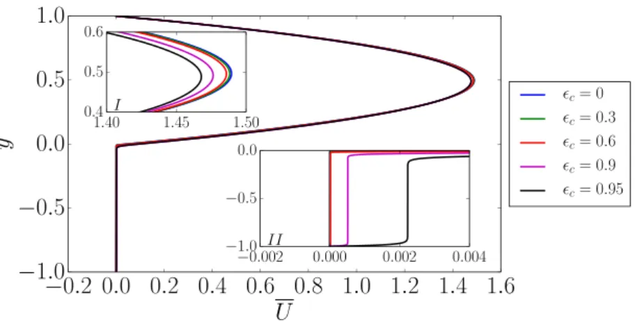
The base flow profile for the plane channel flow with a porous substrate is shown for

ϵ

c

=

0

,

0

.

3

,

0

.

6

,

0

.

9

,

0

.

95 in Fig. 2. For

ϵ

c

=

0, the flow is a regular Poiseuille flow in the upper fluid

region. When

ϵ

c

>

0, the flow displays an inflection point and

a distinct vorticity layer at the interface. In the limit

ϵ

c

→

1,

the classical Poiseuille parabolic flow is recovered over the entire height of the channel. The velocity magnitude within the porous region is negligible for

ϵ

c

=

0

.

3 and 0.6, while finite for

ϵ

c

=

0

.

9

and 0.95. As the bulk velocity is maintained constant over the fluid region, a small reduction of the maximum velocity in the fluid region of the channel is observed for

ϵ

c

=

0

.

9 and 0.95.

The VANS equations used for modeling the porous substrate as densely packed bed of spheres implies dependence between the porosity

ϵ

cand the permeability Kc. Hence the reader is referred to

note that for the further results presented, any change in porosity indicates change in permeability, seeTable 1for the dimensionless permeability given by Darcy number Da at different values of porosity

ϵ

c.

4.2. Modal stability analysis

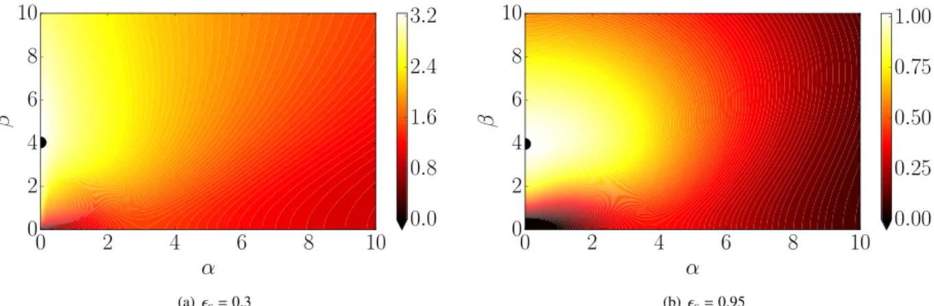
In the case of single-phase flows, the Squire theorem guarantees that the flow first becomes linearly unstable to two-dimensional waves. As the theorem cannot be extended directly to our problem, we start by checking that a similar conclusion applies also to the stability of a plane channel flow with a porous substrate described by the VANS equations. Lauga and Cossu [55] show that the Squire theorem can be extended to the case of slip channel flows, whereas Zhang et al. [56] demonstrate that two-dimensional modes are the first to become unstable in channel flow of polymer suspen-sions although the Squire theorem cannot be extended to this case directly. We therefore proceed by numerically investigating the first modes that become unstable. The least stable eigenval-ues in the

α − β

plane are shown inFig. 3for porosity values of

ϵ

c

=

0

.

3 and 0.95. In both cases (and others not reported

here), the least stable eigenvalues are confined along the

β =

0 axis and we thus assume that the flow first becomes linearly unstable to two-dimensional waves. Similar conclusions have been reached by Tilton and Cortelezzi [31] for a similar flow configura-tion. Hence for the neutral curve calculations presented here, only two-dimensional perturbations (i.e.

β =

0) are considered.

(7)

Fig. 2. Base flow velocity profile as a function of the porosityϵc. The insets I and II depict the close-up view of the velocity profile within the fluid and porous phase. The

parameters considered are Reb=2000 andδi=0.02 respectively.

Fig. 3. Contour plot of the growth rate of least stable mode in theα − βplane. The blue line represents the contour for growth rate=0. The parameters considered are (a) (Reb, ϵc)=(8000,0.3), (b) (Reb, ϵc)=(3000,0.95) andδi=0.02 for both cases. (For interpretation of the references to colour in this figure legend, the reader is referred to

the web version of this article.)

Fig. 4. Neutral stability curves for different values of the porosity,ϵc∈ [0,0.95]. In all cases, the thickness of the porous–fluid interface is set toδi=0.02.

Table 2

Comparison of growth rateσof the least stable eigenvalue for different values of porosityϵcandα =2 for all cases.

Reb ϵc=0 ϵc=0.3 ϵc=0.6 ϵc=0.9 ϵc=0.95

3000 −0.04798347 −0.04781321 −0.04598435 0.04679111 0.27738312 8000 0.00155281 0.00187691 0.00570383 0.18732385 0.46792848

4.2.1. Neutral curves

The neutral curve for different values of porosity in the range 0

≤

ϵ

_c

≤

0

.

95 are reported inFig. 4in the Re

−

α

plane. These

results are obtained with a constant thickness of the interface region (

δ

i

=

0

.

02).

For

ϵ

c

=

0 the critical Reynolds number based on the bulk

velocity and the channel width is Rec

=

7696

.

27,

correspond-ing to the classic value of 5772.2 uscorrespond-ing the centerline velocity and half-channel height. The critical Reynolds number does not change significantly as the porosity value is increased to

ϵ

c

=

0

.

3. Further increasing the porosity, however, results in a drastic reduction of the critical Reynolds number, in agreement with the results by Tilton and Cortelezzi [31] in a similar configuration and for increasing permeability. The critical stream-wise wavenum-ber

α

c increases from 2.04 for

ϵ

c

=

0 to 2.78 for

ϵ

c

=

0

.

95.

(8)

Fig. 5. (a) Eigenspectrum and wall-normal velocity component of (b) the wall eigenmode ( ), (c) the center eigenmode (•), and (d) the damped eigenmode ( ) for (Reb, α, ϵc)

=(8000, 2, 0.3). (For interpretation of the references to colour in this figure legend, the reader is referred to the web version of this article.)

Fig. 6. (a) Eigenspectrum and wall-normal velocity component of (b) the least stable wall eigenmode ( ), (c) the 1st porous eigenmode (▼), and (d) the 2nd porous eigenmode

(•) for (Reb, α, ϵc)=(8000, 2, 0.95). The inset in (a) shows the zoomed view of the 1st and 2nd porous modes. (For interpretation of the references to colour in this figure

(9)

changes significantly with the porosity of the medium, the critical stream-wise wavenumber

α

c is less sensitive to the variation of

porosity. As shown in the figure, however, the unstable region becomes larger as the porosity increases, spanning over a larger set of wavenumbers at fixed Reynolds number. This characteristic feature has been also reported by Tilton and Cortelezzi [31] for increasing permeability.

Finally, we consider the growth rate pertaining to the least stable mode for different values of porosity at Reb

=

3000 and

8000, seeTable 2. The growth rate of the least stable eigenvalue is essentially unchanged at

ϵ

c

=

0

.

3, corresponding to the case of

a fully packed bed of spheres, as also shown for lower values of permeability by Tilton and Cortelezzi [31]. As the value of porosity becomes higher, the growth rate increases drastically. The data in the table also suggest that the increase in the growth rate corre-sponding to an increase in Reynolds number is more significant for larger values of porosity.

4.2.2. Eigenspectrum and eigenmodes

Fig. 5(a) depicts the eigenspectrum for

ϵ

c

=

0

.

3 at Reb

=

8000

and

α =

2. For this low porosity case, the spectrum resembles that of single-phase Poiseuille flow, with the eigenvalues distributed over 3 different branches. We follow here the classic nomenclature. The eigenvalues on the uppermost left branch have their eigen-functions varying near the wall and the interface region and they are therefore labeled as wall eigenmodes, as shown by the shape of the wall-normal velocity component of the eigenmode inFig. 5(b). Like the case of plane Poiseuille flow with solid (impermeable) walls, the wall eigenmode is responsible for the instability for low values of porosity. The uppermost right branch of eigenvalues have their eigenfunctions varying near the center of the homogeneous fluid region as shown inFig. 5(c) and they are therefore labeled as center eigenmodes. The highly damped eigenvalues in the lower-most branch are labeled as damped eigenmodes. The corresponding wall-normal velocity component is shown inFig. 5(d): the per-turbations are confined within the homogeneous fluid region and disappear at the interface.

For high porosity value of

ϵ

c

=

0

.

95, the wall eigenmode has a

significantly larger growth rate, seeFig. 6(a). It is strongly affected by the porous region and the perturbation velocity is non-zero at the interface. This is due to weakening of the wall-blocking and wall-induced viscous effects near the permeable wall [57], which accounts for the transpiration velocity into the porous region. As depicted inFig. 6(b), the perturbation velocity now has a strong reversal at the interface. A similar feature has been reported by Chang et al. [29] and Hill and Straughan [34] for lower values of the ratio between the depth of the fluid and porous region. The transpiration velocity into the porous region becomes significant at high porosity values, while it decays inside the porous region. It is also interesting to observe the appearance of a new branch of eigenvalues in the eigenspectrum (indicated by ▼ and

•

in

Fig. 6a). This branch originates from the porous region and its

modes are therefore labeled as porous eigenmodes, see Tilton and Cortelezzi [31]. The wall-normal component of the eigenmode pertaining to the two least stable eigenvalues of the porous branch are depicted inFig. 6(c)–(d), to confirm that these highly stable modes only exist within the porous layer.

4.2.3. Energy analysis

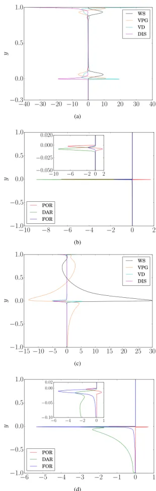
The perturbation kinetic energy budget of unstable normal modes has not been presented for the channel flow with a porous substrate earlier. The spatial distribution of the different terms in the perturbation kinetic energy budget in Eq.(13)is presented in

Fig. 7for low

ϵ

c

=

0

.

3 and high

ϵ

c

=

0

.

95 values of porosity. To

provide a good comparison over different ranges of porosity, all the terms in the perturbation kinetic energy budget are normalized with the total dissipation (D

=

DIS

+

POR

+

FOR

+

DAR).

Fig. 7. Kinetic energy budget of the most unstable mode for (a), (b):ϵc=0.3 and

(c), (d):ϵc=0.95. The parameters considered are (Reb, α): (8000, 2) for both cases.

The inset in (b) and (d) shows the zoomed view of the energy budget near the interface. (For interpretation of the references to colour in this figure legend, the reader is referred to the web version of this article.)

(10)

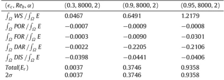
Table 3

Comparison of the total perturbation kinetic energy budget for different unstable modes with different values of (ϵc, Reb,α) with the growth rate of the least stable

eigenvalueσ. (ϵc, Reb,α) (0.3, 8000, 2) (0.9, 8000, 2) (0.95, 8000, 2) ∫ ΩWS/∫ΩE 0.0467 0.6491 1.2179 ∫ ΩPOR/∫ΩE −0.0007 −0.0009 −0.0008 ∫ ΩFOR/∫ΩE −0.0003 −0.0090 −0.0301 ∫ ΩDAR/∫ΩE −0.0022 −0.2205 −0.2106 ∫ ΩDIS/∫ΩE −0.0398 −0.0441 −0.0406 Total(Er) 0.0037 0.3746 0.9358 2σ 0.0037 0.3746 0.9358

Fig. 8. Normalized wall-normal integral of different contributions to the kinetic

energy budget for different values of porosity,ϵc ∈ [0.3,0.95]. The parameters

considered are (Reb, α): (8000, 2) for all cases. PD indicates dissipation in the porous

substrate and is equal to (POR+FOR+DAR). The data are normalized with respect to contributions atϵc=0.3.

For

ϵ

c

=

0

.

3, the shear production term (WS) is dominant

near the top wall and at the interface, which closely reminds of the energy distribution for the canonical Poiseuille channel flow. The viscous dissipation term (DIS) is strong near the top wall and interface, and is in balance with viscous diffusion term (VD), as also seen in the case of regular turbulent channel flow [see Mansour et al. [58]]. The WS term is locally balanced by the velocity–pressure gradient term (VPG) and to some extent by the VD term. The contributions due to porous drag (POR), Darcy drag (DAR) and Forchheimer drag (FOR) are seen in the porous region only. Here, the DAR term has the largest value, followed by the POR and FOR terms near the interface.

For high value of porosity,

ϵ

c

=

0

.

95 (lower panel inFig. 7), the

WS term increases significantly near the interface and is balanced by VPG and to a lower extent by DIS. This has also been reported by Breugem et al. [16] for the case of a turbulent flow in a channel with a porous substrate. Due to the apparent slip velocity at the interface, the viscous effects become less significant in this area. An interesting difference can be seen in the porous region near the interface, where the FOR term becomes larger than the DAR term. The VPG term increases significantly in the porous region in order to provide a local balance with the enhanced FOR and DAR terms.

The integrated contributions of each term of the perturbation kinetic energy budget, normalized with the contributions at

ϵ

c

=

0

.

3, are shown inFig. 8. Note that the total dissipation, sum of viscous dissipation and the dissipation in the porous substrate (PD

=

POR

+

FOR

+

DAR) is constant for different porosity values due to the normalization. The contribution due to the FOR term in-creases while the POR term contribution dein-creases as the porosity is increased from

ϵ

c

=

0

.

3 to

ϵ

c

=

0

.

95. The contribution due

to the DAR term also increases as the porosity is increased from

ϵ

c

=

0

.

3 to

ϵ

c

=

0

.

9 but drops as porosity is further increased

to

ϵ

c

=

0

.

95. However, the relative increase of the FOR term is

larger than that of the relative decrease in DAR term when porosity is increased from

ϵ

c

=

0

.

9 to

ϵ

c

=

0

.

95. At high porosity, the

critical Reynolds number decreases drastically and the instability in the flow can be explained by the substantial increase in the production term due to the Reynolds stress against the base flow shear. At high values of porosity, the integrated contribution of the FOR term is smaller than the DAR term. It has been shown in Breugem et al. [15] that a characteristic Reynolds number in the porous region defined as Rep

=

√

Kc

ϵcUs

/

νis the critical factor

in determining the contribution of the FOR term, where Usis the

apparent slip velocity at the fluid–porous interface. In the limit Rep

≪

1, the FOR term is very small as compared to the DAR term

for laminar flows, see Breugem [59] for details. Finally, it has to be noted that the normalized rate of change of the perturbation kinetic energy Er, obtained by summing the different

contribu-tions, is equal (to numerical errors) to 2

σ

as shown inTable 3, thus ensuring the correctness of the perturbation kinetic energy analysis.

4.3. Instability mechanism

A scaling analysis is presented in order to elucidate the physical origin of the instabilities. We have observed that the production related to mean shear increases with

ϵ

. However, the physical mechanism is different when varying the porosity. In order to support our assumption, a scaling is presented as in Singh et al. [37] for the monami in a submerged seagrass bed. For this scaling analysis, the critical parameter considered is the thickness of the vorticity layer

δ

at the fluid–porous interface, with the span-wise component of the base flow vorticity,

Ωz

=

∂

V

∂

x

−

∂

U

∂

y

= −

∂

U

∂

y (17)

According to the modified form of the Beavers and Joseph interface condition for a permeable wall [22],

dU dy

⏐

y=0

=

γ

(

Us

−

Ucp

√

Kc ϵc

)

(18)

where

γ

is a coefficient ofO(1) and Kcthe permeability for

ϵ = ϵ

c.

Usis the apparent slip velocity at the fluid–porous interface and

Ucpis the constant creep velocity in the porous region, which is

significant at high porosity values due to non-zero inertial velocity in the porous region.

Using (Us

−

Ucp) as the characteristic velocity difference, the

vorticity thickness

δ

can be written as,

δ = γ

(

Us

−

Ucp dU dy

⏐

y=0

)

,

(19)

Our analysis is performed with the fixed value ofdp

/

H

=

0

.

01. Com-paring Eqs.(18)and(19), the vorticity thickness can be expressed as,

δ ∼

√

Kc

ϵ

c

⇒

δ

H

∼

√

Da

ϵ

c

∼

ϵ

c 1

−

ϵ

c (20)

With increasing values of

ϵ

c, the vorticity thickness at the fluid–

porous interface increases significantly. Our analysis is performed separately for the low range of

ϵ

c, (0

.

3

≤

ϵ

c

≤

0

.

5) and the high

range of

ϵ

c, (0

.

9

≤

ϵ

c

≤

0

.

95) to clearly distinguish between

the two different physical mechanisms. We examine the scaling laws for the critical Reynolds number Recand the wavenumber

α

c

for the least stable mode in the low and high porosity ranges. The scaling power of the critical parameters as function of the vorticity thickness are shown inFig. 9.

(11)

4.3.1. Low porosity range

For low values of

ϵ

c, the critical Reynolds number Rec and

stream-wise wavenumber

α

cof the least stable mode are

indepen-dent of the vorticity thickness, Rec

∼

(H

/δ

)0 and

α

c

∼

(H

/δ

)0.

Both critical parameters are of order O(1). At low values of

ϵ

c,

the porous region almost behaves as a solid wall and hence the flow problem reduces to the classic regular Poiseuille channel flow. The underlying instability mechanism stems from the viscous mechanism of Poiseuille flow in the fluid region of the channel. The unstable mode characteristics are similar to that of a viscous instability mode and hence it is labeled as a Tollmien–Schlichting (TS) wave instability.

4.3.2. High porosity range

For high values of

ϵ

c= 0.9–0.95, the critical Reynolds number

Recand stream-wise wavenumber

α

cof the least stable mode can

be fitted by power laws, Rec

∼

(H

/δ

)1.4and

α

c

∼

(H

/δ

)−0.2. The

wavenumber

α

cdoes not change significantly over the range

ex-plored while Recchanges drastically when increasing the porosity.

It has been shown in Breugem et al. [16] that the permeability Reynolds number defined as ReK

=

√

Kc

ϵcuτ

/

ν is the discerning

parameter for the effect of the porous wall on the turbulent flow. To see if the same holds for laminar flow, we include the red line, corresponding to a value of the ratio

√

Kc

ϵcuτ

/

ν

=

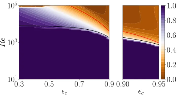
1 on top of the

contour of viscous dissipation to total dissipation (sum of viscous dissipation and dissipation in the porous substrate) for different porosity values inFig. 10.

The red line corresponds to the constant permeability Reynolds number ReK

=

1 and is obtained by calculating

√

Kc

/

_ϵ_c _{and u}_τ

from the bulk velocity Ubfor different values of porosity. The line

ReK

=

1 demarcates the transition from viscous dissipation to

dissipation by drag within the porous substrate. The red line scales as (H

/δ

)2 _{as compared to the scaling of the neutral line, Re}

c

∼

(H

/δ

)1.4. The scaling law Rec

∼

(H

/δ

)2represents the case where

the shear energy production from the fluid region is transported and dissipated completely in the porous region. The scaling Rec

∼

(H

/δ

)1.4_{suggests that the shear production from the fluid region}

is not entirely dissipated in the porous region and the contribution from the viscous dissipation in the fluid region is not negligible.

The unstable mode at high porosity values originates as a con-sequence of the interaction between the fluid and porous regions. The influence of the porous region on the fluid region near the interface becomes more pronounced as the porosity increases. A similar mode has been identified as a mode different from the Kelvin–Helmholtz (KH) mode by Singh et al. [37] for the flow through a submerged seagrass bed.

To conclude, we perform a Rayleigh analysis, i.e. we neglect the viscous terms in the stability problem for a set of stream-wise wavenumbers

α

chosen in the unstable regime, using the base flow computed for Reb

=

20000,

ϵ

c

=

0

.

95, seeFig. 11. We also solve the

viscous linearized VANS equations for different Rebin the unstable

regime, with the base flow obtained by solving equation(5)at the corresponding value of Reb. As shown in the figure, the unstable

eigenvalues converge to the Rayleigh solution with increasing Reb.

This confirms that the unstable mode at high

ϵ

c

=

0

.

95 follows

an inviscid instability mechanism in the presence of an inflection point.

4.4. Non-modal analysis

In this section, we investigate the effect of the porosity of the substrate on the non-modal growth of the disturbance energy. We start by displaying the maximum transient growth for the low-porosity case with

ϵ

c

=

0

.

3 at Reb

=

4000 and a high-porosity case,

ϵ

c

=

0

.

95 at Reb

=

300, in the

α − β

plane inFig. 12. The Reynolds

Fig. 9. Scaling of the critical parameters (Rec, αc) for the normal instability mode

as function of normalized vorticity thicknessδ/H at (a), (b): low [0.3–0.5] and (c), (d): high [0.9–0.95] porosity ranges.

numbers are chosen in the sub-critical range and well below the critical Reynolds number, Rec, for the onset of linear instability.

(12)

Fig. 10. Contour plot of ratio of viscous dissipation to total dissipation (viscous

dis-sipation+dissipation in the porous substrate) for two dimensional perturbations (β =0) at different values of porosity and Re. The black line (Re=Rec) denotes

the neutral curve and the red line represents√Kc

ϵcuτ/ν=1. (For interpretation of the references to colour in this figure legend, the reader is referred to the web version of this article.)

Fig. 11. Growth ratesσof the least stable mode in the rangeα ∈ [2.4,3.2]for ϵc = 0.95. The solution of the inviscid Rayleigh equation is compared with the

solutions of the viscous linearized VANS equations for different Rebwith the base

flow obtained by solving the actual steady state VANS equations.

Table 4

Maximum transient growth Gmaxat different stream-wise wavenumbersαin range

ϵc∈ [0,0.8]. The parameters considered are Reb=4000 andβ = βoptfor all cases.

The normalized maximum transient growth˜Gmaxis plotted inFig. 14.

ϵc=0 ϵc=0.3 ϵc=0.5 ϵc=0.7 ϵc=0.8 α =0, β =4 1761.98 1764.78 1764.97 1765.61 1766.67 α =1, β =5 656.70 653.39 653.24 654.60 659.37 α =2, β =5 336.52 333.92 333.83 334.90 338.72 α =3, β =6 202.08 199.93 199.81 200.18 201.93 α =4, β =8 134.04 132.59 132.48 132.57 133.45

The transient growth map reveals that the kinetic energy of the perturbation may grow by a factor of roughly 1500 before the perturbation eventually decays when

ϵ

c

=

0

.

3 and Reb

=

4000,

and by a factor 10 for

ϵ

c

=

0

.

95 and Reb

=

300. The maximum

transient growth in the

α

and

β

wavenumber space is shown as a black dot in the map.

At both low and high values of porosity, the maximum energy amplification takes place for stream-wise invariant perturbations (

α =

0). This characteristic feature has also been observed in the stability analysis by Scarselli [42] and Quadrio et al. [43], for the flow between two porous walls. We have considered the maximum energy growth for perturbations with

α =

0 and different values of the porosity between 0 and 0.95 at sub-critical Reband observed

that the maximum transient growth takes place for

β ≈

4 in all cases. As the thickness of the homogeneous region is H and not 2H as usually assumed for channel flow with rigid walls, the optimal perturbations have therefore the same spatial scales in the two cases.

Table 5

Maximum transient growth Gmaxat different stream-wise wavenumbersαin range

ϵc ∈ [0.8,0.95]. The parameters considered are Reb =300 andβ = βoptfor all

cases. The normalized maximum transient growth˜Gmaxis plotted inFig. 15.

ϵc=0 ϵc=0.8 ϵc=0.85 ϵc=0.9 ϵc=0.95 α =0, β =4 10.22 10.25 10.26 10.29 10.42 α =1, β =4 9.20 9.25 9.27 9.32 9.62 α =2, β =5 7.73 7.70 7.71 7.75 8.02 α =3, β =5 6.16 6.11 6.12 6.15 6.52 α =4, β =5 4.71 4.67 4.67 4.70 4.90

The optimal initial condition and the response are shown in

Fig. 13for low (

ϵ

c

=

0

.

3) and high porosity (

ϵ

c

=

0

.

95). The

figure reveals that the lift-up mechanism is responsible for the disturbance energy amplification also for the case of plane channel flow with a porous substrate and it is therefore a very robust mechanism in shear flows, as shown also in the presence of a dispersed phase [51]. The optimal initial condition consists of a span-wise periodic array of stream-wise counter-rotating vortices, while the optimal response consists of alternating high- and low-speed stream-wise velocity perturbations, usually referred to as the stream-wise streaks. For high porosity, there is a transpiration velocity into the porous medium due to the weakening of the wall-blocking effect resulting in a flux exchange at the interface.

Limiting ourselves to subcritical conditions, the transient dis-turbance growth is weak for high values of porosity due to the lower Reb. We therefore consider separately lower and higher

values of porosity. We first consider porosity values in the range

ϵ

c

∈ [

0

,

0

.

8

]

and report the maximum transient growth for varying

stream-wise wavenumber

α

at the optimal span-wise wavenum-ber

β

opt in each case. The normalized maximum energy

amplifi-cation

˜

Gmaxis obtained by normalizing Gmax(

ϵ

c

, α

) with respect to

Gmax(

ϵ

c

=

0

, α

) and is displayed inFig. 14. The absolute magnitude

of the largest transient growth is reported inTable 4. The data reveal that there is a small increment in the transient growth when increasing from

α =

0 to

α =

0

.

1, with subsequent small re-duction further increasing the stream-wise wavenumber for each

ϵ

c. For

ϵ

c

≤

0

.

5, the difference in transient growth is within 1%.

Scarselli [42] also reported minimal transient energy amplification with the variation of porosity for a similar flow configuration.

Considering also the data of the modal analysis discussed above leads to the conclusion that the transition to turbulence is most likely to follow the same path observed in classic Poiseuille flow in this range of porosity (

ϵ

c

<

0

.

6). In the porosity range (0

.

6

≤

ϵ

c

≤

0

.

8), the relative optimal energy amplification increases

with increasing porosity for finite

α

, seeTable 4. In this case, the maximum increase of the transient growth is around 1% (

α =

0

.

1

, β =

4). This is seen as an effect of the destabilization observed at larger

ϵ

c.

Next we consider the maximum transient growth at high poros-ity values (

ϵ

c

∈ [

0

.

8

,

0

.

95

]

), in the parameter space where the

flow is characterized by a strong modal stability driven by the inflection point of the mean profile at the interface. As above, we vary the stream-wise wavenumber

α

at the optimal span-wise wavenumber

β

opt. The normalized maximum energy amplification

˜

Gmax is again obtained by normalizing Gmax(

ϵ

c

, α

) with respect to

Gmax(

ϵ

c

=

0

, α

), seeTable 5andFig. 15. The plot shows that the

rel-ative optimal energy amplification increases when increasing the stream-wise wavenumber for each porosity under investigation. Here the maximum increase of the perturbation energy is of the order of 10% (

α =

3

, β =

5).

We summarize the stability of the flow under investigation

in Fig. 16. The black region depicts the region of modal

stabil-ity, with the mechanism explained in the previous section. The white line represents the neutral curve and the region below the white line represents the sub-critical regime. The color map

(13)

Fig. 12. Maximum transient energy growth (logarithmic scale) in theα − βplane for different values of porosity. The parameters considered are (a) (Reb, ϵc)=(4000,0.3)

and (b) (Reb, ϵc)=(300,0.95). (For interpretation of the references to colour in this figure legend, the reader is referred to the web version of this article.)

Fig. 13. Left: Velocity vectors in the cross-stream plane of the optimal initial condition and Right: Stream-wise velocity contours of the optimal response for different values

of porosity. The parameters considered are (a) (Reb, ϵc)=(4000,0.3) and (b) (Reb, ϵc)=(300,0.95) withα =0,β =4 for both cases.

displays the largest possible transient growth, optimized over the

α

and

β

wavenumber space. This is almost independent of the porosity

ϵ

c and it is attained by stream-wise independent

modes due to the lift-up effect, seeFig. 13and discussion above. Finally, the red dashed-line represents the numerical abscissa i.e.

the Reynolds number Re below which any perturbation mono-tonically decreases. We see that at high porosity values, the un-stable plane protrudes into the sub-critical regime substantially limiting the possibility for the transient energy amplification to occur. Hence, the transition to turbulence at high porosity values is

(14)

Fig. 14. Normalized maximum transient growth˜Gmaxin rangeϵc∈ [0,0.8]for different values of stream-wise wavenumberα. The parameters considered are Reb=4000

andβ = βoptfor all cases. The data are normalized with respect to Gmax(ϵc=0.3, α).

Fig. 15. Normalized maximum transient growth˜Gmaxin rangeϵc∈ [0.8,0.95]for different values of stream-wise wavenumberα. The parameters considered are Reb=300

andβ = βoptfor all cases. Right panel shows the zoomed view of˜Gmax. The data are normalized with respect to Gmax(ϵc=0.3, α).

Fig. 16. Contour plot of maximum transient energy growth (in log scale) optimized

overα-βwavenumber space for different porosity values at sub-critical regime (Re ≤ Rec). The black unstable region is separated by the solid white neutral

line (Re = Rec) and the red dashed-line denotes the numerical abscissa. (For

interpretation of the references to colour in this figure legend, the reader is referred to the web version of this article.)

expected to be dominated by the exponential growth of unstable modes.

5. Conclusions

The present work reports a detailed analysis of the modal and non-modal linear instabilities experienced by the flow through a plane channel with a porous substrate, in the limit of coupled porosity–permeability. Models exist for different porosity and per-meability, e.g. Rosti et al. [60] where it is shown that permeability, even at very low values has a greater effect than porosity. In Sec-tion5.1, we give a brief summary of the key results presented while concluding remarks and perspectives are given in Section5.2.

5.1. Summary

5.1.1. Modal stability analysis

The destabilizing effect of the porous substrate on the adjoining channel flow as seen from earlier studies [26,29,31,32,34–36] has been observed also here using the VANS equations to model the flow inside the porous substrate. The critical Reynolds number reduces drastically while the critical wavenumber of the instability mode is relatively constant when increasing the porosity. At low porosity, the unstable eigenmode shows similar features as that of the classical Poiseuille channel flow, as reported earlier by Tilton and Cortelezzi [31]. At higher porosity, the velocity of the unstable eigenmode confirms flow reversal at the fluid–porous interface as observed in Chang et al. [29], Hill and Straughan [34] and Tilton and Cortelezzi [31].

The perturbation kinetic energy budget shows similar contri-butions as that of a regular Poiseuille channel flow at low porosity values. Increased production of kinetic energy at the interface is observed with the increase in porosity due to the slip at the fluid– porous interface. This causes weakening of the wall-blocking and wall-induced viscous effects with a transpiration velocity into the porous layer as reported earlier by Breugem et al. [16] in turbulent flows. This phenomenon allows momentum exchange between the fluid and porous regions contributing to large Reynolds stresses making the flow more unstable. The energy analysis also reveals that at high porosity values, the dissipation in the porous substrate plays a major role yet the viscous dissipation in the fluid region is not negligible.

The scaling analysis reveals the instability originates from a Tollmien–Schlichting viscous mechanism at low porosity values. Rayleigh analysis shows the existence of an inviscid instability mechanism at high porosity values.