Weakly-Labeled Data and Identity-Normalization for Facial Image Analysis

WEAKLY-LABELED DATA AND IDENTITY-NORMALIZATION FOR FACIAL IMAGE ANALYSIS

DAVID RIM

D´EPARTEMENT DE G´ENIE INFORMATIQUE ET G´ENIE LOGICIEL ´

ECOLE POLYTECHNIQUE DE MONTR´EAL

TH`ESE PR´ESENT´EE EN VUE DE L’OBTENTION DU DIPL ˆOME DE PHILOSOPHIÆ DOCTOR

(G´ENIE INFORMATIQUE) SEPTEMBRE 2013

c

´

ECOLE POLYTECHNIQUE DE MONTR´EAL

Cette th`ese intitul´ee :

WEAKLY-LABELED DATA AND IDENTITY-NORMALIZATION FOR FACIAL IMAGE ANALYSIS

pr´esent´ee par : RIM David

en vue de l’obtention du diplˆome de : Philosophiæ Doctor a ´et´e dˆument accept´ee par le jury d’examen constitu´e de :

M. DESMARAIS Michel C., Ph.D, pr´esident

M. PAL Christopher J., Ph.D, membre et directeur de recherche M. BENGIO Yoshua, Ph.D., membre

ACKNOWLEDGEMENTS

I would like to express my deepest gratitude to my advisor Chris Pal, who has provided constant guidance and encouragement throughout my studies both at the Ecole Polytechnique de Montreal and also at the University of Rochester. I honestly do not know where I would be without his patience and efforts.

I would also like to thank Yoshua Bengio, Erik Learned-Miller, Gideon Mann and Michel Desmarais for their guidance and time as well.

I thank Ubisoft for both financial support and for providing the helmet camera video data used for our high quality animation control experiments. I also thank the Natural Sciences and Engineering Research Council of Canada (NSERC) for financial support.

Finally, I would like to express my gratitude to my family who have supported me more than I deserve and more than I can ever repay.

ABSTRACT

This thesis deals with improving facial recognition and facial expression analysis using weak sources of information. Labeled data is often scarce, but unlabeled data often contains information which is helpful to learning a model. This thesis describes two examples of using this insight.

The first is a novel method for face-recognition based on leveraging weak or noisily labeled data. Unlabeled data can be acquired in a way which provides additional features. These features, while not being available for the labeled data, may still be useful with some foresight. This thesis discusses combining a labeled facial recognition dataset with face images extracted from videos on YouTube and face images returned from using a search engine. The web search engine and the video search engine can be viewed as very weak alternative classifier which provide “weak labels.”

Using the results from these two different types of search queries as forms of weak labels, a robust method for classification can be developed. This method is based on graphical models, but also encorporates a probabilistic margin. More specifically, using a model inspired by the variational relevance vector machine (RVM), a probabilistic alternative to transductive sup-port vector machines (TSVM) is further developed. In contrast to previous formulations of RVMs, the choice of an Exponential hyperprior is introduced to produce an approximation to the L1 penalty. Experimental results where noisy labels are simulated and separate expe-riments where noisy labels from image and video search results using names as queries both indicate that weak label information can be successfully leveraged.

Since the model depends heavily on sparse kernel regression methods, these methods are reviewed and discussed in detail. Several different sparse priors algorithms are described in detail. Experiments are shown which illustrate the behavior of each of these sparse priors. Used in conjunction with logistic regression, each sparsity inducing prior is shown to have varying effects in terms of sparsity and model fit. Extending this to other machine learning methods is straight forward since it is grounded firmly in Bayesian probability. An experiment in structured prediction using Conditional Random Fields on a medical image task is shown to illustrate how sparse priors can easily be incorporated in other tasks, and can yield improved results.

Labeled data may also contain weak sources of information that may not necessarily be used to maximum effect. For example, facial image datasets for the tasks of performance driven facial animation, emotion recognition, and facial key-point or landmark prediction often contain alternative labels from the task at hand. In emotion recognition data, for

example, emotion labels are often scarce. This may be because these images are extracted from a video, in which only a small segment depicts the emotion label. As a result, many images of the subject in the same setting using the same camera are unused.

However, this data can be used to improve the ability of learning techniques to generalize to new and unseen individuals by explicitly modeling previously seen variations related to identity and expression. Once identity and expression variation are separated, simpler super-vised approaches can work quite well to generalize to unseen subjects. More specifically, in this thesis, probabilistic modeling of these sources of variation is used to “identity-normalize” various facial image representations. A variety of experiments are described in which per-formance on emotion recognition, markerless perper-formance-driven facial animation and facial key-point tracking is consistently improved. This includes an algorithm which shows how this kind of normalization can be used for facial key-point localization.

In many cases in facial images, sources of information may be available that can be used to improve tasks. This includes weak labels which are provided during data gathering, such as the search query used to acquire data, as well as identity information in the case of many experimental image databases. This thesis argues in main that this information should be used and describes methods for doing so using the tools of probability.

R´ESUM´E

Cette th`ese traite de l’am´elioration de la reconnaissance faciale et de l’analyse de l’ex-pression du visage en utilisant des sources d’informations faibles. Les donn´ees ´etiquet´ees sont souvent rares, mais les donn´ees non ´etiquet´ees contiennent souvent des informations utiles pour l’apprentissage d’un mod`ele. Cette th`ese d´ecrit deux exemples d’utilisation de cette id´ee.

Le premier est une nouvelle m´ethode pour la reconnaissance faciale bas´ee sur l’exploitation de donn´ees ´etiquet´ees faiblement ou bruyamment. Les donn´ees non ´etiquet´ees peuvent ˆetre acquises d’une mani`ere qui offre des caract´eristiques suppl´ementaires. Ces caract´eristiques, tout en n’´etant pas disponibles pour les donn´ees ´etiquet´ees, peuvent encore ˆetre utiles avec un peu de pr´evoyance. Cette th`ese traite de la combinaison d’un ensemble de donn´ees ´etiquet´ees pour la reconnaissance faciale avec des images des visages extraits de vid´eos sur YouTube et des images des visages obtenues `a partir d’un moteur de recherche. Le moteur de recherche web et le moteur de recherche vid´eo peuvent ˆetre consid´er´es comme de classificateurs tr`es faibles alternatifs qui fournissent des ´etiquettes faibles.

En utilisant les r´esultats de ces deux types de requˆetes de recherche comme des formes d’´etiquettes faibles diff´erents, une m´ethode robuste pour la classification peut ˆetre d´evelopp´ee. Cette m´ethode est bas´ee sur des mod`eles graphiques, mais aussi incorporant une marge probabiliste. Plus pr´ecis´ement, en utilisant un mod`ele inspir´e par la variational relevance vector machine (RVM ), une alternative probabiliste `a la support vector machine (SVM) est d´evelopp´ee.

Contrairement aux formulations pr´ec´edentes de la RVM, le choix d’une probabilit´e a priori exponentielle est introduit pour produire une approximation de la p´enalit´e L1. Les r´esultats exp´erimentaux o`u les ´etiquettes bruyantes sont simul´ees, et les deux exp´eriences distinctes o`u les ´etiquettes bruyantes de l’image et les r´esultats de recherche vid´eo en utilisant des noms comme les requˆetes indiquent que l’information faible dans les ´etiquettes peut ˆetre exploit´ee avec succ`es.

Puisque le mod`ele d´epend fortement des m´ethodes noyau de r´egression clairsem´ees, ces m´ethodes sont examin´ees et discut´ees en d´etail. Plusieurs algorithmes diff´erents utilisant les distributions a priori pour encourager les model´es clairsem´es sont d´ecrits en d´etail. Des exp´eriences sont montr´ees qui illustrent le comportement de chacune de ces distributions. Utilis´es en conjonction avec la r´egression logistique, les effets de chaque distribution sur l’ajustement du mod`ele et la complexit´e du mod`ele sont montr´es.

est ancr´ee dans la probabilit´e bay´esienne. Une exp´erience dans la pr´ediction structur´ee uti-lisant un conditional random field pour une tˆache d’imagerie m´edicale est montr´ee pour illustrer comment ces distributions a priori peuvent ˆetre incorpor´ees facilement `a d’autres tˆaches et peuvent donner de meilleurs r´esultats.

Les donn´ees ´etiquet´ees peuvent ´egalement contenir des sources faibles d’informations qui ne peuvent pas n´ecessairement ˆetre utilis´ees pour un effet maximum. Par exemple les en-sembles de donn´ees d’images des visages pour les tˆaches tels que, l’animation faciale contrˆol´ee par les performances des com´ediens, la reconnaissance des ´emotions, et la pr´ediction des points cl´es ou les rep`eres du visage contiennent souvent des ´etiquettes alternatives par rapport `a la tache d’internet principale. Dans les donn´ees de reconnaissance des ´emotions, par exemple, des ´etiquettes de l’´emotion sont souvent rares. C’est peut-ˆetre parce que ces images sont extraites d’une vid´eo, dans laquelle seul un petit segment repr´esente l’´etiquette de l’´emotion. En cons´equence, de nombreuses images de l’objet sont dans le mˆeme contexte en utilisant le mˆeme appareil photo ne sont pas utilis´es. Toutefois, ces donn´ees peuvent ˆetre utilis´ees pour am´eliorer la capacit´e des techniques d’apprentissage de g´en´eraliser pour des personnes nou-velles et pas encore vues en mod´elisant explicitement les variations vues pr´ec´edemment li´ees `a l’identit´e et `a l’expression. Une fois l’identit´e et de la variation de l’expression sont s´epa-r´ees, les approches supervis´ees simples peuvent mieux g´en´eraliser aux identit´es de nouveau. Plus pr´ecis´ement, dans cette th`ese, la mod´elisation probabiliste de ces sources de variation est utilis´ee pour identit´e normaliser et des diverses repr´esentations d’images faciales. Une vari´et´e d’exp´eriences sont d´ecrites dans laquelle la performance est constamment am´elior´ee, incluant la reconnaissance des ´emotions, les animations faciales contrˆol´ees par des visages des com´ediens sans marqueurs et le suivi des points cl´es sur des visages.

Dans de nombreux cas dans des images faciales, des sources d’information suppl´ementaire peuvent ˆetre disponibles qui peuvent ˆetre utilis´ees pour am´eliorer les tˆaches d’int´erˆet. Cela comprend des ´etiquettes faibles qui sont pr´evues pendant la collecte des donn´ees, telles que la requˆete de recherche utilis´ee pour acqu´erir des donn´ees, ainsi que des informations d’identit´e dans le cas de plusieurs bases de donn´ees d’images exp´erimentales. Cette th`ese soutient en principal que cette information doit ˆetre utilis´ee et d´ecrit les m´ethodes pour le faire en utilisant les outils de la probabilit´e.

TABLE OF CONTENTS DEDICATION . . . iii ACKNOWLEDGEMENTS . . . iv ABSTRACT . . . v R´ESUM´E . . . vii TABLE OF CONTENTS . . . ix

LIST OF TABLES . . . xii

LIST OF FIGURES . . . xiii

LIST OF APPENDICES . . . xiv

LIST OF ACRONYMS AND ABBREVIATIONS . . . xv

CHAPTER 1 INTRODUCTION . . . 1

1.1 Definitions and concepts . . . 2

1.1.1 Face Recognition . . . 2

1.1.2 Facial Expression Recognition . . . 2

1.1.3 Facial Key-point Localization . . . 2

1.1.4 Semi-Supervised Learning . . . 2

1.1.5 Weakly-Labeled Learning . . . 3

1.2 Contributions of the Research . . . 3

1.2.1 Research Questions . . . 3

1.2.2 General Objective . . . 4

1.2.3 Hypotheses . . . 4

1.2.4 Specific Contributions . . . 4

1.3 Organization of the Thesis . . . 5

CHAPTER 2 LITERATURE REVIEW . . . 6

2.1 Face Recognition . . . 6

2.1.1 Controlled Face Recognition . . . 6

2.2 Facial Expression Recognition . . . 14

2.2.1 Expression Parameterization . . . 15

2.2.2 Features for Expression Recognition . . . 16

2.2.3 Subject Independent Emotion Recognition . . . 17

2.3 Graphical Models in Machine Learning . . . 19

2.3.1 Graphical Models . . . 19

2.3.2 Logistic Regression . . . 22

2.3.3 Principal Component Analysis . . . 23

2.3.4 Conditional Random Fields . . . 25

2.3.5 Semi-Supervised Learning . . . 28

2.3.6 Weakly Labeled Learning . . . 31

CHAPTER 3 Sparse Kernel Methods . . . 34

3.1 Sparse Priors . . . 36

3.1.1 Laplacian . . . 37

3.1.2 Exponential . . . 41

3.1.3 Jeffreys . . . 44

3.1.4 Generalized Gaussian . . . 46

3.1.5 Sparse Bayesian Learning . . . 47

3.1.6 Variational Bayes . . . 48

3.2 Summary of Results . . . 54

3.3 Multi-class Variational Bayes with Exponential . . . 55

3.4 Structured Prediction with Sparse Kernel Priors : A Relevance Vector Random Field . . . 59

3.4.1 Learning, Inference and Approximations . . . 60

3.5 Experiments and Results . . . 62

3.6 Discussion . . . 64

CHAPTER 4 Face Recognition with Weakly Labeled Data . . . 65

4.1 Weakly Supervised Learning . . . 67

4.1.1 Null Category . . . 70

4.2 Experiments . . . 74

4.2.1 Google Images . . . 74

4.2.2 Baseline Experiments . . . 75

4.2.3 Weakly Labeled Google Images . . . 77

4.2.4 Artificial Data . . . 79

4.2.6 Labeled Faces in the Wild - Controlled Noise Experiments . . . 85

4.2.7 Youtube Video . . . 86

4.3 Discussion . . . 89

CHAPTER 5 Identity Normalization For Facial Expression Recognition . . . 90

5.1 Literature Review . . . 91

5.1.1 Performance-driven Facial animation . . . 91

5.1.2 Key-point Localization . . . 92

5.2 Model . . . 93

5.2.1 Learning . . . 94

5.3 Experiments . . . 96

5.3.1 Emotion Recognition . . . 97

5.3.2 Animation Control Experiments . . . 102

5.4 Identity-Expression Active Appearance Model . . . 104

5.4.1 Algorithm . . . 104 CHAPTER 6 CONCLUSION . . . 110 6.1 Limitations . . . 111 6.2 Future Work . . . 111 REFERENCES . . . 113 APPENDICES . . . 129

LIST OF TABLES

Table 3.1 Listing of sparse priors. For a discussion of Gaussian Mixtures and the

Garrote, see Appendix A. . . 37

Table 3.2 Best Results for MAP estimate with Laplace prior. NSV is the number of support vectors or non-zero weights. . . 40

Table 3.3 Exponential prior : Best Results . . . 44

Table 3.4 Jeffrey’s prior results . . . 45

Table 3.5 Best Resulting MAP estimate with Generalized Gaussian . . . 47

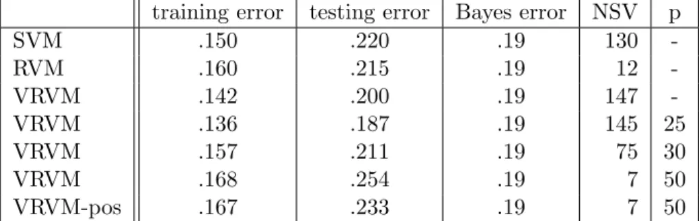
Table 3.6 Some tabulated results for Variational RVM, details are in text. . . 53

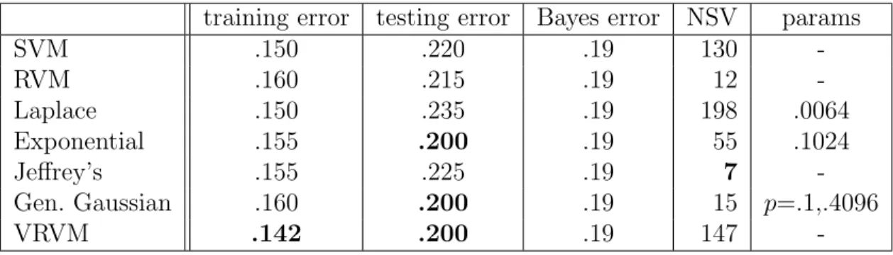
Table 3.7 Summary . . . 54

Table 3.8 This table summarizes the different accuracies for the adrenal segmentation problem using different models. ACA is the average class accuracy, PA is the pixel accuracy. . . 64

Table 4.1 Accuracy on the LFW combined with Google Image search tested on LFW . 79 Table 4.2 Results from artificial data set, showing error rates. . . 83

Table 4.3 Crossvalidation results on the LFW combined with Google Image search, crossvalidating for µ0. µ+ and µ− are estimated from the data, leaving µ0 as a free parameter. Again, the total probability is set to equal 1, effectively causing µ+ and µ− to scale but stay in proportion to each other. The results are show for Linear and Gaussian for a single held-out set. The figures in bold were used for the results shown in Table 4.2.3. . . 83

Table 4.4 Accuracy rates on Iris at different weak label accuracy rates. . . 85

Table 4.5 Accuracy using different proportions of labeled and unlabeled data using a known weak label accuracy parameter. The held out column presents the percentage of data used as unlabeled data. For our method, γ and µ0 were set to 1 and .50, respectively. To set µ+ and µ−are determined by the value of µ0 by setting µ+ = .75(1 − µ0), and µ− = .25(1 − µ0), the proportion of the remaining probability. Here we note that these values were found during crossvalidation, and that the classification rate during cross-validation using µ0 _{= 0, which would be the most similar to using the null-category noise} model was, on average, 14.75% lower. . . 86

Table 4.6 Accuracy on the YouTube faces. . . 88

Table 4.7 Accuracy on the LFW using the LFW augmented with Youtube faces as training data.. . . 88

Table 4.8 Accuracy on the YouTube faces using the LFW augmented with You-tube faces as training data. . . 89 Table 5.1 Summary of experiments described in this paper, numbers of the

sec-tion describing each experiment are given in parenthesis. . . 96 Table 5.2 Accuracy for JAFFE emotion recognition in percentage and Mean

Squared Error for bone position recovery experiments for JAFFE and Studio Motion Capture data, calculated per bone position, which lie in [−1, 1]. . . 98 Table 5.3 CK+ : AUC Results and estimated standard errors of the AU experiment . 100 Table 5.4 Comparison of confusion matrices of emotion detection for the combined

landmark (SPTS) and shape-normalised image (CAPP) features before and after identity normalisation. The average accuracy for all predicted emotions using the state of the art method in Lucey et al. (2010) is 83.27% (top table), using our method yields 95.21% (bottom table), a substantial improvement of 11.9%. . . 101 Table A.1 Best Results for MoG . . . 136 Table A.2 Results for Non-Negative Garrote . . . 140

LIST OF FIGURES

Figure 2.1 Example of “controlled” data, from Cambridge (1994). . . 8 Figure 2.2 Example of keypoints, from Wiskott et al. (1997) . . . 8 Figure 2.3 LFW dataset : Examples of the 250x250 images, varying illumination,

pose, occlusion. . . 9 Figure 2.4 Example of a sequence of FACS coded data from Cohn-Kanade dataset

(Kanade et al., 2000), which contains two views of the sequence. The AU of the final frame is coded as 1+2+5+27, Inner Brow Raiser+Outer Brow Raiser+Upper Lid Raiser+Mouth Stretch . . . 15 Figure 2.5 Example graphical models : 2.5(a) visualizes logistic regression, used

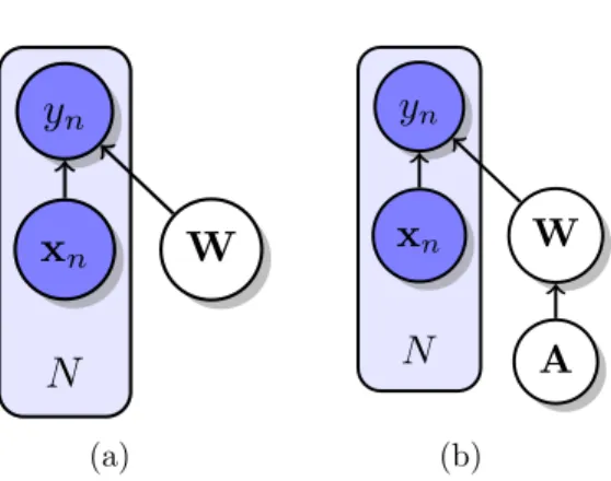
in Chapter 3 and Chapter 4. 2.5(b) visualizes Principal Components Analysis, discussed in Chapter 5. 2.5(c) visualizes a lattice structured CRF, developed further in Chapter 3. . . 20 Figure 3.1 Graphical model of supervised learning. x is the input, y is the label, W

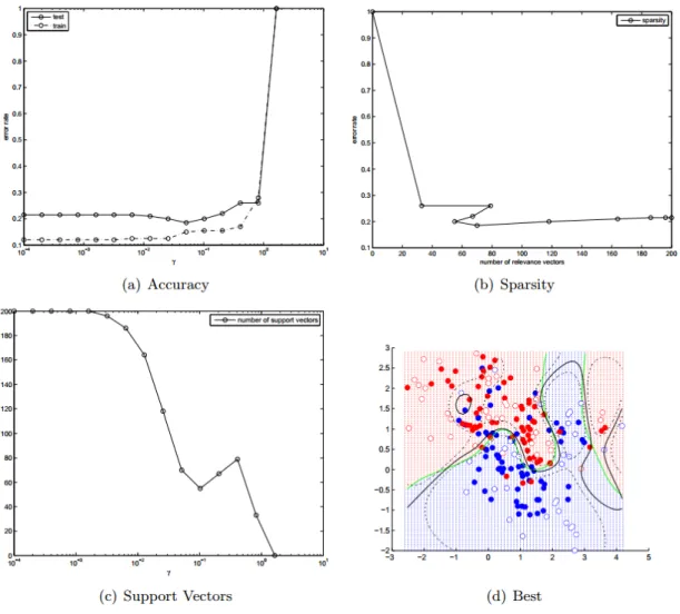
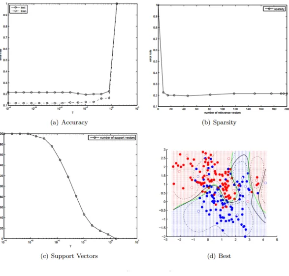
denotes model parameters. 3.1(a) depicts standard setting, in 3.1(b), A re-presents an additional hyper-parameter which is also equipped with a dis-tribution. . . 34 Figure 3.2 Visualization of some sparse prior distributions, details in text . . . 36 Figure 3.3 Laplace prior : accuracy, sparsity and number of support vectors (NSV). 40 Figure 3.4 Exponential prior : accuracy, sparsity and number of support vectors . 44 Figure 3.5 MAP classifier with Jeffrey’s prior . . . 45 Figure 3.6 Generalized Gaussian . . . 47 Figure 3.7 Variational RVM : Only positive relevance vectors are used. Details in

are in the text. . . 54 Figure 3.8 Segmentation examples using the model. Upper row shows results using

a contour model obtaining a pixel accuracy of 90.73 and 94.31 for two different slices and the lower row using the CRF obtains a pixel accu-racy of 96.72 and 97.48 respectively. The red is a modified shape prior and green is the segmentation result. . . 64

Figure 4.1 High performance recognition requires a large number of labeled examples in the uncontrolled case. Large amounts of weakly labeled data are easily obtainable through the use of image and video search tools. Many of these examples are either irrelevant or not the identity in question. We learn a classifier that does not require manual labeling of the weakly labeled data by accounting for the weak label noise. . . 66 Figure 4.2 Graphical model shown in Figure 3.1(b) augmented for semi-supervised

lear-ning. U is the index set of unlabeled examples, and L is the index set of the labeled examples. g denotes noisy label variables for examples with unob-served labels y. . . 67 Figure 4.3 Recognition accuracy for (top) the top 50 LFW identities, (bottom)

All LFW identities with four or more examples, or * 610 people and 6680 images. Tests performed in a leave 2-out configuration. ** The best threshold for adding new true examples was 0.5. *** The best threshold for adding new true examples was 0.8. . . 75 Figure 4.4 Estimate for weak-label accuracy based on search rank. . . 78 Figure 4.5 Effect of complexity and noisy label classification. The linear classifier

is not improved much using a semi-supervised method. However, with a more flexible classifier, the unlabeled data is much more useful. . . . 80 Figure 4.6 Data set, the green line denotes the bayes optimal classifier, training

points are large circles, details in text . . . 81 Figure 4.7 The use of noisy labels . . . 82 Figure 4.8 The pipeline output for one of Winona Ryder’s videos . . . 87 Figure 5.1 Graphical model of facial data generation. xij is generated from p(xij|vij, wi),

after sampling wi from an identity and vij from an expression-related distribution respectively. . . 93 Figure 5.2 The JAFFE dataset contains 213 labeled examples for 10 subjects.

Images for a single test subject, left out from training, shown here with predicted labels from our method. The data is shown in two sets of rows. The first row in each set is the original input data, the second a rendering of the mesh with corresponding bone positions predicted by the model. . . 97 Figure 5.3 Motion capture training data using a helmet IR camera. Example

pi-peline for a test video sequence. . . 103 Figure 5.4 Point-localization experiment evaluation, described in detail in text. . . 108 Figure A.1 MoG prior plot, K = 2, n = 20 . . . 135

Figure A.2 MoG prior plot, K = 2, n = 20 on full training set . . . 136 Figure A.3 Non-negative Garrote classifier . . . 140

LIST OF APPENDICES

LIST OF ACRONYMS AND ABBREVIATIONS

AU Action Unit

CHM Conditional Harmonic Mixing EBGM Elastic Bunch Graph Matching EM Expectation-Maximization FACS Facial Action Coding System FPLBP Four-Pass LBP

GEC Generalized Expectation Criteria GEM Generalized EM Criteria

GJD Gabor Jet Descriptor HMM Hidden Markov Model

ICA Independent Components Analysis ITML Information-Theoretic Metric Learning KLR Kernel Logistic Regression

LBP Local Binary Patterns

LDML Logistic Discriminant-based Metric Learning LFW Labeled Faces in the Wild

MAP Maximum A Priori ML Maximum Likelihood

ML-II Maximum Likelihood, Type 2 NMF Non-Negative Matrix Factorization OSS One-shot Similarity

PCA Principal Components Analysis

PPCA Probabilistic Principal Components Analysis RVM Relevance Vector Machine

SIFT Scale-Invariant Feature Transform SSL Semi-Supervised Learning

SVM Support Vector Machines TPLBP Three-Pass LBP

CHAPTER 1

INTRODUCTION

This thesis is about using machine learning for facial image tasks. Facial images are relatively easy to obtain, either as static images or sampled from video data. A wealth of useful information is stored in a facial image, for example, the identity and emotional state of the person depicted. For a number of reasons, it would be ideal to obtain such information automatically.

Artificial intelligence offers the possibility to do this using computation. One method of accomplishing this goal relies on obtaining a large data set of facial images and labeling them with the appropriate identity or emotional state. Then, the goal becomes to learn a function which maps the input image with the correct label.

However, obtaining labels for face images is time-consuming and expensive. However, for most computer vision tasks dealing with faces, very large amounts of labeled data are necessary to learn good functions.

Machine learning, and in particular, semi-supervised learning offers the possibility of avoiding much of the time-consuming and error-prone effort of labeling. However, in many instances, data are accompanied by additional information which may help for learning good functions.

In some cases, the additional information may be labels that are often incorrect. For example, these labels may come from an alternative classifier. In this case, the problem becomes how to incorporate these “noisy” or “weak” labels well.

In other cases, the data may have additional labels which are not a target. For example, for facial expression recognition, the data may come with identity labels. There is often additional or “side-information” which is not directly associated with the label, which may be useful for learning.

This thesis investigates the use of weak-supervision and leveraging side-information for facial image tasks, in particular face recognition and facial expression recognition.

This chapter introduces and defines these concepts, as well as outlines the objectives and main scientific hypotheses of the research. The final section presents the organization of the remainder of this proposal.

1.1 Definitions and concepts 1.1.1 Face Recognition

Face recognition is defined in this thesis as the action of determining the identity associa-ted with an image of a human face. In the context of computer vision, this is defined as the task of classifying a test image by identity. A related problem is face verification, in which the goal is to test whether two images belong to the same person. In essence, this can be viewed as in terms of binary image pair classification – same or not same. In this thesis, the face recognition problem is the identity classification task.

1.1.2 Facial Expression Recognition

Facial expression recognition is defined as the action of determining the label associa-ted with facial deformations usually associaassocia-ted with an emotive state, i.e.“anger,”“disgust,” “fear,” “happiness,” “sadness,” “surprise,” “contempt,” etc.This should not be confused with facial action unit detection, which is defined here as the identification of the non-rigid defor-mation of the face associated with facial muscle groupings. Expression labels, in this thesis, is synonymous with the emotion being expressed.

1.1.3 Facial Key-point Localization

A key step in many face recognition and facial expression recognition tasks is the need to detect and localize certain parts of the face – for example, eyes, nose and mouth. Face key-point localization is defined here as the action of determining the location of specific points in the face, such as the corners of the eyes, mouth and other face parts. Key-point locations are often used to build features for expression and facial action unit recognition. They can also be an important preprocessing step, as the key-points can be used to align facial images to remove certain kinds of variation. Variation which is the result of head or camera movement is also known as pose variation, as it depends on the pose of the person relative to the position of the camera.

1.1.4 Semi-Supervised Learning

The previous three subsections introduce the problem domains addressed in this thesis. Machine learning is the branch of artificial intelligence which attempts to produce systems built by learning from examples. In contrast to creating a complex system of hand-coded rules, machine learning attempts to create these systems automatically using examples.

If the learning algorithm is intended to create an algorithm which maps data to labels, and the algorithm is augmented with labels, this type of machine learning is known as supervised learning. This is because the algorithm is given a form of supervision in the form of labels. In contrast, without access to available labels, learning is called unsupervised learning.

Semi-Supervised Learning (SSL) is a type of machine learning which incorporates both unlabeled and labeled data. Typically, SSL is used in situations where labels are difficult to obtain but unlabeled data is plentiful, as in most computer vision tasks. For example, in object recognition tasks, images which may or may not contain the object are easy to obtain, but images which certainly contain the object are more difficult to obtain or to label in sufficient quantity.

There exist a range of algorithms which lie between the traditional labeled and unlabeled setting which could also be described as semi-supervised. This thesis will present a “weakly labeled” model, in which the unlabeled data is treated as labeled by a noisy process. Other side-information can also be used in lieu or in addition to labels. This thesis will also investi-gate the latter case, in which the information is used to obtain better input representations.

1.1.5 Weakly-Labeled Learning

Weakly labeled learning is defined in this thesis as a type of SSL in which the unlabeled data is accompanied by unreliable labels. The weak labels are not necessarily correct. In this case, supervised learning procedures can still be applied but are not necessarily appropriate. Many semi-supervised methods do not necessarily account for the presence of this kind of additional information.

1.2 Contributions of the Research

There are three main research questions posed in this thesis. Primarily they are concerned with how labeled and unlabeled data can be used to improve automatic face recognition and facial expression recognition.

1.2.1 Research Questions

– How can sparse kernel classifiers be designed in a way that allows them to be easily extended for other tasks ?

– How can weakly-labeled data improve face recognition ?

1.2.2 General Objective

The objective of the research proposed in this document is to investigate improving face recognition using weakly labeled data and improving facial expression recognition using iden-tity information. The main argument is that data often contain information that is not a feature or a label, which can and should be used effectively.

In facial recognition, this thesis seeks to show that incorporating weak labels, along with semi-supervised assumptions, can lead to better results than prior methods. For facial recog-nition, search queries to web repositories can be used as a source of unlabeled face image examples. The search engine then acts as a kind of classifier or labeler. However, the labeler is quite often incorrect. This thesis intends to show how proper handling of this informa-tion, combined with sparse kernel methods, can yield an improvement in face recognition performance.

Probabilistic sparse kernel methods are also an objective of this research. This thesis also intends to show how priors can be used to construct sparse kernel binary classifiers. Since they are probabilistic methods, they can be extended to other, more complex, models.

For facial expression recognition, instead of generating weakly labeled data, identity labels can be used as a kind of weak information. In this case, the assumption is that identity data can be used to construct representations for facial expression analysis in order to improve results. This research shows that this approach to additional information improves results for many expression tasks. In both cases, the methods discussed here obtain state-of-the-art results.

1.2.3 Hypotheses

Hypothesis 1 : Sparse kernel methods can be constructed in a way that allows them to be used as building blocks for other probabilistic methods.

Hypothesis 2 : The use of weakly labeled data can improve face recognition.

Hypothesis 3 : Identity information can and should be used to improve facial expression recognition.

1.2.4 Specific Contributions

This subsection presents the specific contributions that resulted from investigating these hypotheses.

– Novel probabilistic sparse kernel methods for binary classification and structured pre-diction.

– A method for learning classifiers using weakly-labeled data.

– Representations for expression recognition which normalize for identity.

– A method for improving facial expression recognition and performance driven animation using this representation.

– A method for improving key-point localization using identity normalization.

1.3 Organization of the Thesis

Chapter 2 provides a literature review of the topics addressed in this thesis, including a discussion of the state of the art in facial recognition and facial expression recognition. Also reviewed is work on graphical models, sparse priors, and semi-supervised learning, all of which are related to the methods used in the following chapters.

Chapter 3 is the first major theme of this thesis, which also provides many of the mathe-matical foundations required for the following chapters. In this chapter, sparsity and sparse priors are introduced and discussed in detail. Kernel methods are addressed as well. This chapter deals with the question of how to incorporate sparsity and kernel methods in a way which allows them to be extended to more complex models.

Chapter 4 is the second major theme of the thesis, applying the concepts from Chapter 2 to facial recognition with weak labels. Since unlabeled data is easily available, this chapter deals with the question of how to effectively use information associated with unlabeled data. That is, unlabeled data sometimes have natural “weak” labels that can be incorporated into learning. A novel method for weakly-labeled learning is fully developed.

Chapter 5 is the third and final major theme of the work, in which a probabilistic approach is used to “normalize” for identity. That is, representations for expression recognition often are subject to identity variation. This chapter introduces the idea of normalizing for identity by removing this variation. Since identity labels are often provided, this chapter deals with the question of how to effectively use identity information in order to improve facial expression recognition, performance-driven animation and facial key-point localization.

Chapter 6 concludes the thesis, summarizing the work presented in the thesis. The conclu-sion also suggests directions for further research.

CHAPTER 2

LITERATURE REVIEW

This chapter provides a review of many of the following chapters. First a review of face recognition literature is presented, with particular focus on face recognition in images obtai-ned from common sources such as the web and consumer photography. Then the literature of facial expression recognition, performance-driven animation and key-point localization are reviewed.

The machine learning methods used in the remaining chapters are reviewed as well in this chapter. In particular, the literature review focuses on kernel logistic regression and semi-supervised learning relevant to Chapter 3 and 4, as well as on factor analysis for chapter 5.

2.1 Face Recognition

Face recognition has a long history in artificial intelligence research. Many approaches and methods have been devised in order to help solve the problem. In earlier work, face recognition was focused on images in which variation was controlled to a large extent. That is, the facial images were collected in such a way to control for expression, pose, occlusion, background and other sources of variation. The field has moved toward more challenging data – images of faces captured in widely varying settings. The literature review is divided into two sections, first giving a brief overview of early work in Controlled Face Recognition and more recent work in Uncontrolled Face Recognition.

2.1.1 Controlled Face Recognition

Among the most widely cited facial recognition systems in the literature are those based on Principal Component Analysis (PCA) of intensity images, better known as eigen-faces, first presented by Sirovich et Kirby (1987) and used for recognition by Turk et Pentland (1991). In this method, test images are projected to a “face space” spanned by the eigen-vectors corresponding to the largest eigenvalues from the singular value decomposition of a training set. Turk et Pentland (1991) based classification on the Euclidean distance of an example projected into a the respective face spaces of particular classes. This general subspace method has since been extended using discriminant analysis (Fisher’s Linear Discriminant) by Belhumeur et al. (1996) and other types of factor analysis (e.g., ICA, NMF, Probabilistic

PCA) (Bartlett et al., 2002), (Guillamet et Vitria, 2002), (Moghaddam et Pentland, 1997)). Goel et al.. performed useful experiments with random projection which offer evidence that dimensionality reduction is a key task in facial recognition (Goel et of Computer Science University of Nevada, 2004).

Non-linear representations such as Locality Preserving Projection (LPP), a linear graph embedding method by Seung (2000) and later by Xu et al. (2010) and Sparsity Preserving Projections (SPP) ((Qiao et al., 2010)), used for locally linear manifold representations has widely been applied to face recognition. Moghaddam et al. (2000) showed that similarity me-trics, used commonly in Nearest Neighbor methods (NN), have also shown good performance. More recently, Wang et al.used a subspace created by merging KD-tree leaf partitions based on distance metrics and classification rates in order to improve facial recognition via LDA (Wang et al., 2011). However, most of these methods have been applied to controlled data-bases. Yang et Huang (1994) describes similar face detection issues with complex background variation. Zhang et Gao (2009) provides an excellent review of the problems that arise due to uncontrolled pose variation.

In earlier work, facial recognition was dominated by these subspace methods, which have generally reported excellent accuracy. However these systems, termed “holistic approaches” in Zhao et al. (2003), require either an infeasible number of training examples to determine a reasonable set of basis vectors in the presence of wide variation or intensive preprocessing (e.g.pose alignment, background subtraction) to remove these sources of noise.

Not surprisingly, performance reported for the most commonly used image databases at the time – the AT&T ORL Face Database, MIT Face Database (Cambridge, 1994) Harvard and Yale Face databases, and the intensity image FERET database (Phillips et al., 1998) – which consist of images in which sources of variation typically seen in natural images are highly controlled. Even the latter color FERET and FRGC face databases, which attempt to address this issue with the introduction of sources of variation, are also highly controlled, by natural image standards.

Figure 2.1 Example of “controlled” data, from Cambridge (1994).

In order to overcome some of these short-comings, the subspace methods were also ex-tended to so termed “geometric” features (Zhao et al., 2003), which attempt to build face descriptions or representations around key points or landmarks, such as the eyes, corners of mouth and nose (Yuille, 1991), or learned landmarks (Brunelli et Poggio, 1993). Early work in integration focused on modular subspace methods (“eigen-noses”) by (Pentland et al., 1994a), the incorporation of topological constraints (Local Feature Analysis) (Penev et Atick, 1996)

and more general network or graph-based approaches (Lades et al., 1993).

Figure 2.2 Example of keypoints, from Wiskott et al. (1997)

Of these latter set of algorithms, the most widely cited are Active Appearance and Shape Models (AAM, ASM) (Cootes et al., 1995b), (Cootes et al., 2001)) and Elastic Bunch Graph Matching (EBGM) presented in Wiskott et al. (1997). These methods will be reviewed in more detail in Chapter 5.

However, the main drawback of these methods is the requirement of a labeling of the key points, and although a few databases exist, (FaceTracer (), BIOID (AG, 2001), PUT (Nord-strom et al., 2004) among others), labeled examples are unsurprisingly difficult to obtain. Moreover, graph-based matching remains computationally intensive. In these cases good ini-tialization of shape models and preprocessing (removing outliers and noise) are paramount. Again, however, training datasets are usually heavily controlled.

2.1.2 Unconstrained Face Recognition

Figure 2.3 LFW dataset : Examples of the 250x250 images, varying illumination, pose, oc-clusion.

As a response to the growing interest in less constrained labeled data the Labeled Faces in the Wild Dataset (LFW) was created by Huang et al. (2007b) in order to provide a far more natural composition of face images. Briefly, the database contains 13,233 color images of 5,749 subjects obtained by query from Yahoo News (Berg et al., 2004). A query to the search engine was used to generate potential matches, and after face detection using the Viola Jones

face detector was applied, filtered by hand labeling the images. Each example is 250x250 and includes a region of 2.2 times the size of the bounding box recovered by the face detector or black pixel padding to reach the desired ratio and subsequently rescaled to attain the uniform resolution As a result, faces are generally in the center of the image and because the Viola Jones face detector was trained using frontal views only, the dominant pose is frontal.

Despite this, as depicted in Figure (2.3), the LFW database when compared with Fi-gure (2.1), which contain examples from the much older AT&T Cambridge ORL database (Cambridge, 1994) presents a far more challenging, yet more realistic setting for experimen-tal research. Even this small set of examples, depicted in Figure (2.3), exhibit, among other issues, indoor and outdoor illumination, occlusion, varying pose and even the complication of artificial makeup.

The database presents a challenging but realistic task. The task is made even more chal-lenging by the distribution of the number of examples per subject. 99% of the subjects have less than 20 examples for both training and testing, 70% have only a single example.

While the mean of the number of training images per subject is a little more than 2, the fact that 70% of the data cannot be used for traditional train and test supervised classification makes facial recognition in the sense defined in Chapter 1, a difficult task. As such the stated focus is on face verification – pair matching – which roughly shares the same objective (Huang et al., 2007b).

In verification, the goal is to distinguish if a given pair of images are faces belonging to a single subject. Another related sub-goal is one-shot learning, in which a classifier is built using at most one positively learned training example.

The University of Massachusetts at Amherst maintains an excellent summary page which also tracks best results (alf, 2010). Since the introduction of the database, the accuracy of pair matching has increased significantly, as seen in Refer to (alf, 2010) for a summary of results on the unrestricted task, which have slightly better accuracy.

Much of the work with the LFW database can be seen as experimentation with the specific subtasks inherent in pair-matching, which can be described as preprocessing feature selection, similarity computation, and classification. Preprocessing is an important task, including face localization, alignment and contrast normalization. Work by (Huang et al., 2007a), (Huang et al., 2008), (Taigman et al., 2009) touches on this subject. After preprocessing, matching usually requires a choice of feature representation, as intensity information alone is too noisy for this data. Descriptor features used commonly in object recognition have been tested against the database, such as Haar-like features (Huang et al., 2008), SIFT (Sanderson et Lovell, 2009), (Nowak et Jurie, 2007), LBP (Guillaumin et al., 2009), (Wolf et al., 2009a), (Wolf et al., 2008a) and V1-like features (Gabor filter responses) (Pinto et al., 2009). Finally,

comparison operators are commonly used to classify a test pair by thresholding to obtain a binary label (i.e.“same” or “different”.) (Huang et al., 2007a), (Huang et al., 2008), (Nowak et Jurie, 2007), (Guillaumin et al., 2009), (Sanderson et Lovell, 2009). The threshold is typically learned by SVM, (Pinto et al., 2009), (Kumar et al., 2009), (Wolf et al., 2008a), (Pinto et al., 2009), (Taigman et al., 2009). As such, each subtask can be thought of as an exploration of entire avenues of research, and some work focuses more or less on a particular subtask.

At the introduction of the database, two baseline results were given, one using thresholded Euclidean distances between eigenfaces of test pairs and the other using a method based on clustering presented by Nowak and Jurie (Nowak et Jurie, 2007).

Alignment is usually an important preprocessing step in vision tasks, and (Huang et al., 2007a), (Huang et al., 2008), (Wolf et al., 2009b) among others indicate that this is especially true for the LFW database. The literature includes three separate alignment methods, the unsupervised alignment (congealing and funneling) (Huang et al., 2007a), a MERL procedure similar to a supervised alignment (Huang et al., 2008), and commercial tool alignment (Wolf et al., 2009b). Of these, the best results have been obtained with the commercial alignment tool, which is unfortunate due to the closed nature of commercial products. This serves to illustrates the importance of alignment.

Feature selection is classically an important step in any machine learning task. In general the work with LFW has utilized common feature transforms. The scale invariant feature transform (SIFT) (Lowe, 1999) has become one of the most popular feature representations for general computer vision tasks. Local Binary Patterns (LBPs) have also become popular, especially for facial recognition task (Ojala et al., 2002a). Both are histogram representations computed over image regions which are used often in object recognition for robustness. SIFT features appear to have a degree of scale invariance and LBPs a measure of illumination invariance.

Some results seem to indicate that LBP’s work better for face recognition tasks (Javier et al., 2009). Feature learning has also been attempted using code-booking low-level features with trees (Nowak et Jurie, 2007), Gaussian mixtures (Sanderson et Lovell, 2009), and other means, such as the Linear Embedding descriptor of (Cao et al., 2010). Currently best results without additional data have employed a descriptor-based approach built on landmark images and code-booking these patterns (Cao et al., 2010). Multi-resolution LBP’s have also obtained state of the art results (Wolf et al., 2008a), while a concatenation of LBP’s, SIFT, Gabor filter responses, and multi-resolutions LBP’s offer state of the art results (Wolf et al., 2009b). Good results using very simple features, i.e.pixel intensity histograms, have shown good results when combined with a learned similarity function, indicating that feature selection and similarity functions are complementary tasks (Pinto et al., 2009).

Much work has been focused on the similarity functions. This is a quite general problem and many approaches are available in the literature. One obvious choice is Euclidean dis-tance between two feature vectors (Huang et al., 2007b), (Huang et al., 2007a), and (Huang et al., 2008). As implemented in a kernel function, distance formulation is fundamental to the performance of the SVM. A linear or Euclidean distance kernel corresponds to a Euclidean distance metric in the feature space.

One avenue of research is in learning a similarity function, typically through the optimi-zation of a linear operator A which maximizes the similarity metric (u − v)T_{A(u − v) – also} known as the Mehalanobis distance. This procedure is also known as metric learning. Two me-thods for metric learning have been used on the LFW database, Information-Theoretic Metric Learning (ITML) (Davis et al., 2007), (Kulis et al., 2009), and Logistic Discriminant-based Metric Learning (LDML) (Guillaumin et al., 2009). ITML can be described as minimizing a KL divergence between two multivariate Gaussians parameterized by A and A0 (typi-cally I), subject the constraint that the distances between corresponding labels be close, and vice-versa for differing labels. LDML, on the other hand treats the problem of finding A as parameterizing the probability of the label “same” or “different” according to a logistic regres-sion model. LDML combined with an interesting nearest-neighbor algorithm Marginalized kNN (Guillaumin et al., 2009) as well as ITML combined with so called “One-shot” scores (Taigman et al., 2009) both give excellent results. The “One-shot” score is a LDA projection learned from a training set of a single positive example and a random large set of negative examples.

To date the best results have been obtained by integrating other sources of information, specifically outputs of attribute and component classifiers learned on different image data-bases and then applied to low level features (Kumar et al., 2009). An enormous amount of data is effectively summarized by trained classifiers, and used at test time to compute a similarity function.

Pair matching, however, is not an identical problem as the original face recognition pro-blem as defined in this thesis. Although a pair matching algorithm can be used to match each of the individual images previously marked or perhaps used in a kernel machine the standard approaches of multi-class classification can also be brought to bear. The work by (Wolf et al., 2009a) and (Wolf et al., 2008a) are the most representative. Wolf et al. (2008a) specifically addresses the question of how well descriptor-based methods used for pair-matching work for recognition tasks.

Descriptor based representations, often histograms of features, are popular in object re-cognition primarily based on their performance but also on simplicity. Popular descriptors such as SIFT (Lowe, 1999), Histograms of Oriented Gradients (HoG) (Dalal et Triggs, 2005)

and LBP (Ojala et al., 2002b) have in common histogram representations as fixed length vectors each dimension of which contains a count of filter-like responses.

As histograms, these descriptors have a discrete density estimate interpretation. Like templates, however, they are easily interpretable. In challenges such as the Pascal Visual Object Classes Challenge (avo, 2010), combined with the SVM, these descriptors have proven quite effective.

Wolf et al. (2009a) and Wolf et al. (2008a) use LBP descriptors, which, as mentioned, are composed of histograms of filter-like responses. Unlike image gradients or Haar-like features, the LBP feature is quite different from a filter or convolution. Instead, the responses are discrete. They are designed as a coding of patches. Each patch is coded by assigning a binary number to each of its pixels based on the relationship of the central pixel to its neighbors. For a patch-size of 9 pixels, or 8 neighbors, a pixel is assigned 1 if the intensity of the pixel is greater than the central pixel, 0 otherwise. The resulting 8 binary numbers are called a pattern, and oriented from the top left-most pixel represents a discrete coding of the patch. This can be thought of as a filter response to one of two hundred and fifty-five “filters” in the eight neighbor case. The patterns are collected into histograms of size 255 (although the number is arbitrary as some authors have discussed “uniform” patterns, see (Ojala et al., 2002b) for detail.) These descriptors capture much of the information available in gradient orientations while losing some gradient magnitude information but gain in illumination invariance. The descriptors can be computed in linear time and are simple to interpret.

The histograms are computed over non-overlapping regions of an image and concatenated into a single vector of binary pattern counts. Wolf et al. (2008a) additionally adds two LBP variants to the descriptor, a Three-Patch LPB (TPLBP) and Four-Patch LBP (FPLBP) descriptor, which attempt to address resolution variance by comparing patches instead of pixels. In the Three-Patch LBP, a central patch is compared with neighboring patches of size w using the L1 difference between the pixel intensities in each patch. The pairs are chosen along a ring r pixels in radius and α patches apart, resulting in S patch pairings. Each S patch pairing corresponds to a single binary number in a S-vector which is 1 if the difference in L1 distance between the central patch and the two pairs falls above a threshold or 0 otherwise. Depending on r and α, S can be of arbitrary size. In Wolf et al. (2008a), the patches are separated by one patch (α = 2) and S is 8, corresponding to a radius of approximately 3, although Wolf et al. (2008a) admits to avoiding interpolation for efficiency. That is, a TPLBP of size 8 using a patch distance of size 2 with 3 × 3 patches is computed over a 9 × 9 patch centered around the central pixel of each patch. Once these values are computed, they are also histogramed over non-overlapping regions and concatenated into a single vector. The FPLBP, as the name implies, compares four patches, or more specifically

two pairs of patches. The two pairs are symmetric around the central pixel, again with each pair corresponding to a single bit in an vector, a thresholded difference in L1 distance between the two pairs. An α parameter, set to 1 in Wolf et al. (2008a), determines an offset in pairs. Using 8 neighboring patches results in 8 pairs of patches, and 4 FPLBP patterns (8/2).

The combination of all three descriptors when combined with SVM and a novel algorithm called the One-Shot Similarity (OSS) kernel, resulted in best performance to date in the pair matching task, 76.53% recognition rate. However, they also published results on the recognition task, in which the a standard linear SVM was used with a varying number of classes. Not surprisingly, recognition rates were extremely good when a large number of labels were available, yielding ∼ 80% accuracy in those cases. However, when the number of classes were relatively high at 100 the performance dropped below 50%.

In these experiments, the relationship of the number of classes to recognition rates are somewhat occluded by the issue of the number of training examples per class. Another set of experiments shows that recognition rates increase dramatically as the number of training images increase (Wolf et al., 2009a). From this work it is implied that given a large enough number of labeled training examples a simple descriptor-based method should do quite well. (Wolf et al., 2008a) also show that it is not necessarily the case that methods which improve pair matching lead automatically to improved results in recognition. Instead, the paper im-plies that the recognition task should be focused on obtaining more training examples, while the pair matching task should be focused on learning better distance metrics.

This underlies the desire to seek to use unlabeled data to improve recognition performance. In particular, the question is whether a large amount of weakly labeled faces can help replace the need for a large set of labeled faces.

2.2 Facial Expression Recognition

Expression variation is a major cause of difficulty in face recognition. Non-rigid deforma-tions of the face can have dramatic changes in the appearance of a face. Despite this, human beings seem to be able to distinguish between these two sources of change fairly easily. Fa-cial expression itself is a quantity that is of interest in a wide array of applications. For this reason, the ability to automate facial expression recognition has received a great deal of atten-tion. Humans communicate emotions and other information through facial expression among other non-verbal cues. Automatic recognition emotional states could have wide-ranging ap-plications in human computer interaction, medical diagnosis and entertainment. However, although a great deal of progress has been made, recognition of facial expressions remains a challenging task.

Expression recognition has been heavily influenced from work on face recognition. Typi-cally, systems for expression recognition tend to follow a pipeline similar to face recognition, pre-processing, feature extraction and classification.

2.2.1 Expression Parameterization

As mentioned in the Introduction, facial expression can be interpreted in more than one way. In natural language, it is often interpreted as the deformation of the face associated with activations of facial muscles. The prototypic expressions, which include “Anger,” “Disgust,” “Fear,”“Happiness,”“Sadness,” and “Surprise,” produce a natural set of facial unit activations (Ekman et Rosenberg, 2005). Because the activations are spontaneous and distinct, the emo-tional state can be used synonymously with the muscle activations which lead to the facial expression. Because of this, an important class of expression parameterizations are those ba-sed on facial Action Units (AU) (Kanade et al., 2000), usually associated with Facial Action Coding System (FACS) developed by Ekman in the 1970’s (Ekman et Rosenberg, 2005).

FACS was developed in order to code for facial expressions in behavioral psychology experiments. It is the best known and most widely used coding system. FACS are based on 44 AUs, which are observable and recognizable face deformations based on muscle groupings, e.g.1 = inner brow raiser, 2 = outer brow raiser, etc. Using a reference, a human coder is tasked to label each FACS AU in an image. These represent particular expressions. In Figure (2.4), action units 1, 2, 5 and 27 are represented in the sequence.

Figure 2.4 Example of a sequence of FACS coded data from Cohn-Kanade dataset (Kanade et al., 2000), which contains two views of the sequence. The AU of the final frame is coded as 1+2+5+27, Inner Brow Raiser+Outer Brow Raiser+Upper Lid Raiser+Mouth Stretch

FACS AU detection has become an intensive area of research as well, due to the recognition that recognizing emotional states from image data relies on effective parameterization.

An important issue with FACS AU detection is the combinatorial nature of the AU des-criptor space. Treating each of AU as a discrete label is unreliable because of the complexity of human face expressions ; combinations of different AUs can create non-rigid deformations which cannot always be considered independent given the set of AU activations. In order to treat these as dependent or confounding variables would require a much higher number of labeled examples – the so-called “curse of dimensionality.” For this reason, most AU detection research limits the set of AU activations to only those that correspond to an semantically coherent expression, such as “smile” or “frown,” induced by one of the prototypical expressions.

Much like face recognition, work with FACS has been limited by the high cost of labeling. Earlier work with databases such as the CMU-Pittsburgh AU-Coded Face Expression Image Database (Kanade et al., 2000), for example, consists of only 300 images of frontal face subjects. Larger datasets such as the CMU PIE Database provide limited labels (Sim et al., 2002). For a review of early databases, see (Pantic et al., 2005).

The Extended Cohn Kanade (CK+) database (Lucey et al., 2010) for emotion recognition and facial action unit tasks is a more recent database. The CK+ dataset consists of 593 image sequences from 123 subjects ranging in age from 18 to 50, 69% of whom are female and 13% of whom are black. The images are frontal images of posed subjects taken from video sequences. Each sequence contains a subject posing a single facial expression starting from a neutral position. The sequence consists of sampled frames from video in which the final posed position is labeled with FACS action units. In addition, emotion labels, consisting of the expressions seven prototypic expressions, which includes “Contempt,” are provided for 327 of the 593 sequences. However, because only the first and last image are labeled with FACS AUs, the size of the labeled set containing non-neutral expressions is 327 images.

2.2.2 Features for Expression Recognition

To date, a wide variety of methods have been used as feature representations for expression recognition. Many of these are based on feature representations drawn from face recognition and object recognition research.

These include Gabor Wavelets (Lyons et al., 1999), (Bartlett et al., 2004), (Tong et al., 2007), key-point locations (Zhang et al., 1998), (Tian et al., 2001), (Valstar et al., 2005), Local Binary Patterns (Shan et al., 2009), multi-view representations (Pantic et Rothkrantz, 2004), and optical flow-based approaches (Essa et Pentland, 1997).

(Donato et al., 1999) compares several of these methods for AU detection, including ho-listic approaches such as PCA, LDA and ICA in addition to optical flow. They conclude that best performance on their data was achieved using Gabor wavelets and ICA. Recognizing the difficulty of expression recognition from 2D images alone, many approaches to expres-sion recognition use other modalities, principally video sources, multi-view sources and 3D geometry.

Video sources offer the possibility to detect temporal change in expressions using optical flow (Black et Yacoob, 1997), (Otsuka et Ohya, 1997). In essence, this turns the problem into one of tracking. That is, the goal is track changes in facial images and map them to the corresponding expression. (Essa et Pentland, 1997), (Li et al., 1993) and (Terzopoulos et Waters, 1993) combine this sequence data with 3D geometry, using a face mesh models to help model the face physiology. (Terzopoulos et Waters, 1993) tracks active contour snakes

around fiducial points and parameterizes expressions as key-point locations and their time derivatives. (Essa et Pentland, 1997), meanwhile, tracks changes in global optical flow and uses this information to map changes in the 2D image. They accomplish this by mapping a neutral pose 2D image onto a sphere and tracking optical flow to model deformations in the mesh. Hidden Markov Models (HMM) have also been applied to expression sequence data (Otsuka et Ohya, 1997). Sequence data suggests that expressions have a time component that may be necessary for discrimination.

The addition of 3D data is often necessary when attempting to discriminate AUs which may be out-of-plane. An example used in (Sandbach et al., 2012) is a lip-pucker. From a frontal view in 2D, the lip-pucker would be difficult to detect. There is a large body of work using 3D data to recognize expressions. A common approach is using structured light, dense point correspondence and a manifold learning technique to learn an expression recognition system (Chang et al., 2005), (Wang et al., 2004b), (Tsalakanidou et Malassiotis, 2010). (Sibbing et al., 2011) use 3D Morphable Models (3DMM) instead of point correspondence. Since this thesis is concerned primarily with 2D expression recognition, for a comprehensive review of 3D techniques see (Sandbach et al., 2012).

As in face recognition, an assortment of discriminative methods have been shown to provide good performance. Neural nets are used in (Bartlett et al., 2004), (Fasel, 2002), (Tian et al., 2001), and (Neagoe et Ciotec, 2011). SVMs are used in (Valstar et al., 2005), (Kotsia et Pitas, 2007) and (Valstar et al., 2011). Bayesian networks have also been used to classify expressions (Cohen et al., 2003), (Lien et al., 1998), (Tong et al., 2007). Boosting approaches have also been applied (Zhu et al., 2009). This list is not comprehensive, for a review of these techniques, see (Zhao et al., 2003) and (Zeng et al., 2009).

2.2.3 Subject Independent Emotion Recognition

One important consideration is whether the emotion recognition system is robust to iden-tity. While pose and illumination changes have been studied in detail for face recognition, an important source of variation for expression recognition is identity. Many expression recog-nition systems are evaluated on single images of expression without carefully removing all images of test identities from the training set.

A subclass of work in emotion recognition is focused on this issue. Many of the approaches to identity invariance are based on multi-linear analysis (Tenenbaum et Freeman, 2000), (Vasilescu et Terzopoulos, 2002). Multi-linear analysis is a type of factor analysis in which factors modulate each other contributions multiplicatively. However, when all other factors are held constant, the interaction of the factor of variation is linear.

ex-pression and identity were used as the two factors. The algorithm for separating the two modes is based on higher-order singular value decomposition (HOSVD) or sometimes called N-SVD, which generalizes SVD to higher order tensors. In HOSVD, training data must be aligned (each training identity must have corresponding expression data) so that the tensor is full rank. (Hongcheng Wang et Ahuja, 2003) used gray-scale pixel intensity images, but HOSVD for expression recognition has been applied to sequences (Lee et Elgammal, 2005) and key-point locations (Abboud et Davoine, 2004), (Cheon et Kim, 2009) as well. Bilinear factorization for expression recognition have also been applied to 3D data (Mpiperis et al., 2008). The method can be interpreted as a preprocessing step, as the expression sub-space coordinates are used as features, rather than features derived from the raw input. (Tan et al., 2009) used HOSVD to build similarity-weighted features. HOSVD can also be used for higher order tensors, combining pose or illumination as well (Zhu et Ji, 2006). Since the model is generative, expressions may also be synthesized or transferred (Cheon et Kim, 2009), which can be useful for performance-driven animation. Multi linear analysis has also been applied to key-point tracking using the AAM. However, one issue with HOSVD is the requirement that the data be aligned so that each entry of the image tensor does not have missing data. Alternatives to multi-linear analysis include using more complex non-linear modeling ap-proaches, as the probability distributions of the expressions are presumed to be at least multi-modal, containing a mode for each identity. One natural approach is the use of mixture models to model expression probabilities, (Liu et al., 2008) and (Metallinou et al., 2008). In this case, identities are assumed to form clusters of expressions. However, this does not directly correspond to the identities, as the unsupervised models do not make use of the identity labels.

A more direct approach is pursued by Fasel (2002), in which convolutional neural nets (CNN), are structured to both predict both identity and expression. Fasel (2002) note that when both are modeled and predicted simultaneously, the performance of the expression classifier increases. Another approach using CNN’s is used in Matsugu et al. (2003), where a modular system combines a neutral face with a training image to learn features used to predict emotion labels. This is similar to direct identity normalization in Weifeng Liu et Yan-jiang Wang (2008), which used the difference in LBP histograms between an image of the neutral expression and training images to learn “identity-normalized” features. This is an interes-ting approach in that it effectively uses a learned feature representation before classification training. Neagoe et Ciotec (2011) also use this approach, by using PCA for dimensionality reduction including the testing data as well. Interestingly, Neagoe et Ciotec (2011) showed good performance when adding “virtual” examples to the training set, indicating that a lack of labeled training data appears to be a problem.

In general, systems for expression recognition should take into account identity, espe-cially for databases of 2D frontal face images. Results using multi-linear analysis and other subject-independent studies have shown improved results on facial expression recognition. The additional information from the identity label appears to be useful for learning expres-sions. Multi-linear approaches, moreover, allow for extension to generation and synthesis. They can also easily be generalized to other labeled sources of variation. In general, however, these systems require a rigid alignment of data (in the form of a full tensor). This thesis is designed to show an alternative to multi-linear analysis which can be used without this re-quirement which can also be applied to performance driven animation and key-point tracking easily. This alternative is based on probabilistic modeling, which is the subject of the next section.

2.3 Graphical Models in Machine Learning

The basis for the models used throughout the following chapters are grounded in the follo-wing sections. The first part briefly reviews some basic concepts used in this thesis. Graphical models are used throughout this thesis and are first reviewed briefly here. This provides an introduction to kernel logistic regression and principal components analysis (PCA) then to semi-supervised learning, weakly labeled learning and then finally to feature-learning me-thods.

2.3.1 Graphical Models

Machine learning is an extremely diverse field and to review the literature completely is beyond the scope of this thesis. However, a central tenet in this thesis is that probabilities should be used to model complex problems. This is because by using probabilities, formula-ting complex models and solving for quantities of interest can be accomplished by following the relatively simple rules of probability. However, to describe such models using algebraic notation can be cumbersome. This has lead to the widespread use of graphical modeling, in which probability distributions are specified and visualized using graphs (Pearl, 1988), (Whit-taker, 1990). For a more thorough examination of learning and inference in general graphical models, see Jordan (2004), Bishop et al. (2006),Whittaker (2009),Koller et Friedman (2009), among others.

yn xn N (a) vn xn N (b) y1 y2 y3 y4 y5 y6 x1 x2 x3 x4 x5 x6 (c)

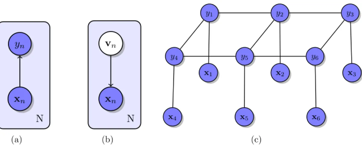
Figure 2.5 Example graphical models : 2.5(a) visualizes logistic regression, used in Chapter 3 and Chapter 4. 2.5(b) visualizes Principal Components Analysis, discussed in Chapter 5. 2.5(c) visualizes a lattice structured CRF, developed further in Chapter 3.

A graphical model consists of a set of nodes, which specify random variables, and edges which specify probabilistic relationships between these variables. Figure (2.3.1) presents three separate graphical models. The first graphical model, Figure (2.5(a)) describes a model in which a variable xn and a variable ynare connected by a directed edge. The “plate notation,” signified by the pale blue node surrounding the two variables indicates the presence of a set of N independent pairs of variables (Spiegelhalter et Lauritzen, 1990).

The directed edge signifies that the random variable yn is conditionally dependent on the random variable xn. In other words, the graphical model depicts a set of N independent conditional distributions p(yn|xn). In this case, both the nodes ynand xnare shaded, indica-ting that they are observed. This means that the model variables are not hidden – the value of both random variables are known. Thus, the conditional distribution of the data is given by QN

n p(yn|xn), by the product rule of probability.

If only the conditional distribution is sought, the model is called discriminative. This is because the model can only be used to determine the probability of a particular y given some input variable x. In contrast, the model can also be trained to optimize the joint probability QN

n p(yn, xn), which is given by QN

n p(yn|xn)p(xn), provided p(xn) is available. In this case, the model is called generative, because it allows for the generation of samples, by sampling an xfrom p(x) and subsequently sampling y from p(y|x). In this thesis, the discriminative model, which will be parameterized to form a particular procedure known as logistic regression, is developed further in both Chapters 3 and Chapter 4.

The second model, shown in Figure (2.5(b)), depicts a probability model in which not all random variables are observed. The model is visually similar to the first, but with two