Calibration of a numerical ionospheric model with EISCAT observations

HAL Id: hal-00329059

https://hal.archives-ouvertes.fr/hal-00329059

Submitted on 1 Jan 1996

HAL is a multi-disciplinary open access archive for the deposit and dissemination of sci-entific research documents, whether they are pub-lished or not. The documents may come from teaching and research institutions in France or abroad, or from public or private research centers.

L’archive ouverte pluridisciplinaire HAL, est destinée au dépôt et à la diffusion de documents scientifiques de niveau recherche, publiés ou non, émanant des établissements d’enseignement et de recherche français ou étrangers, des laboratoires publics ou privés.

Calibration of a numerical ionospheric model with

EISCAT observations

P.-L. Blelly, J. Lilensten, A. Robineau, J. Fontanari, D. Alcaydé

To cite this version:

P.-L. Blelly, J. Lilensten, A. Robineau, J. Fontanari, D. Alcaydé. Calibration of a numerical ionospheric model with EISCAT observations. Annales Geophysicae, European Geosciences Union, 1996, 14 (12), pp.1375-1390. �hal-00329059�

Ann. Geophysicae 14, 1375—1390 (1996) ( EGS — Springer-Verlag 1996

Calibration of a numerical ionospheric model with EISCAT observations

1 C.E.S.R., C.N.R.S./U.P.S. 9 avenue du Colonel Roche, F31029 Toulouse Cedex, France 2 C.E.P.H.A.G., F38492 St Martin d’He`res, France

Received: 1 March 1996/Revised: 10 June 1996/Accepted: 3 July 1996

Abstract. A set of EISCAT UHF and VHF observations is used for calibrating a coupled fluid-kinetic model of the ionosphere. The data gathered in the period 1200— 2400 UT on 24 March 1995 had various intervals of interest for such a calibration. The magnetospheric activ-ity was very low during the afternoon, allowing for a proper examination of a case of quiet ionospheric condi-tions. The radars entered the auroral oval just after 1900 UT: a series of dynamic events probably associated with rapidly moving auroral arcs was observed until after 2200 UT. No attempts were made to model the dynamical behaviour during the 1900—2200 UT period. In contrast, the period 2200—2400 UT was characterised by quite steady precipitation: this latter period was then chosen for calibrating the model during precipitation events. The adjustment of the model on the four primary parameters observed by the radars (namely the electron concentration and temperature and the ion temperature and velocity) needed external inputs (solar fluxes and magnetic activity index) and the adjustments of a neutral atmospheric model in order to reach a good agreement. It is shown that for the quiet ionosphere, only slight adjustments of the neutral atmosphere models are needed. In contrast, ad-justing the observations during the precipitation event requires strong departures from the model, both for the atomic oxygen and hydrogen. However, it is argued that this could well be the result of inadequately representing the vibrational states of N2 during precipitation events, and that these factors have to be considered only as ad hoc corrections.

1 Introduction

For more than half a century, much theoretical work has been carried out to derive the basic transport equations

Correspondence to: P.-L. Blelly

which govern the behaviour of a multispecies plasma (e.g. Chapman and Cowling, 1939; Grad, 1949, 1958; Schunk, 1977). For the specific purpose of studying the ionospheric plasma, beside the main transport terms, large uncertain-ties had to be solved for the collisional processes which involve the neutral species, the thermal-plasma species and the energetic-plasma species (such as precipitating electrons). The choice of these collisional models is impor-tant since, from their definition, the kinetic transport expressions are derived, such as the molecular and am-bipolar diffusion and the thermal conductivity and the viscosity. Various kinds of collision operators were de-veloped [such as the Boltzmann collision integral (Chap-man and Cowling, 1939), the Fokker-Planck collision operator (Rosenbluth et al., 1957; Montgomery and Tid-man, 1964) and charge exchange (Banks and Lewak, 1968)] and theoretical values were determined for the collision frequencies which, for most cases, were found to be consistent with experimental results. However, there still remains some unsolved and important uncertainties: for instance, the O`-O resonant collision frequency re-mains an object of disagreement by a factor of nearly 2 between its theoretical expression as predicted by the most recent studies (Banks and Kockarts, 1973; Pesnell

et al., 1993, 1994) and its indirect measurement in the

ionosphere (Burnside et al., 1987; Salah, 1993; Davis et al., 1995, and references therein).

In addition to the thermal plasma, the ionosphere is characterised by the presence of a significant population of energetic electrons; under the effects of solar EUV radiation, photoelectrons resulting from the ionisation of the neutral atmosphere cascade their energy into the iono-sphere and atmoiono-sphere. At auroral latitudes, in addition to this daytime solar EUV production and energy inputs, energetic electrons precipitating from the magnetosphere downwards to the ionosphere play a role similar to that played by the solar EUV photons; these latter processes can occur anytime, but at a site like EISCAT they occur preferentially when the radar is located under the auroral oval, which occurs mostly during the night. This population

c

Fig. 1. Time/altitude colour plot of ( from top to bottom) the electron concentration, the electron temperature, the ion temperature and the line-of-sight ion velocity, from UHF (top panel) and VHF

(bot-tom panel) French special-program observations. The time

resolu-tion (postintegraresolu-tion) is 5 min. The temporal evoluresolu-tion of electric field resulting from the tristatic UHF radar analysis is added on the UHF panel: the northward component (red) and the eastward com-ponent (green) are plotted in units of mV m~1

of energetic photo- or precipitating-electrons flows through the ambient thermal plasma and is responsible for local energy deposition on the thermal electrons in the lower part of the ionosphere (&100—200 km; Schunk and Nagy, 1978). It was also shown by Blelly and Schunk (1993) and by Blelly and Alcayde´ (1994) that they can contribute to a significant part of the energy transport from the magnetosphere into the topside ionosphere.

These energy inputs are balanced by important local-ised inelastic collisions of the neutral components in the E region (Schunk and Nagy, 1978) or elastic Coulomb collisions in the F region, and then lead to a field-aligned profile of the electron temperature which, due to the electroneutrality of the plasma, controls the field-aligned structure of the ionospheric plasma.

Energy exchange occurs between the energetic-electron population, the thermal-plasma population and the neu-tral atmosphere, which are thereby strongly coupled. A quantitative model of the ionosphere above 100 km then requires accurate modelling of each of these compo-nents.

In the specific case of auroral studies, this implies that electron spectral density structure along the magnetic field line has to be correctly described. Furthermore, energy degradation either in the neutral atmosphere (ionising above about 13 eV, exciting below this limit) or in the thermal electrons (essentially for energies ranging from kB¹e to 10 eV, where kB is the Boltzmann constant and ¹eis the thermal electron temperature) needs to be consis-tently computed. And finally, the energy cooling of the thermal electrons in the neutral atmosphere by rotational, vibrational and fine structure excitation of O, O2 and N2 (the main components of the neutral atmosphere in the E region) has to be accurately determined.

Numerous numerical ionospheric models were de-veloped during the last two decades (Sojka et al., 1981, 1992; Fuller-Rowell et al., 1987; Sojka, 1989; Richmond

et al., 1992; Namgaladze et al., 1996). Most of them were

devoted to global studies of the behaviour of the iono-sphere accounting for its coupling with the thermoiono-sphere and the magnetosphere. However, these models do not consistently solve the transport of the energetic electrons which is crucial for auroral studies. Whenever this is solved, one has to limit the study to local phenomena, since the numerical codes become more and more time consuming. Diloy et al. (1996) presented such a code which solves the thermal part of the ionosphere by a fluid approach (six ions and thermal electrons) and the ener-getic electrons by a kinetic approach. This model is an extension of the Robineau et al. (1996) model which showed its ability quantitatively to represent the F region and topside ionosphere either for steady-state conditions (Robineau et al., 1996) or during dynamical and intermit-tent events (Blelly et al., 1996a). The purpose of this paper is to show how such a model is able to reproduce quanti-tatively the fine ionospheric structures above 100 km for dayside conditions when EUV radiation is the main source of energy and particle production, and for night-side conditions where the precipitating electrons drive the behaviour of the E region and ensure the energy depos-ition within the ionosphere.

In the next section the EISCAT UHF/VHF French special experiment of March 1995 is presented in detail. Section 3 deals with the direct comparison of the numer-ical computation with the experiment; it will be shown that one needs to apply some corrective factors to the model neutral atmosphere for achieving a precise agree-ment between the model and the data. In Sect. 4 the sensitivity of the model to variations imposed by these corrective coefficients is studied. Finally, Sect. 5 draws the main conclusions of the present study.

2 The data

The date chosen for the present study is 24 March 1995. The daily flux of 10.7-cm solar radiation for the previous day was 100 and its three-month average was 81.6; the geomagnetic daily index ap was about 5. On that day, a French EISCAT experiment was run which used both tristatic-UHF and VHF radars.

The UHF radar was operating parallel to the magnetic field and probed the ionosphere between 90 and 600 km. The tristatic volume was located at an altitude of 250 km in the F region. The VHF radar was operating vertically between 280 and 1000 km. The upper limit is imposed by the signal-to-noise ratio, which decreases drastically due to a low ionospheric electron concentration level during the experiment.

Observations of this experiment from 1500 to 2400 UT are gathered in Fig. 1. This plate displays, in coded colours, the temporal evolution of the line-of-sight measurement of the electron concentration (Ne), the electron temperature (¹e), the ion temperature (¹i) and the ion velocity (»i) for the UHF (upper panel) and the VHF (lower panel) radars. Furthermore, the result of the analysis of the tristatic-UHF configuration is plotted as a temporal evolution of the northward (red) and eastward (green) components of the convection electric field. The results from the dyn-asonde placed at the EISCAT Tromso¨ site showed that the calibration constant for the UHF measurements was good within less than 15%, and the UHF can be thereby considered as calibrated for the 24 March. The VHF data were normalised by adjusting the VHF constant until the electron densities around the F2 peak agreed with the calibrated UHF values, and are essentially given as in-dications of the dynamical behaviour north of the Tromsø field line.

From Fig. 1, the experiment can be easily divided in two characteristic periods: the day period between 1430 and 1900 UT and the auroral period between 1900 and 2400 UT.

2.1 The daytime period

As the geomagnetic activity is very low, nothing spectacu-lar is likely to occur during the day, since the EISCAT field of view is located outside of the auroral oval and therefore only a simple diurnal evolution is expected. Indeed the sunset effect is quite visible on both UHF and VHF data, as a decrease in the electron concentration. Since the UHF radar probes both the E and F regions, the sunset effect is well characterised by the upward transla-tion of the Chapman layer correlated with the increase in the solar zenith angle; this effect is particularly visible after 1600 UT. Furthermore, the electron temperature, which strongly depends on solar illumination during this period, decreases with the increasing solar zenith angle and with the diminishing electron concentration, especially after 1700 UT.

The related temporal evolution of the ion temperature is essentially visible on VHF data. Below the UHF upper limit of 600 km, the effects of ion heating by collisions with electrons are masked by the thermalisation of the ions with the neutral species and the daytime variation is therefore weak. Above 600 km (VHF panel), electron-ion collisions are the dominant effects and the ion temper-ature decreases significantly after 1830 UT.

The ion velocities are characteristic of diffusive condi-tions since the magnitudes are a few metres per second, positive above 300 km (F2-peak region) and negative be-low; this situation lasts until 1730 UT. After that time, the velocity turns negative above 300 km: this results from the decrease in the electron temperature and the diminution of the polarisation electric field E4"!(1/eNe)(dpe/ds), where pe"Nek"¹e is the electron gas partial pressure, e is the elementary charge and s is the distance along the line of sight. This feature is mainly visible on the UHF, and less on the VHF due to the larger colour scale. During this period a very low convection electric field is present.

2.2 The auroral period

After 1900 UT, the EISCAT field of view definitely enters the auroral region, characterised by fine structures aligned with the magnetic field. UHF and VHF data display therefore different time-sequences. The horizontal beam separation between the two radars is about 70 km at 300 km; the VHF beam looks vertically and intersects different field lines, at higher L-shells for higher altitudes. Just after 1900 UT, different field-aligned structures are observed on the UHF radar as follows:

d The first occurs at 1910 UT and lasts for 20 min. This structure is associated with a small increase in the electron concentration between 100 and 200 km and an enhancement of the electron temperature above 200 km. No features are visible in the ion temperature and velocity panels. Meanwhile, the convection electric field slightly increases up to 10 mV m~1 and 5 mV m~1 for the north-ward and westnorth-ward components, respectively. This struc-ture seems to correspond to low-energy electron precipita-tion associated with a stable structure coming from the north as seen by the VHF radar: indeed, the structure

occurs first at high altitude and then apparently propa-gates downwards as a result of a north-south drift at a speed of about 400 m s~1.

d At 1940 UT, a sharp increase in the electric field is observed (up to 55 mV m~1 and 20 mV m~1 northward and westward, respectively), with a correlative enhance-ment of the ion temperature at altitudes below 500 km. This is followed, within the time resolution of 5 min, by enhancements of the electron concentration and temper-ature both visible on the UHF panel. This can be inter-preted as being related to a northward electric field at the equatorward edge of an auroral arc (Opgenoorth et al., 1990). As in the previous case, the VHF data shows evidence that this structure was apparently moving through the VHF beam and then enters the UHF one. The four parameters in the VHF panel all show apparent downward propagation with a horizontal beam crossing velocity estimated at 1900 m s~1.

d The third structure starts at 2015 UT and lasts for 20 min. It presents similar UHF features to the previous one in the sense that a sharp increase in the northward component of the electric field (up to 60 mV m~1) fol-lowed by a decrease (down to 20 mV m~1) is observed on the equatorward edge of the structure. Associated with this enhancement, an increase in the ion temperature is observed simultaneously with a sharp decrease in the electron concentration and temperature and an upwelling of the ions. In this case however, evidence of this structure is also seen quite simultaneously on the VHF panel, indic-ating a south-westward moving structure.

d The next event appears at 2110 UT on the UHF radar and lasts until 2200 UT. The structure is associated with an almost constant convection electric field (15 mV m~1 and 5 mV m~1 for southward and westward components, respectively). The event occurs simulta-neously in all four parameters and appears during the expansion phase of a magnetic substorm, as can be seen on the Tromsø magnetogram. The VHF data also show evidence of a moving structure at 2100 UT in all four parameters. The southward beam crossing velocity is esti-mated to be of the order of 1300 m s~1. Enhancement of the vertical velocity up to 400 m s~1 is seen above 500 km. Once the structure is seen on the UHF, a strong and unexplained cooling of the electron temperature is ob-served by the VHF, and the ion temperature is heated below 500 km.

d The onset of the magnetospheric substorm is seen with the electric field turning southwards with a sharp maximum of 35 mV m~1 and the ion temperatures are increased accordingly in both the UHF and VHF data sets. Within the time resolution of the data, this onset is also associated with precipitating electron flux of mean energy around 2 keV (see Sect. 3.2), which then remains roughly constant for about 2 h. Furthermore, as the per-turbation is seen simultaneously by the two radars, and as the electric field is southward, the structure is probably coming from the east, associated with the westward electrojet. During the recovery phase, the southward elec-tric field decreases slowly to 15 mV m~1 until 2220 UT, and then to zero afterwards. After this event, the region probed by the radar is subjected to electron precipitation

patterns, at least until the end of the observation sequence at 2400 UT.

3 Comparison of the numerical model with EISCAT data

The model used in this study has already been extensively presented by Blelly et al. (1996b) and Diloy et al. (1996). It solves, along a magnetic field line, the fluid transport equations for continuity, momentum, temperature and heat flow of six ions (O`, H`, N`, O`

2, N`2 and NO`) and thermal electrons, using an eight-moment truncation scheme [some restrictions in the description of the mo-lecular ions are presented by Diloy et al. (1996)]. More-over, this fluid model is dynamically coupled to a kinetic model which solves the transport along a magnetic field line of suprathermal electrons resulting from either photo-ionisation or precipitation.

Following the studies of Robineau et al. (1996) and Blelly et al. (1996a), who showed the capabilities of such numerical models to reproduce adequately the auroral ionosphere above the F region (200 km) for steady-state conditions and dynamical response to magnetospheric stimuli, the present study is dedicated to the representa-tion of the ionosphere in the E and F regions, starting at 100 km.

In Robineau et al. (1996) a simplified scheme of ion production and energy degradation of the photoelectrons was used, which induces some differences between the data and the model at the lowest altitudes: as a matter of fact, the energy degradation occurs in the region between 150 and 200 km and the ion production at lower altitudes still, between 100 and 150 km, depending on solar condi-tions (solar flux and solar zenith angle). Therefore, it seems interesting to test the ion-production scheme (Lilensten

et al., 1989) and energy degradation scheme

(Lummer-zheim and Lilensten, 1994, and references therein) which are included in the kinetic code.

Furthermore, concerning the dynamical response, field-aligned current, electron heat flow and perpendicular electric-field perturbations were studied by Blelly et al. (1996a), and exhibit different contributions to the dynam-ics of the ionosphere. For a completion of the ionosphere-magnetosphere coupling, precipitation of electrons origin-ating in the magnetosphere needed to be simulated.

Hence, two different periods adapted to the stated goals were chosen. Of the data available, 1500 UT appears to be representative of quiet diurnal conditions. At that time, the solar zenith angle is 80° and the ionosphere is illuminated down to its lowest altitudes. Moreover, as no perturbations occur during the day time period, UHF and VHF data can be combined, assuming that the horizontal variation scales are larger than the beam separation.

Concerning the auroral period, characterised by elec-tron precipitation, the choice is rather more difficult. From 1900 to 2230 UT the preceding discussion showed that the radars observed dynamical structures, rapidly moving through the radar beams. Modelling such features would need to take into account the horizontal transports of the corresponding field lines, which is beyond the scope

of this study. Instead, we have chosen a period of less activity (i.e. after the substorm recovery phase) and deci-ded to model only the UHF-radar observations. Indeed, around 2300 UT, the UHF radar was at the centre of a precipitation period. Albeit that some variations are seen on, for instance, the electron temperatures, they are of small enough amplitude to consider the precipitations as relatively stable. During this period, the sun zenith angle is 109°, and therefore no direct sun production is likely to be observed.

3.1 Ion-composition adjustments

The determination of the electron and ion temperature is highly dependent on the value of the composition para-meter p"[O`]:Ne. As the UHF standard analysis pro-gram uses a constant statistical O` composition model to infer the values of ¹i and ¹e from the incoherent spec-trum, some differences between the estimated and the true values are likely to occur in the region of transition from molecular ions to atomic ions (around 200 km). To com-pare the results from the simulation to the measurements, the composition parameter should be the same. For this purpose, in addition to the results produced by the stan-dard EISCAT-analysis routine, the data were processed with the ion-composition profile provided by the numer-ical model. In the following, these two evaluations of ¹e and ¹i profiles will be discussed together with the composition profiles. The same result is obtained by scal-ing the ¹e and ¹i profiles usscal-ing correction formulas (Wal-dteufel, 1971).

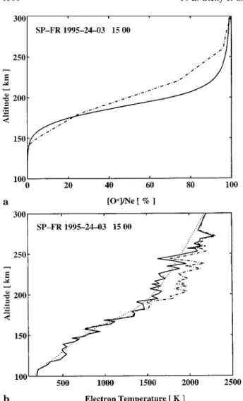
Figure 2a gives a comparison between the standard composition and the modelled one at 1500 UT. The transition altitude is 200 km in the standard analysis model and 190 km in the simulation. The shapes are similar but the slopes around the transition altitude are slightly different. Figure 2b displays the altitude profile of the electron temperature. When the results of the standard analysis are compared to the numerical model, large dis-crepancies appear in the transition region between 180 and 230 km. If the numerical model composition profile is used instead, most of the discrepancies are removed, as shown by Fig. 2b. One claims, therefore, that in the pres-ent case, the numerical composition model is likely much better than the statistical one, as it allows us to reconcile observed and modelled electron temperatures (and ion temperatures as well, not shown here). In the following, comparisons will be made with these composition-adjusted temperatures.

3.2 Neutral-atmosphere adjustments

Robineau et al. (1996) explained difficulties which exist when using global indices such as solar flux F10.7 and geomagnetic index ap to characterise external sources. Moreover, the use of statistical models, such as the MSIS-90 neutral-atmosphere (Hedin, 1991) and the HWM-90 neutral-wind (Hedin et al., 1991) models gives rise to the critical problem of using averaged values for

Fig. 2a, b. Vertical profiles at 1500 UT, between 100 and 300 km, of a [O`]:Ne parameter for standard statistical model (dot-dashed

line) and the result of the simulation ( full line); b electron

temper-ature calculated by the standard analysis (dot-dashed line), corrected electron temperature ( full line) and electron temperature resulting from the simulation (dotted line)

solar and geomagnetic activity rather than instantaneous ones. Blelly et al. (1992) showed that, even for quiet condi-tions, values inferred from the data can either be in a fairly good agreement with the model (e.g. atomic oxygen, exo-spheric temperature), or present large discrepancies (neu-tral atomic hydrogen for example). Thus the numerical model includes correction factors on the concentrations derived from the statistical models for the atomic oxygen (CO), the atomic hydrogen (CH), and the atomic nitrogen and the molecular (N2 and O2) components (CM). In addition, deviations in the exospheric neutral temperature (d¹inf) and neutral meridional wind (dºinf) are allowed. The sensitivity of the numerical model to such adjustment factors and deviations will be discussed in Sect. 4.

Finally, as already reported by Blelly and Schunk (1993) and Diloy et al. (1996), such modelling requires a topside boundary condition for the electron heat flow, which characterises the energy input from the magneto-sphere. As a matter of fact, such a condition should be

provided by the kinetic part of the model, since it corre-sponds to energetic electrons flowing down into the iono-sphere. However, the coupling between the fluid and the kinetic part is not yet adapted to such a boundary condi-tion, and therefore a topside electron heat-flow condition is imposed to the model, so that the modelled electron-temperature profile follows as closely as possible the data profile above 500 km.

3.3 The daytime period

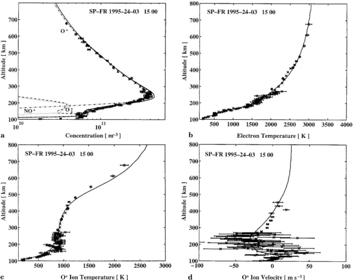
Figure 3 gives the comparison between the model and the data profiles at 1500 UT. UHF data are plotted with crosses and VHF data with circles; error bars are superim-posed onto the data. The adjustment coefficients for the neutral models are given in Table 1. This set of parameters allows for an overall agreement between the model and the data.

Concerning the electron concentration (Fig. 3a), the main features are well reproduced. The E region is domin-ated by O`

2 ions with a peak density of 7]1010 m~3 located at 120 km, in agreement with the UHF alternat-ing-code results. The modelled F2 peak of 4.5]1011 m~3 amplitude at 220 km is about 10% higher than the UHF measurement, with a peak correctly positioned. Between the E and F2 peaks, the ionospheric structure closely follows the data set; between 150 and 200 km, O`

2 and NO` have similar concentration levels and represent more than 50% of the ion concentration, O` being the major species above. This transition altitude between the molecular and the atomic ions corresponds to the transition altitude that Lathuille`re and Pibaret (1992) found for winter. The reaction:

O`#N2PNO`#N, (1)

which involves vibrationally excited N2, is included in the model with the reaction rate fitted by St Maurice and Torr (1978) and is expressed as a function of the neutral temper-ature and the O` temperature. However, this rate should depend on the vibrational temperature of N2 (Pavlov, 1988, 1993, 1994), which may be higher than the neutral one (Newton et al., 1974), and may therefore be much more efficient in recombining O`. For diurnal winter and solar minimum conditions Richards and Torr (1986) and Ennis et al. (1995) show that this effect is not significant and does not alter the F2-peak region. However, the inverse occurs for summer and high solar conditions: the F2 peak can be reduced by a factor of 2 due to the increasing efficiency of reaction (1). Similar effects may be observed when electron precipitation occurs because en-hanced, vibrationally excited N2 is likely to be produced by electron impact.

The correct description of the field-aligned distribution of the electron-concentration data shows that the O` production is properly modelled. As this production re-sults from the photoionisation of atomic oxygen, the cor-rection suggested for [O] in Table 1 is probably indicative of reality.

Fig. 3a–d. Comparison between SP-FR experiment and the model-ling at 1500 UT; vertical VHF data profiles (circles) and field-aligned UHF data profiles (crosses) with the error bars compared to the result of the simulation (straight line) for a electron concentration

O` (dot-dashed line), NO` (dotted line) and O`<sub>2</sub> (dashed line) concen-tration profiles are plotted to give some indication on the composi-tion; b electron temperature; c O` ion temperature; d O` ion velocity (VHF data are not plotted)

Table 1. List of adjustment parameters at 1500 UT for atomic oxygen O (CO), atomic hydrogen H (CH), atomic nitrogen and molecular components O2 and N2 (CM), departure from exospheric temperature (d¹inf) and exospheric meridional wind (dºinf) and topside electron heat flow (positive upward)

CO 0.9 CH 1 CM 1.3 d¹inf [K] !60 dºinf [ms~1] !90 qtop_e [lW m~2] !0.3

The altitude of the F2 peak and the scale height of the electrons above the peak are controlled by diffusion of O` and chemical loss through the charge-exchange reaction: O`#HQPO#H`. (2) As can be seen in Fig. 3a, the modelled electron scale height above the F2 peak corresponds to the measurement

up to about 700 km. In this figure, the VHF data have been calibrated using the UHF measurement around 280 km (long pulse). The diffusion is strongly related to the neutral atmosphere (essentially O) through ion-neu-tral collisions and meridional neuion-neu-tral wind (which can translate the F layer in altitude), and the chemistry is related to the neutral atmosphere (O and H) through chemical equilibrium resulting from reaction (1). There-fore, such an agreement between model and data charac-terises a good estimation of the O`-O collision frequency, the meridional wind, the [H] : [O] ratio and thereby [H]. Figure 3b gives the result of the simulation for the electron-temperature profile. The thermal structure is im-posed at the lowest altitudes (below &200 km) by local processes: balance between energy transfer from the suprathermal electrons (of energy around 10 eV) to the thermal electrons and inelastic cooling of the thermal electrons by the neutral species (mainly O2, N2 and O) through vibrational and rotational excitation of O2 and N2 and fine structure excitation of O (Schunk and Nagy, 1978), and by elastic electron-ion collisions above 300 km

(F2 peak). At higher altitudes (above &400 km), thermal conduction controls the evolution of the electron-temper-ature gradients through energy exchange with the mag-netosphere (Blelly and Schunk, 1993; Blelly and Alcayde´, 1994); the structure is then determined by the topside-electron-heat-flow condition. In the mid-range altitude, the equilibrium is a mixture of local energy transfer and energy transport. The fact that the structure is well repro-duced at all altitudes implies that the relative weight of heating and cooling sources and energy transport are correctly modelled.

The heating source is a direct byproduct of the kinetic part of the model and strongly depends on the neutral atmosphere; so is the cooling sink, which is directly related to the neutral-atmosphere concentrations.

At low altitudes (below 150 km), the cooling due to rotational excitation represents more than 50% of the cooling mechanism, and the electron-temperature gradi-ent is mainly due to the small scale height of the neutral components O2 and N2. It decreases down to 40% above 200 km, while fine structure excitation of O increases up to 30%. Between 200 and 300 km, the vibrational excita-tion represents 20% for N2 and 10% for O2. The mecha-nism of vibrational excitation is rather difficult to handle, especially for N2, since it strongly depends on the concen-tration level of vibrationally excited N2 which results from an important number of chemical sources (Richards et al., 1986). Stubbe and Varnum (1972) have derived an expres-sion for this cooling mechanism, but since then, new calculation of the total cross-section may increase its efficiency by up to 3 times (Richards et al., 1986). For fine structure excitation of O, the reverse may occur: Carlson and Mantas (1982) have found that the cooling expression given by Hoegy (1976) represents in fact an upper limit, and the actual rate may be much smaller. For that time, including these changes in the computation of the cooling rate would modify the global rate by less than 20%: it would become stronger in the 200—300 km range due to an enhanced vibrational excitation of N2. If the factor was 2 for N2, there will be no significant change between 200 and 300 km.

For an electron-concentration profile with a peak at 250 km and a heating rate with a peak at 200 km, the heating rate per electron exhibits a sharp layer maxi-mising at 180 km. This explains the change in concavity around 160 km which is quite visible in Fig. 2b. Below this altitude, the heating increases with altitude, and the bal-ance between the heating and the cooling by rotational excitation can only be ensured by an important temper-ature departure between the electrons and the neutrals. The sharp layer of the heating rate per electron around 190 km imposes an enhancement of the electron temper-ature around this altitude, inducing a concavity change around 160 km. Above 200 km, the cooling by vibrational excitation becomes very efficient while the heating rate per electron is decreasing; thereby, a change is imposed in the electron-temperature gradient, inducing another concav-ity change around 200 km.

Around 300 km, the fine structure excitation of O and the elastic collisions between electrons and ions become the two predominant sinks of electron cooling which

contribute significantly to balance the energy input from the magnetosphere. The electron heat flow exhibits a min-imum around 320 km, which represents the limit of influ-ence between local processes and field-aligned transport. This minimum corresponds to a concavity change in the electron-temperature gradient: below 320 km, the temper-ature evolution is controlled by the local cooling; above 320 km it is controlled by the heat-flow altitude depend-ence, which, due to the high mobility of the electrons, follows a divergence free law (Blelly and Schunk, 1993). These successive gradient breaks are characteristic of the influence of different terms contributing to the overall electron-temperature structure. The close agreement be-tween the data and the model is an indication that these features are quite well reproduced and thus that the differ-ent contributions are correctly modelled.

The ion temperature structure (Fig. 3c) is much more simple. At low altitude (below 300 km) and without con-vection electric fields, the profile is imposed by the neutral temperature; at high altitude (above 800 km) it is imposed by energy transfer from thermal electrons through ion-electron Coulomb collisions. Between 300 and 800 km, the profile results from the balance between cooling of O` ions by atomic oxygen through resonant collisions and heating by thermal electrons; these features allow for a realistic determination of the exospheric neutral temper-ature (Blelly et al., 1992), or its deviation from the exo-spheric-temperature model (!90 K in this case). The structure between 300 and 800 km is then related to the atomic-oxygen content within this altitude range and to the O`-O collision cross-section. In this study, the O`-O collision cross-section given by Banks and Kockarts (1973) is multiplied by the so-called Burnside factor 1.7 (Burnside et al., 1987; Salah, 1993). With atomic oxygen calibrated through the electron concentration pro-file, Fig. 3c shows that the chosen correction factor is well adapted to describe the overall ion temperature evolution. Figure 3d presents the results for field-aligned vel-ocities. The VHF velocity data have been removed be-cause they are not field-aligned as the UHF data are. The meridional wind has been adjusted (!60 m s~1) so that the ion velocity below 150 km corresponds to that measurement. The result exhibits a diffusion regime with velocities below 30 m s~1 at 800 km. Due to a very noisy measurement of the velocity with the alternating code below 300 km, it is rather hard to compare the model and the data. Nevertheless, around 200 km, the general trend of the measurement is to reach a minimum value of about !40 m s~1 at 200 km, just below the F2 peak. Above 200 km, diffusion drives the velocity evolution. It becomes positive above 400 km and the profile of the simulation is well in agreement with long-pulse measurements up to 450 km.

We get an overall good agreement between the model and the data with a reduced number of parameters. Com-pared to the complexity of the different mechanisms in-volved, the importance of which varies significantly with altitude, we may be confident of the values of these para-meters. Therefore, these values should be representative of the atmospheric conditions for 24 March and should not change notably during the day.

Table 2. List of adjustment parameters at 2300 UT for atomic oxygen O (CO), atomic hydrogen H (CH), atomic nitrogen and molecular components O2 and N2 (CM), departure from exospheric temperature (d¹inf) and exospheric meridional wind (dºinf) and topside electron heat flow (positive upward)

CO 0.5 CH 6 CM 1.3 d¹inf [K] 30 dºinf [ms~1] 0 qtop_e [lW m~2] !1.5

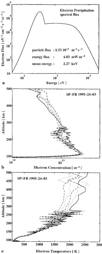
Fig. 4. a Spectral density of the flux of precipitating electrons used to adjust the model at 2300 UT. The low-energy part is a Maxwel-lian shaped function with a maximum reached at 350 eV. The high-energy part is a complex power-law function with a quasi-constant function between 500 eV and 4 keV and an asymptotic branch varying as the fifth power of the inverse of the energy above 4 keV; b the 5-min-integrated profiles of the electron concentration for the 20-min period centered on 2300 UT (the full line corres-ponds to 2300 UT, the dash-dotted lines to the period before and the dotted lines to the period after); c the same for the electron temperature

3.4 The auroral period

The adjustments for this time are given in Table 2. As can be noticed, a significant change in O and H correction coefficients (compared to 1500 UT) was needed to get a good correlation. It has to be mentioned that since the ionosphere has been perturbed for about 4 h, the neutral atmosphere is likely to be affected by the energy input to the ionosphere from the magnetosphere. The fact is that the evolution of the exospheric temperature between 1500 and 2300 UT is about 40 K as given by the empirical MSIS-90 model. In this study, we find a lower temper-ature during the day and a higher one at 2300 UT, with a variation amplitude of 130 K. This may indicate that successive perturbations have induced a slight enhance-ment of the neutral temperature during the period 1500—2300 UT. This may also indicate that the neutral components have been affected, but such an amplitude in the observed atomic oxygen and hydrogen are question-able, and we use these correction factors as adhoc para-meters for the calibration. The null correction found for the meridional wind means that the wind inferred by the HWM model, i.e. 210 m s~1, is adequate for representing the observations. No simultaneous FPI observations were available for the considered period, but such an amplitude for the meridional wind is a very reasonable value when compared to the ‘mean meridional wind’ for most of the night-time periods of March (Aruliah et al., 1991a, b, 1996; Rees, 1995).

With the corrected atmosphere, we needed to impose a specific spectral flux (intensity) of electrons precipitating from the magnetosphere. The spectral density is plotted in Fig. 4a. The spectrum is obtained with the superimposi-tion of two spectra. The first is a Maxwellian-shaped spectrum with an energy width of 350 eV. It corresponds to low-energy electron precipitation, which plays a role at altitudes above 200 km due to the atmospheric scattering depth imposed by the neutral atmosphere (Rees, 1989 and references therein). The high-energy spectrum is a complex power law characterised by a plateau between 500 eV and 4 keV and an asymptotic branch which varies as the fifth power of the inverse of the energy. The total particle flux is 1.3]1013 m~2 s~1 and corresponds to an energy flux of about 5 mW m~2 into the ionosphere. The choice for the spectral flux is governed by the vertical structure of the electron profile. However, the shape is well in agreement with typical auroral intensities measured on-board satellites, especially with this double-humped

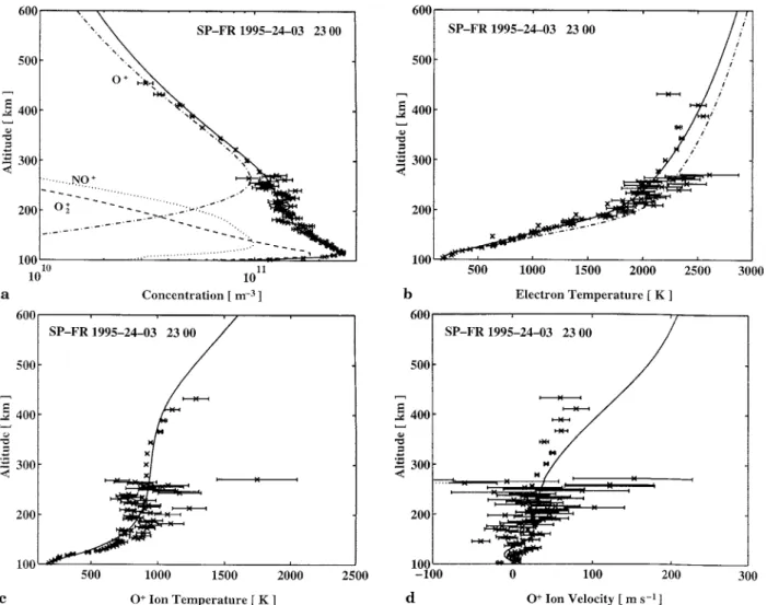
Fig. 5a–d. Comparison between SP-FR experiment and the model-ling at 2300 UT; the result of the simulation (straight line) compared to field-aligned UHF data profiles (crosses) with the error bars for a electron concentration O` (dot-dashed line), NO` (dotted line) and O`₂(dashed line) concentration profiles are plotted to give some

indication on the composition; b electron temperature (dot-dashed

line corresponds to standard vibration excitation of N2 and the full line to a double vibration excitation of N2); c O`-ion temperature;

d O`-ion velocity

function. Fig. 4b, c displays altitude profiles of the electron concentration and temperature at 2300 UT and $10 min apart; it shows that the electron production and heating in the E region was stable (a few percent scattering at the E peak). The energy-flux spectrum given in Fig. 4a is therefore characteristic of this period apart from the very low energy part which produced an excess of production and larger temperatures between 200 and 250 km. This latter effect was considered interesting to simulate for testing the ability of modelling the very low energy (below 300-eV) production and heating of the precipitating elec-trons.

Figure 5a presents the simulated electron profile com-pared to the UHF measurement. The characteristic of the structure is a pronounced E region with a peak amplitude of 2.6]1011 m~3 located at 115 km. The F2 peak is not clearly visible because of the precipitation but is located around 280 km. With the spectral flux chosen, the electron density structure is quite well reproduced.

The asymptotic branch of the spectral flux has been chosen so that the evolution of the electron concentration below the E-region peak follows the data: the peak corre-sponds to a 4-keV precipitating electron beam (Kirkwood and Osepian, 1995). The effect of the precipitating elec-trons in that altitude range is mainly the production of O`

2. However, the production of NO` by the chemical reaction:

O`

2#N2PNO`#NO (3) is responsible for the significant presence of NO` around 120 km. Above 120 km, NO` becomes the major species up to about 180 km; its diffusion is compensated by its production through chemical recombination of Eq. 1. As already mentioned, this recombination mechanism is highly dependent on the vibrational state of the molecular component N2. Newton et al. (1974) showed that in stable auroral red arcs, electron impact may produce an impor-tant amount of vibrationally excited nitrogen and thereby

increase the reaction rate by a factor of as large as 8. Richards and Torr (1986) showed that for enhanced vibra-tional excitation of N2 (occurring in summer during solar maximum) the F2-peak concentration can be reduced by a factor of 2. This effect was confirmed by Ennis et al. (1995), who showed that this reduction effect is not signifi-cant in winter for suprathermal electrons resulting from ionisation of the neutral atmosphere by solar radiations. The true reaction rate is rather hard to infer when precipitations occur: St Maurice and Torr (1978) mention that a small amount of excited N2 could lead to a large increase in this rate, resulting in a drastic depletion of the F layer.

As already mentioned, we have significantly to change the correction coefficients on both atomic oxygen and hydrogen in order to adjust the model to the data. If we assume that the neutral atmospheric model has to be adjusted, this adjustment is likely to be roughly constant for a given day, even if the atmosphere is slightly pertur-bed by the ionosphere. Thereby, CO should vary around 0.9 and CH around 1. The fact that CO"0.5 and CH"6 are necessary to adjust the F2 peak and the diffusion region means that the ion production due to precipitation is too large when compared with the losses by chemical reactions and diffusion. However, an alternative mecha-nism implying N2 vibrational states, could also be in-voked, thus avoiding such large changes in the correction factors CO and CH.<sub>The point is that the maximum of the O` production</sub> rate occurs at an altitude below 200 km and is due to the high-energy tail of the precipitating electron spectrum. Yet, this high-energy part was adjusted in order to repro-duce the E region: thus, we need either to rerepro-duce the atomic oxygen content or to increase the losses by chem-ical reactions. The choice was made for a change in the oxygen content and an enhancement of O` losses by the charge-exchange reaction (4). However, a reduction in the F2 peak by a factor of 2 could alternatively be obtained with an enhancement of the vibrational state of N2 (Richards and Torr, 1986). Newton et al. (1974) showed that for auroral red arcs, the decrease in the electron content within the arc was mainly due to electron precipitation which excites the different vibrational levels of N2 and significantly increases the rate of recombination through reaction (4). Such a mechanism would result in an upward translation of the P2 peak and of the transition altitude, but the concentration profile would change es-sentially in the 150—250-km altitude range, where the measurements are noisy enough to allow some flexibility in the adjustment.

This mechanism could also explain the electron tem-perature profile discrepancies plotted in Fig. 5b. The dot-dashed line represents the electron temperature obtained with the cooling term by vibrational excitation of N2 as given by Stubbe and Varnum (1972); the full line corres-ponds to an increase by a factor 1.9 in this cooling term. As can be easily seen, this correction allows for a better agreement of the modelled temperature below 200 km: differences of about 300 K between the two modelled electron temperatures are found around 180 km. This correction factor is consistent with that suggested by

Richards et al. (1986). In the expression derived by Stubbe and Varnum (1972), the various excited states are assumed to have constant statistical weights, and the neutral temperature is used to characterise the excited neutral population. If one of these assumptions fails because of electron-precipitation impact, the cooling term may change significantly.

This alternative effect resulting from enhanced N2 vibration would reduce significantly the need for chang-ing the CO and CH coefficients. It would also explain both the Ne and ¹e profiles. However, taking it into account would require a full simulation of N2 vibrational states, which is beyond the scope of the present study. Hence, the CO and CH factors are only to be taken as ad hoc factors.

As can be noticed, the value of topside electron heat flow used at 2300 UT (!1.5lW m~2) is five times the value used at 1500 UT (!0.3lW m~2), in order to account for the 5 mW m~2 energy flux input into the ionosphere from electron precipitations of magneto-spheric origin.

Figure 5c presents the results for O` temperature. Despite the noisy character of the measurement, this fig-ure shows excellent agreement between model and data. With respect to the velocity (Fig. 5d), one can see that the model results are slightly higher than the measurement above the F2 peak. This is mainly due to a reduced O`-O collision frequency (imposed by the reduction of atomic oxygen) and then an enhanced molecular-diffusion coeffic-ient. Moreover, more atomic hydrogen components in-duce more H` ions and more O` ions upflowing. The difference between the model and the data could be re-duced if the mechanism which depletes the F2 region is the recombination equation (4), because we could have a lar-ger neutral atomic oxygen concentration. This again goes in favour of the N2 vibrational scheme.

4 Sensitivity to the adjustment coefficients

Each calibration parameter is more or less dependent on the others for the overall adjustment. By determining the sensitivity of the model to each parameter, we can obtain strong indications of the quality of the adjustment. Some of the parameters are simpler to adjust than others be-cause they can easily be decoupled from the others: d¹inf,

dºinf and qtope . On the other hand, the concentration adjustment factors are interconnected. Therefore, we deci-ded to test the sensitivity of the coefficients to molecular components (CM), atomic oxygen (CO) and atomic hydro-gen (CH). Moreover, as the O`-O collision frequency is an important feature of the ionosphere-atmosphere coupling above the F region, we also tested the sensitivity to the Burnside factor.

The evaluation is made for the daytime period; for each parameter, the simulation corresponding to the standard value is compared to the results obtained with two other values of the parameter, significantly different from the standard one and bracketing it (except for the Burnside factor).

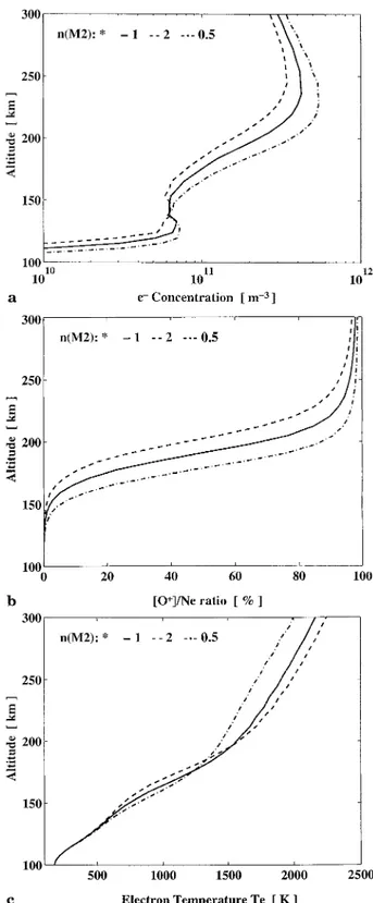
Fig. 6a–c. Effect, in the altitude range of interest, of the neutral molecular atmosphere (O2 and N2) on the profiles of a electron concentration, b O` composition parameter and c electron tem-perature. The full line corresponds to the standard adjustment, the

dashed line to molecular component concentrations multiplied by

2 and the dot-dashed line to molecular components concentrations divided by 2

4.1 Neutral molecular components

The adjustment factor for the quiet daytime period was found to be 1.3 (Table 1). The profiles of the plasma parameters which are most affected by a variation of the factor between 0.5 and 2 are shown in Fig. 6: these are the electron concentration, the composition and the electron temperature.

For the electron concentration, the main effects of reducing the neutral molecular concentrations by a factor of 2 (CM"0.5) are to reduce the recombination of O` through reaction (6) and thus to increase the F2-peak electron concentrations. Also, as the optical depth is glo-bally reduced, the same production is found at lower heights and thus the layer is shifted to lower altitudes.

In the E region, decrease in the neutral concentration is overcompensated by the fact that less solar EUV energy has been absorbed and the resulting electron concentra-tions (mainly O2` and NO`) are surprisingly increased significantly.

Globally, the O` ionosphere is shifted down by 10 km, as shown by the [O`]:Ne ratio. The corresponding elec-tron temperatures are lower in the F region, due to the increase in the electron concentration for the same energy inputs; but in the E and F1 regions the effects are quite negligible. Increasing instead the molecular concentra-tions would have the reverse effects (see Fig. 6). We can conclude then that the molecular species affect the elec-tron concentration at all altitudes, even in the F region.

4.2 Neutral atomic oxygen

Figure 7 shows the effects of changing the atomic oxygen concentration from the MSIS-90 model. As anticipated, this has an impact essentially at F-region heights where atomic oxygen is the major constituent, while at E-region altitudes, where the molecular dominates, the effects are very small.

Increasing the atomic oxygen concentration results in an increase in the O` production rate and thereby in the F2-peak concentration level, the altitude of which is trans-lated upwards (Fig. 7a). The O` production in the E re-gion is more important, lowering by then the transition region between the molecular and atomic ions. Also, the increase in the neutral atomic oxygen concentration im-plies an enhancement of the collisions of electrons and ions with neutrals: both the electron and ion temperature are therefore reduced in this process (Fig. 7c, d). The electron temperature is strongly reduced in the F2-peak region, because for the same energy input, more electrons are created and the cooling by fine structure excitation of atomic oxygen and electron-ion elastic collisions are much more important due to higher electron, O` and atomic oxygen concentrations. The change in the elec-tron-ion coupling is evidenced in Fig. 7e where the ion-temperature gradient is shown to be decreased and its peak occurs at greater heights. The altitude of transition between the energy cooling of O` by atomic oxygen and energy heating of O` by electrons is characterised by a change in the slope of the temperature (Fig. 7d) and

Fig. 7a–e. Effect, in the altitude range of interest, of the ato-mic oxygen on the profiles of a electron concentration, b O` composition parameter, c electron temperature, d O` ion temperature and e O` ion-temperature gradient. The full line corresponds to the standard adjustment, the dashed line to atomic oxygen concentration multiplied by 2 and the dot-dashed

line to atomic oxygen concentration divided by 2

therefore by a maximum in the temperature gradient (Fig. 7e). It can be easily seen that when the neutral concentration increases, the altitude of transition is trans-lated significantly upwards: in other words, the ions are cooled by the neutrals at higher altitudes.

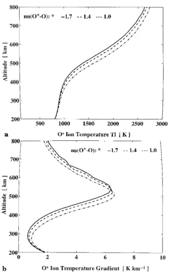
4.3 Burnside factor

The effects of the Burnside factor on the O`-O collision cross-section were tested by assuming values ranging be-tween 1 and 1.7. The latter was considered as the nominal

Fig. 8a, b. Effect, in the altitude range of interest, of the Burnside correction factor to O`-O collision cross-section on the profiles of a O` ion temperature and b O` ion temperature gradient. The full

line corresponds to the standard admitted value of 1.7 (Salah, 1993),

the dashed line to the value of 1.4 as suggested by Davis et al. (1995) and the dot-dashed line to the collision cross-section initially sugges-ted by Banks and Kockarts (1973)

Fig. 9. Effect, in the altitude range of interest, of the atomic hydro-gen on the O`-ion-concentration profile. The full line corresponds to the standard adjustment, the dashed line to atomic-hydrogen con-centration multiplied by 5 and the dot-dashed line to atomic-hydro-gen concentration divided by 5

value in the present study, but may well be revised for future works, following the CEDAR-1996 meeting recom-mendations. It is therefore interesting to estimate the effects of changes in its value.

Reducing this factor to 1 has practically no effect on the electron concentration and temperature. Concerning the O` temperature, reducing the correction on lO

`-Oby 1.7 (Fig. 8a, b) has consequences similar to those obtained with a reduction in the atomic-oxygen concentration (Fig. 7d, e): decreasing the Burnside factor is equivalent to reducing the cooling of the ions by the neutrals. Thus, the ion temperature profile alone does not allow for a distinc-tion between the two processes. They can only be separ-ated by using the electron concentration and temperature.

4.4 Neutral atomic hydrogen

These effects are shown in Fig. 9 for the O` concentration profile. The main effect of increasing the atomic hydrogen

concentration is to enhance the efficiency of the O`-H charge-exchange reaction (4), and thus to reduce the O` concentration in the F region and above. However, this effect only becomes sensitive for large increases (a factor of 5 in the present case) in the atomic hydrogen concentration. On the other hand, if one reduces the minor hydrogen atom concentration, it becomes negli-gible and almost no effects are observed (see Fig. 9). Nevertheless, one can notice the O` ion scale height depends on the neutral atomic hydrogen. The fact is that H` becomes more important with an increasing coeffic-ient. The composition of the plasma is then significantly altered and so is the plasma pressure. If O` were the only ions in the plasma, they would be in a diffusive equilib-rium with the plasma scale height, as a result of the polarisation of the plasma. Due to an enhanced propor-tion of H`, they are diffusing with a smaller scale height than the plasma one, and a higher velocity, as mentioned in Sect. 3.2.

4.5 Summary

To conclude the study of sensitivity, we can say that the concentration adjustment parameters have different char-acteristic influences on the ionospheric structure: CM sig-nificantly alters the electron concentration at all altitudes,

CO the electron temperature in the F region and CH the

electron scale height above the F region. Then, the overall adjustment suggests that it is best to estimate these para-meters in the region of most importance, i.e. CM in the E region, CO in the F region and CH above the F region. Then fine tuning must be done in order to reproduce the transition region (essentially the molecular to atomic ion transition region). This procedure shows that good confi-dence can be placed in the adjustment of the correction factors.

5 Conclusion

The model used in the present study is time dependent and is thus well suited for studies of temporal evolution of the ionosphere. However, in the present version, we did not consider the convection transport of magnetic field lines in the auroral and polar regions. The model is therefore limited to regions where the convection is not a predomi-nant feature of the ionospheric dynamics. Thus, we did not attempt to calibrate the model to the data during the events between 1900 and 2200 UT, for which convection and dynamics are predominant features. We limited our study to periods characterised by some stability of the external sources, namely around 1500 UT and 2300 UT.

The period around 1500 UT is representative of a dy-namical equilibrium of the daytime ionosphere. It was a quiet period for which only minor corrections on the neutral atmosphere were necessary. However, an impor-tant feature found was the need for an adjustment of the ion composition in order to reconcile model results and data. With such corrections, we reached a high degree of accuracy in the description of the electron concentration and temperature and ion temperature. The diffusive be-haviour of O` is also quantitatively reproduced in the chemical region (F1 region), where neutral atmosphere controls the dynamics, and in the region above the F2 peak, where the structure is controlled by plasma neutrality and ambipolar flow.

The neutral atmosphere parameter adjustment, used to calibrate the model, appears to be a more sophisticated extension of previous methods developed to infer neutral-atmosphere parameters from incoherent-scatter data (Vasseur, 1969; Bauer et al., 1970; Blelly et al., 1992). In this case the entire data set is used for an overall adjust-ment.

The 2300 UT period is at the centre of a stable electron precipitation event with a weak convection electric field. The events before 2300 UT have strongly perturbed the ionosphere for quite a long time (about 4 h), and the neutral atmosphere is likely to be affected; more-over, the energetic precipitation acts on the neutral atmosphere through electron impact. However, the inferred adjustment parameters for the neutral atmo-sphere, which are much larger for atomic oxygen and hydrogen concentration than during the quiet period, are unreasonable.

An explanation may be found in the role that excited states of N2 can play in the chemical process: any en-hancement of the amount of vibrationally excited N2 would significantly increase the recombination of O` and would thereby reduce drastically the O` concen-tration in the F region, as suggested by the data. The electron temperature profile observed between 150 and 200 km is a further indication of the likely increased influ-ence of the vibrational excited levels of N2 on the iono-spheric structure below 300 km.

This shows that adjusting electron precipitation on the neutral concentration profile alone may produce erron-eous results if such effects are not taken into account either explicitly by quantifying the vibrational levels or in an ad hoc manner, as has been done in the present study.

With this precaution in mind, the spectral density flux of the precipitating electrons has been derived in order to reproduce both the electron concentration and temper-ature profiles, while accounting for the corrections on the neutral atmosphere. The adjustment of the model on the data, using the calculated electron flux is quite as good as for the quiet day period.

This work has shown the capability, by comparing model and data, of revealing inaccuracies or deficiencies in the modelled state of the atmosphere, of the ionospheric composition and in some reaction rates. Therefore, this study stresses some critical aeronomic problems which need to be taken into account in order to reach a quantit-ative level in modelling the auroral ionosphere. This may be more crucial in the polar region: indeed, above 200 km, vibrationally excited N2 has long-enough diffusion times to be transported large horizontal distances by convection before quenching with O` ions (Pavlov, 1993).

Acknowledgements. This research was supported by the GdR

PLASMAE program of CNRS. The authors are indebted to Dr. Mike Rietveld who provided EISCAT Dynasonde data for calib-ration purposes, and to Dr. David Rees who provided mean meridi-onal wind FPI estimates for March periods. The authors thank the EISCAT Director and his staff for their assistance in running EIS-CAT experiments. EISEIS-CAT is an International Association sup-ported by the Research Councils of Finland (SA), France (CNRS), Federal Republic of Germany (MPG), Japan (NIPR), Norway (NAVF), Sweden (NFR) and United Kingdom (PPARC).

The Editor-in-Chief thanks C. Fesen and A. D. Aylward for their help in evaluating this paper.

References

Aruliah, A. L., D. Rees, and T. J. Fuller-Rowel, The Combined effect of Solar and Geomagnetic Activity on High-Latitude Thermo-spheric Neutral Winds, J. Atmos. ¹err. Phys., 53, 467—483, 1991a.

Aruliah, A. L., D. Rees, and A. Steen, Seasonal and Solar Cycle Variations in High-Latitude Thermospheric Winds, Geophys.

Res. ¸ett., 18, 1983—1986, 1991b.

Aruliah, A. L., A. D. Farmer, D. Rees, and U. Brandstrom, The Seasonal Behaviour of High-Latitude Thermospheric Winds and Plasma Velocities Observed Over One Solar Cycle, J. Geophys.

Res., in press, 1996.

Banks, P. M., and G. Kockarts, Aeronomy, Academic Press, New-York, 1973.

Banks, P. M., and G. J. Lewak, Ion velocity distributions in a par-tially ionised plasma, Phys. Fluids, 11, 804—810, 1968.

Bauer, P., P. Waldteufel, and D. Alcayde{ , Diurnal variations of the atomic oxygen density and temperature determined from inco-herent scatter measurements in the ionospheric F-region, J.

Geo-phys. Res., 75, 4825—4832, 1970.

Blelly, P.-L., and D. Alcayde{ , Electron heat flow in the auroral ionosphere inferred from EISCAT-VHF observations, J.

Geo-phys. Res., 99, 13181—13188, 1994.

Blelly, P.-L., and R. W. Schunk, A comparative study of the time-dependent standard 8-, 13- and 16-moment transport formula-tions of the polar wind, Ann. Geophysicae, 11, 443—469, 1993. Blelly, P.-L., J. Fontanari, D. Alcayde{ , J. Wu, M. Blanc, and T. L.

Hansen, Observations of the structure and vertical transport of the polar upper ionosphere with the EISCAT-VHF radar. 3. Topside neutral composition and quiet-time temperature, Ann.

Geophysicae, 10, 394—406, 1992.

Blelly, P.-L., A. Robineau, and D. Alcayde{ , Numerical modelling of sporadic ion outflow events above EISCAT, J. Atmos. ¹err.

Blelly, P.-L., A. Robineau, J. Lilensten, and D. Lummerzheim, 8-moment fluid models of the terrestrial high-latitude ionosphere between 100 and 3000 km, Solar ¹errestrial Energy Program

Ionospheric Model Handbook, 1996b.

Burnside, R. G., C. A. Tepley, and V. B. Wickwar, The O`-O collision cross-section: can it be inferred from aeronomical measurements? Ann. Geophysicae, 5, 343—350, 1987.

Carlson, H. C. Jr., and G. P. Mantas, An experimental test of the ionosphere electron gas cooling rate by excitation of the fine structure of the ground state of atomic oxygen, J. Geophys. Res., 87, 4515—4524, 1982.

Chapman, S., and T. G. Cowling, ¹he Mathematical ¹heory of

Non-ºniform Gases, Cambridge University Press, New York,

1939.

Davis, C. J., A. D. Farmer, and A. Aruliah, An optimised method for calculating the O`-O collision parameter from aeronautical measurements, Ann. Geophysicae, 13, 541—550, 1995.

Diloy, P.-Y., A. Robineau, J. Lilensten, P.-L. Blelly, and J. Fontanari, A numerical model of the ionosphere, including the E-region above EISCAT, Ann. Geophysicae, 14, 191—200, 1996.

Ennis, A. E., G. J. Bailey, and R. J. Moffett, Vibrational nitrogen concentration in the ionosphere and its dependence on season and solar cycle, Ann. Geophysicae, 13, 1164—1171, 1995. Fuller-Rowell, T. J., D. Rees, S. Quegan, R. J. Moffett, and G. J.

Bailey, Interactions between neutral thermospheric composition and the polar ionosphere using a coupled ionosphere-thermo-sphere model, J. Geophys. Res., 92, 7744—7748, 1987.

Hedin, A. E., Extension of the MSIS thermosphere model into the middle and lower atmosphere, J. Geophys. Res., 96, 1159—1172, 1991.

Hedin, A. E., M. A. Biondi, R. G. Burnside, G. Hernandez, R. M. Johnson, T. L. Killeen, C. Mazaudier, J. W. Meriwether, J. E. Salah, R. J. Sica, R. W. Smith, N. W. Spencer, V. B. Wickwar, and T. S. Virdi, Revised global model of thermosphere winds using satellite and ground-based observations, J. Geophys. Res., 96, 7657—7688, 1991.

Hoegy, W. R., New fine structure cooling rate, Geophys. Res. ¸ett., 3, 541—544, 1976.

Grad, H., On the kinetic theory of gases, Comm. Pure Appl. Math., 2, 331—407, 1949.

Grad, H., Principles of the kinetic theory of gases, Handb. Phys., XII, 205—297, 1958.

Kirkwood, S., and A. Osepian, Quantitative studies of energetic particle precipitation using incoherent scatter radar, J. Geomagn.

Geoelectr., 47, 783—799, 1995.

Lathuille| re, C., and B. Pibaret, A statistical model of ion composi-tion in the auroral lower F-region, Adv. Space Res., 6, 147—156, 1992.

Lilensten, J., W. Kofman, J. Wisemberg, E. S. Oran, and C. R. DeVore, Ionisation efficiency due to primary and secondary photoelectrons: a numerical model, Ann. Geophysicae, 7, 83—90, 1989.

Lummerzheim, D., and J. Lilensten, Electron transport and energy degradation in the ionosphere: evaluation of the numerical solu-tion, comparison with laboratory experiments and auroral ob-servations, Ann. Geophysicae, 12, 1039—1051, 1994.

Montgomery, D. C., and D. A. Tidman, Plasma Kinetic ¹heory, Mac Graw-Hill, New York, 1964.

Namgaladze, A. A., V. Mrtynenko, A. N. Namgaladze, M. A. Volkov, Yu N. Korenkov, V. V. Klimenko, I. V. Karpov, and F. S. Be-ssarab, Numerical simulation of an ionospheric disturbance over EISCAT using a global ionospheric model, J. Atmos. ¹err. Phys., 58, 297—306, 1996.

Newton, G. P., J. C. G. Walker, and P. H. E. Meijer, Vibrationally excited nitrogen in stable red auroral arcs and its effect on

ionospheric recombination, J. Geophys. Res., 79, 3807—3818, 1974.

Opgenoorth, H. J., I. Ha~ ggstro~m, P. J. S. Williams, and G. O. L. Jones, Regions of strongly enhanced perpendicular electric fields adjacent to auroral arcs, J. Atmos. ¹err. Phys., 52, 449—458, 1990. Pavlov, A. V., The role of vibrationally excited nitrogen in the

ionosphere, Pure Appl. Geophys., 127, 529—544, 1988.

Pavlov, A. V., The role of vibrationally excited nitrogen in the formation of the mid-latitude ionisation trough, Ann.

Geophysi-cae, 11, 479—484, 1993.

Pavlov, A. V., The role of vibrationally excited oxygen and nitrogen in the D and E regions of the ionosphere, Ann. Geophysicae, 12, 1085—1090, 1994.

Pesnell, W. D., K. Omidvar, and W. R. Hoegy, Momentum transfer collision frequency of O`-O, Geophys. Res. ¸ett., 20, 1343—1346, 1993.

Pesnell, W. D., K. Omidvar, W. R. Hoegy, and L. E. Wharton, O`-O collision frequency in high-speed flows, J. Geophys. Res., 99, 21375—21382, 1994.

Rees, D., Observation and modelling of ionospheric and thermos-pheric disturbances during major geomagnetic storms, J. Atmos. ¹err. Phys., 57, 1433—1437, 1995.

Rees, M. H., Physics and Chemistry of the ºpper Atmosphere, Cam-bridge University Press, New York, 1989.

Richards, P. G., and D. G. Torr, A factor 2 reduction in theoretical F2 peak electron density due to enhanced vibrational excitation of N2 in summer at solar maximum, J. Geophys. Res., 91, 11331—11336, 1986.

Richards, P. G., D. G. Torr, and W. A. Abdou, Effects of vibrational enhancement on the cooling rate of ionospheric thermal elec-trons, J. Geophys. Res., 91, 304—310, 1986.

Richmond, A. D., E. C. Ridley, and R. G. Roble, A thermosphere general circulation model with coupled electrodynamics,

Geo-phys. Res. ¸ett., 19, 601—604, 1992.

Robineau, A., P.-L. Blelly, and J. Fontanari, Time-dependent models of the auroral ionosphere above EISCAT, J. Atmos. ¹err. Phys., 58, 257—271, 1996.

Rosenbluth, M. N., W. M. Mac Donald, and D. L. Judd, Fokker-Planck equation for an inverse-square force, Phys. Rev., 107, 1—21, 1957.

Salah, J. E., Interim standard for the ion-neutral atomic oxygen collision frequency, Geophys. Res. ¸ett., 20, 1543—1546, 1993. Schunk, R. W., Mathematical structure of transport equations for

multispecies flows, Rev. Geophys. Space Phys., 15, 429—445, 1977. Schunk, R. W., and A. F. Nagy, Electron temperature in the F-region of the ionosphere, Rev. Geophys. Space Phys., 16, 355—399, 1978. Sojka, J. J., Global-scale, physical models of the F-region

iono-sphere, Rev. Geophys., 27, 371—403, 1989.

Sojka, J. J., W. J. Raitt, and R. W. Schunk, A theoretical study of the high-latitude winter F-region at solar minimum for low magnetic activity, J. Geophys. Rev., 86, 609—621, 1981.

Sojka, J. J., R. W. Schunk, D. Rees, T. J. Fuller-Rowell, R. J. Moffett, and S. Quegan, Comparison of the USU ionospheric model with the UCL-Sheffield coupled thermospheric-iono-spheric model, Adv. Space Res., 12, (6)89—(6)92, 1992.

St-Maurice, J.-P., and D. G. Torr, Nonthermal coefficients in the ionosphere: the reactions of O` with N2, O2, and NO, J.

Geo-phys. Res., 83, 969—977, 1978.

Stubbe, P., and W. S. Varnum, Electron energy transfer rates in the ionosphere, Planet. Space Sci., 20, 1121—1126, 1972.

Vasseur, G., Dynamics of the F-region observed with Thomson Scatter: I. Atmospheric circulation and neutral winds, J. Atmos. ¹err. Phys., 31, 397—420, 1969.

Waldteufel, P., Combined incoherent-scatter F1-region observa-_{tions, J. Geophys. Res., 76, 6995—6999, 1971.}