HAL Id: hal-02017230
https://hal-ifp.archives-ouvertes.fr/hal-02017230
Submitted on 13 Feb 2019HAL is a multi-disciplinary open access archive for the deposit and dissemination of sci-entific research documents, whether they are pub-lished or not. The documents may come from teaching and research institutions in France or abroad, or from public or private research centers.
L’archive ouverte pluridisciplinaire HAL, est destinée au dépôt et à la diffusion de documents scientifiques de niveau recherche, publiés ou non, émanant des établissements d’enseignement et de recherche français ou étrangers, des laboratoires publics ou privés.
B. Celse, S. Cauvin, B. Heim, S. Gentil, Louise Travé-Massuyès
To cite this version:
B. Celse, S. Cauvin, B. Heim, S. Gentil, Louise Travé-Massuyès. Model Based Diagnostic Module for a FCC Pilot Plant. Oil & Gas Science and Technology - Revue d’IFP Energies nouvelles, Institut Français du Pétrole, 2005, 60 (4), pp.661-679. �10.2516/ogst:2005047�. �hal-02017230�
Model Based Diagnostic Module
for a FCC Pilot Plant
B. Celse
1, S. Cauvin
2, B. Heim
1, S. Gentil
3and L. Travé-Massuyès
4 1 IFP-Lyon, BP 3, 69390 Vernaison - France2 Institut français du pétrole, 1 et 4, avenue de Bois-Préau, 92852 Rueil-Malmaison Cedex - France 3 LAG, BP 46, 38402 Saint-Martin d’Hères Cedex 1 - France
4 LAAS-CNRS, 7, avenue du Colonel-Roche, 31077 Toulouse Cedex 4 - France e-mail: [email protected] - [email protected] - [email protected] - [email protected]
Résumé — Système de diagnostic d’un pilote de FCC à base de modèles — Cet article présente le
système de diagnostic ASCO (Aide à la supervision et à la conduite des opérateurs) développé par l'IFP et testé hors ligne sur un pilote de FCC (Fluid Catalytic Cracking). Il fait successivement appel à quatre modules complémentaires. Ces derniers permettent, à partir d’un ensemble d’informations, de fournir aux opérateurs un message indiquant la panne et ses conséquences. Le premier module permet de générer un modèle causal quantitatif de bon fonctionnement du procédé. Le second module effectue la détection de défauts : il déclenche des alarmes à partir des observations. Ces alarmes sont ensuite traitées par le module de localisation (algorithme de hitting set) qui élabore une liste de composants physiques suspectés défaillants. Enfin, la connaissance des experts sur ces composants est traitée automatiquement par le module d’identification qui renvoie un message à l’opérateur. Ce message décrit la défaillance, les actions à entreprendre pour traiter l’opération ou pour la maintenance à effectuer, et les répercussions de la défaillance sur le procédé. Les résultats obtenus sont illustrés par quatre scénarios réels de mauvais comportement. Ce travail a été mené dans le cadre du projet européen CHEM.
Abstract — Model Based Diagnostic Module for a FCC Pilot Plant — This paper presents a diagnostic
module developed by IFP and tested off-line on a FCC (Fluid Catalytic Cracking) pilot plant. The method uses four successive complementary techniques. They enable to go step by step from the observations to a sentence in natural language describing the faults. First, a quantitative causal model is elaborated from a quantitative behavioural model. Causality is obtained from the structure of each equation. Then, global and local alarms are generated using residuals (differences between measures and outputs of the model) and fuzzy logic reasoning. Then, a hitting set algorithm is applied to determine sets of components or equipment which are suspected to have an abnormal behaviour. Finally, expert human operator knowledge about those components is used to identify the fault(s) and produce messages for the operators. This software is currently tested off-line on the FCC pilot plant at IFP. The performance of the diagnostic module is illustrated on four practical scenarios of abnormal behaviour. This work is conducted as part of the CHEM EC funding project.
NOMENCLATURE
CMS: Causal Model Structure FCC: Fluid Catalytic Cracking FDI: Fault Detection and Isolation
SCADA: System of Control And Data Acquisition SRM: Structural Relation Model.
INTRODUCTION
Nowadays, process supervision is mainly performed by operators. The process is usually controlled with a SCADA involving an operator interface and an automatic shut down emergency system. Due to the increasing size and complexity of processes, the understanding of faults and their propagation becomes more and more difficult. Therefore, it is essential to develop new computer tools that are able to detect faults, to isolate damaged equipment and to decide on accommodation and reconfiguration control strategies to deal with altered situations (Isermann and Ballé, 1997; Travé-Massuyès and Gentil, 1999; Blanke et al., 2003). As the aim of these tools is to help operators in their daily decisions, they must be designed with the scope of human-machine cooperation. A Fluid Catalytic Cracking (FCC) unit is a refinery process which receives multiple feeds consisting of low value, high boiling point feedstocks. The FCC cracks these streams into valuable components such as gasoline and diesel. The FCC is extremely efficient with only about 5% of the feed used as fuel in the process.
Fluid catalytic cracking continues to play a key role in an integrated refinery as the primary conversion process. For many refiners, the cat cracker is the key to profitability in that the successful operation of the unit determines whether or not the refiner can remain competitive in today’s market. Approximately 350 cat crackers are operating worldwide, with a total processing capacity of over 12.7 Mbbl/d (Raider and Mari Lyn, 1996).
For this process, reliability is required to allow long-term operation between maintenance shutdowns (every 3-5 years typically). As much as 4000 t/h of hot catalyst is transported in the FCC system at up to 20-30 m/s, thereby requiring a robust process and mechanical design. Good unit operation and performance must be achieved to justify the refiner’s investment and to minimise short payout times imposed by business aspects. Diagnostic tools must then be developed in order to improve the reliability and to prevent from shutdowns.
Normal operating condition models are now commonly used for fault detection (Frank and Ding, 2000). However, for complicated processes, obtaining such a model may be tricky. Two types of models are generally developed for industrial plants.
1. Material or energy balances established from process block diagrams and flowsheets that integrate operator knowledge of production rules. They are written from a production management standpoint and thus implement shop-scales balances.
2. Complex, partial derivative non-linear analytical equations that are written by physicists. They are developed to obtain load diagrams or to build training simulators. They are not often available for real processes.
These two kinds of models are conceived for purposes other than supervision. Classic FDI (Fault Detection and Isolation) used in automatic control—generalised parity space, dedicated observers scheme or parameter estimation (Frank, 1990, 1991; Patton and Chen, 1991; Isermann, 1993)—are poorly suited to this type of representation. Classic diagnostic techniques for industrial processes are generally based on state variable representation and thus are not adapted to the supervision of a complete facility because of their constraining formalism and global analytical processing.
Moreover, keeping in mind that the objective of the model is diagnosis, specific modelling methods must be applied. It is commonly accepted that humans often refer to causal mental models for supporting explanation tasks and diagnosis (Rasmussen, 1993). An advantage of causal diagnostic computer tools to support human based supervision is their intrinsic explanatory capacity (Evsukoff et al., 2000) related to the match of the model with human mental representation structures. The causal model captures the influences between the variables of a process and supports qualitative and quantitative knowledge that can be interpreted by a diagnostic module. In particular, each influence is labelled in terms of physical component(s) of the process, which establishes a link between behavioural knowledge and hardware (Travé-Massuyès et al., 2001).
In the area of automatic control, change/fault detection and isolation problems are known as model-based FDI. Relying on an explicit model of the monitored plant, all model-based FDI methods (and many of the statistical diagnostic methods) require two steps. The first step generates inconsistencies between the actual and expected behaviour. Such inconsistencies, also called residuals, are “artificial signals” reflecting the potential faults of the system. The second step chooses a decision rule for diagnosis. The check for inconsistency needs some form of redundancy. There are two types of redundancies, hardware redundancy and analytical redundancy. The former requires redundant sensors. It has been utilised in the control of such safety-critical systems as aircraft space vehicles and nuclear power plants. However, its applicability is limited due to the extra-cost and additional space required. On the other hand, analytical redundancy (also termed functional, inherent or artificial redundancy) is achieved from the functional dependence among the process variables and is usually
provided by a set of algebraic or temporal relationships among the states, inputs and outputs of the system. The essence of analytical redundancy in fault diagnosis is to check the actual system behaviour against the system model for consistency. Any inconsistency expressed as residuals, can be used for detection and isolation purposes. The residuals should be close to zero when no fault occurs but show “significant” values when the underlying system changes. The generation of the diagnostic residuals requires an explicit mathematical model of the system.
This paper presents a method which relies on analytical redundancy in order to detect, isolate and identify faults in a FCC pilot plant. This case study is chosen to evaluate the practical feasibility of the approach in terms of speed, accuracy, and computational complexity not only because it is a highly nonlinear, strongly coupled, multivariable system but also because it has a significant economic impact.
Our method uses four successive complementary techniques (Cauvin and Celse, 2004a, Cauvin and Celse, 2004b). They enable to go step by step from the observations to a sentence in natural language describing the faults: – Modelling: A quantitative causal model is elaborated
from a dynamic behavioural model of the process. This model can be used around one steady state. It describes quantitatively the influences among process variables. A possible representation of a causal model is a causal graph made of nodes and directed arcs. Nodes represent variables and arcs represent influences among variables. The information carried by the arcs is quantitative: gains for a static representation or transfer functions to take time into consideration (Leyval et al., 1994; Travé-Massuyès et al., 2001).
– Detection: The model is used to calculate two references: given a variable x that influences a variable y, values for y can be generated either based on a model value for x (global reference) or based on a measured value for x (local reference). Values are propagated from node to node easily. The global reference indicates the consistency of the variables regarding exogenous variables (set-points, disturbances, etc.). The local reference indicates the coherency regarding a local environment. Comparing measures with these references, the fault detection module determines whether measured variables have an abnormal behaviour or not (analytical redundancy). Alarms are generated using fuzzy logic.
– Isolation: The set of components associated to edges connected to variables which have an abnormal behaviour, known as conflicts, are interlined to determine the subsets of physical components that behave abnormally, i.e. the diagnoses.
– Identification: Each component is associated with semi-qualitative models of its abnormal behaviour obtained from the operator expert knowledge and expressed in the form of a fault/symptom tree. When a component is
suspected by the isolation module, its fault/symptom tree is activated, symptoms are qualified by a signal analysis, faults and possible actions are identified and suggested to the operators.
The paper is organised as follows.
– Section 1 presents the causal modelling approach;
– Section 2 details the diagnostic module. It can be divided into three sub-modules for fault detection, isolation and identification;
– Section 3 presents several scenarios obtained with the FCC pilot plant.
1 CAUSAL MODELLING
The aim of this section is to present how to obtain the quantitative causal graph. This model will be used in order to calculate references for the process which will be used by the detection module (cf. 2.1).
1.1 Description of the Modelling Approaches
1.1.1 Principles
The basic structure underlying a causal model is a directed graph1, named the causal graph. The causal graph is made
up of a set of nodes V and a set of directed arcs I. Nodes represent variables and arcs represent influences among the variables.
Graphs are a powerful mathematical tool (Murota, 1991) and have been used since the eighties to represent physical system properties. State-space representations of linear structured systems, for instance, can be easily transformed into a graph. The classical system properties, useful for control, such as controllability, finite and infinite zero structure, disturbance rejection and so on, can be expressed in graph theoretic terms. The most important results are summarised in the recent survey paper (Dion et al., 2003). In these control approaches, the state-space representation of the system is given, and the graph is generated easily: nodes correspond to state variables and edges are associated to the non zero parameters in the state and input matrices.
The problem which is solved in this paper is different since the model of the system is not assumed to be structured as a state-space representation. This work consists precisely in finding the model’s structure from the set of non ordered relations, and expressing it as a graph. Even though the model’s structure is intended to be used for diagnostic purposes, the model that we consider represents the normal behaviour. The relations thus describe the normal operating behaviour of the components. Qualitative digraphs have been used first by Kramer and Palowitch (1987) and after that by
(1) Other equivalent representational forms could be used, such as an incidence matrix.
other authors (see for instance Maurya et al., 2003, for a recent work) for fault detection. The arcs contain knowledge about the signs of the influences, from which propagation of faults is deduced (too high or too low variables’ values). This approach was extended to batch processes. Here, the model is dynamic and quantitative.
There are various types of knowledge sources that can be used to obtain a causal graph for a given process. The first is the empirical knowledge of operators and experts of the pro-cess behaviour. This type of knowledge is difficult to extract and to formalise (Heim et al., 2001; Leyval et al., 1994). It is subjective, as it is related to the experts’ point of view. It is difficult to guarantee its completeness. The second is related to the description of the process by a set of differential-algebraic equations that define its behaviour. Using these equations, the causal graph is generated automatically (Travé-Massuyès and Pons, 1997; Travé-Massuyès and Dague, 2003). Obtaining this kind of knowledge involves all the difficulty of physical modelling and needs further processing to generate the causal graph. This point is developed in this section.
1.1.2 Generation of the Causal Graph
In this paper, the causal ordering framework of Iwasaki and Simon (1986) later extended within a graph theoretic frame-work (Porte et al., 1988) and in (Travé-Massuyès and Pons, 1997) for multiple mode systems has been adopted, due to its practical feasibility. This approach makes the most of its advantage by operating from the equations structure, hence only requiring a structural relation model (SRM) as initial knowledge.
In the causal graph, a set of influences from variables vi, …, vnto variable y mean that a relationship r(vi, …, vn, y) exists between these variables and that this relationship is expressed in such a way that y is computed from vi, …, vn values. A causal model can contain further qualitative and quantitative information. In the proposed approach, each influence is labelled with the physical components that underlie the relationship, called the influence/relation support (Cordier et al., 2000). This provides the causal model structure.
The three following properties are commonly accepted to characterise causality:
– necessity (effects have unique causes);
– locality (the effect is structurally close from the cause); – temporality (the cause precedes the effect).
Consequently, causality appears naturally in differential or difference equations in canonical form (Travé-Massuyès and Dague, 2003), i.e.:
for which it is commonly accepted that the left-side variable is causally dependent on the right side variables. This choice is not arbitrary, but is due to physical considerations. The
same reasoning can be made for relations containing delays. If a variable V influences a variable Y with a delay d, then Y is causally dependent on V. The difficulty comes from the algebraic equations that can give rise to algebraic loops and lead to non deterministic causal ordering.
Providing a full presentation of the theory is not the intention of this section, but rather explaining the different steps of the method using the following example.
Let’s consider a set of equations E, of variables V. A variable is exogenous to a system Σif it cannot be described with the help of the other variables of Σ. A variable that is not exogenous is endogenous and belongs to the set Vendo:
These equations constitute the Structural Relation Model (SRM). Five steps are necessary to produce the Causal Model Structure CMS from the previously obtained structural relation model (SRM). They are illustrated on the previous example by Figure 1.
The first step consists in generating a preliminary bipartite graph. A bipartite graph is an undirected graph in which nodes can be divided into two sets such that no edge connects nodes within the same set. Here, the two sets are the set of equations E and the set of variables V. The bipartite graph
G = (V∪E, A) is hence defined, in which a
non-directed-edge A(Vi, ej) between Viand ej exists if, and only if, the variable Viis involved in equation ej: Vi∈Var(ej) (Fig. 1a).
Figure 1
Bipartite and directed graphs. (a) Bipartite graph; (b) Just-determined bipartite graph; (c) Edges of (b) belonging to the perfect matching; (d) Perfect-matching; (e) Directed graph.
IdV1 V1 V1 e2 e3 e4 IdV1 V1 IdV1 V1 IdV1 V1 IdV2 V2 V2 IdV2 V2 IdV2 V2 IdV2 V2 e1 V3 V3 e1 e1 V3 e1 V3 e1 V3 e2 V4 V4 e2 V4 e2 V4 e2 V4 e3 V6 V6 e3 V6 e3 V6 e3 V6 e4 V5 V5 e4 V5 e4 V5 e4 V5 IdV5 V7 V7 (a) (b) (c) (d) (e) IdV5 V7 IdV5 V7 IdV5 V7 E V Vendo = =
{
}
= e e V V V V e e V V V e e V V e e V V V V , V , V , V , V3 4 5 6 7 1 1 1 2 3 6 2 2 3 4 5 3 3 4 6 4 4 4 6 7 : ( , , , ) : ( , , ) : ( , ) : ( , , ) V , V , V , V , V , V , V1 2 3 4 5 6 7{{
}
={
}
Vexo V , V1 2 dx dt f(x ,..., x ) or x = g(x , ..., x ) n 1 1 n t 1 n 1 1 n t + ++ =The objective is then to determine for each equation ej which variable is causally dependent on the other variables involved in ej. This means that for instance an equation such that ej(V1,V2,V3) is rearranged as following equation:
V2= g(V1, V3...)
In this case, the variables on the right side V1and V3are the direct causes of the variable on the left side V2, which can also be interpreted as: V2’s values can be computed from V1and V3values.
Causal ordering requires first of all to specify the exogenous variables of the SRM and moreover, it requires the SRM to be non degenerated, i.e. nE= nV and contained. A system of n algebraic equations is self-contained if any proper subset of k (k≤n) involves at least k variables. This notion can be compared to the definition of a just determined system that was introduced in (Cassar and Staroswiecki, 1997). This constraint can be understood as determining the number of endogenous variables that can be computed with the model. In practice, this can be used to draw the limits of the system and its environment, which means that some variables need to be considered as exogenous even if they are not so in reality. These variables are referred to as pseudo-exogenous variables in the following. They constitute the set Vpseudo.exo. This is an important point for a practical application. More than one causal graph can be built for the same SRM depending on the choice of the pseudo-exogenous variables. If the system is not self contained, the model has to be modified. Unger et al. (1995) gives a structural method to obtain a feasible model from a set of Differential Algebraic Equation (DAE).
For each exogenous or pseudo-exogenous variable in Vexo and Vpseudo.exo, E must be increased with a so-called exoge-nous equation which affects a constant value to the variable, meaning that this variable is controlled by the system’s environment. In the example, (nV= 7) ≠ (nE= 4). For real applications, practical considerations guide the choice of pseudo-exogenous variables. In our example, V5is chosen arbitrarily as a pseudo-exogenous variable. This choice has no consequence on the methodology further developed. E is increased by 3 exogenous equations relative to variables V1, V2, V5to obtain a just-determined bipartite graph Gj (see Fig. 1b). The results presented in Figure 2 are obtained when V5, V3, V7(or V4 and V6) are chosen as pseudo-exogenous variables, respectively.
Causal ordering results from determining a perfect matching in Gj. The perfect matching in a bipartite graph is a set of edges such that each edge is connected to only one node of each set of the bipartite graph and each node is connected to only one edge.
In the just determined bipartite graph (Fig. 1b), some edges obviously belong to the perfect matching. For instance when an equation involves only one variable (this is the case for instance of the pseudo-exogenous equations) and when a
Figure 2
Causal graph possibilities. Different cases depending on the choice of exogenous variables.
variable is involved in only one equation (case of variable V7) (Fig. 1c). This is also the case of dynamic relations, since their causal interpretation is predefined, as mentioned above. If the equation set E does not contain any algebraic loop, then the perfect matching is unique. On the contrary, several perfect matching exist, which will result in the different causal interpretations around the loops. In the previous example, considering e1, V1and V2as exogenous variables, thus e1matches V3 or V6. Considering e2, V5 is a pseudo-exogenous variable, thus e2 matches V3or V4. Considering e3, e3matches V4or V6.
Consequently, two solutions are available. If e1is matched to V6, then e3is matched to V4and e2to V3. If e1is matched to V3then e2is matched to V4and e3to V6. If e1is matched to V6and e2to V4then no perfect matching can be found. Figure 1d is an example of perfect matching. The Ford and Fulkerson algorithm can be used to determine the perfect matching (Ford and Felkurson, 1956).
A directed graph G’ is derived from the perfect matching in G. The edges belonging to the perfect matching are directed from E to V. The other edges are directed from V to E (Fig. 1e).
The causal graph Gc= (V, I) is derived from the directed graph G′′by aggregating the matched nodes. The causal graph that corresponds to Figure 1e is shown in Figure 2 case 1. Other admissible causal graphs are given in Figure 2, cases 2 to 7 (depending on the choice of pseudo-exogenous variables).
1.1.3 Suppression of Unmeasured Variables
It often happens that it is impossible to quantify each influence of the causal graph. In such cases, the only solution is to resort to identification methods to determine the differential or difference relationship, which is only possible if data are available for the variables. But the causal model
Case n°1
Case n°4 Case n°5 Case n°7 Case n°2 Case n°3 Case n°6 V1 V1 V2 V1 V2 V3 V7 V7 V3 V7 V5 V6 V6 V4 V4 V5 V4 V6 V1 V3 V5 V2 V2 V3 V6 V5 V4 V7 V4 V6 V 3 V6 V1 V2 V5 V7 V5 V3 V4 V2 V3 V7 V5 V1 V1 V2 V6 V4 V7
structure contains known variables (measured variables, controller set-points, etc.) as well as unknown variables. This is why a reduction operation is used. It consists of eliminating unknown variables, keeping influence of physical components. It provides the reduced causal model (Heim, 2003). This procedure is similar to elimination theory (Staroswiecki et al., 2001).
1.1.4 Suppression of Negligible Variables
There may have some physical phenomena represented by influence relations that are negligible with respect to others, given the model objectives. The approximation operation accounts for such situations and results in an approximated causal model that contains only known process variables connected by quantified relations (Heim, 2003). These relations are transfer functions of first or second order in the FCC case.
1.1.5 Simulation of the Model
For simulation purposes, the process is assumed linear around one steady state. For example (Fig. 3), let:
– Y be an endogenous variable; – Uibe variables which influence Y;
– Fjbe the transfer function between Ujand Y.
Figure 3
Transfer functions associated with a causal graph.
The value of Y is described with the discrete transfer functions Fj:
From this equation, a difference equation is easily deduced, with Y0: value of Y in the steady state and q–1: the shift
operator:
This quantitative causal graph can then be used as a simulator around the steady state.
1.2 Example of Industrial Application
This methodology is applied on the sub-system illustrated by Figure 4. It is the stripper and the regulated valve of the catalyst of an FCC. The aim of the valve is to regulate the catalyst level in the stripper.
Figure 4
Example: subsection of the FCC pilot plant.
This system has only one configuration in normal behaviour.
The variables used to describe the Stripper are found in Table 1.
The variables used to describe the valve are found in Table 2.
The following equations describe both systems:
a1: P P P a2: L M S p a3: P p * g * L a4: Q Q dM dt a5: Q Q a6: Q f LV DP a7: Q Q a8: P P P a9: LV F cons L
stripper stripper fond_stripper
cata_stripper cata_stripper
stripper cata stripper cata cata_stripper
S_cata_stripper E_cata_stripper
cata_stripper
E_cata_vanne S_cata_stripper
S_cata_vanne 3 vanne vanne_cata S_cata_vanne E_cata_vanne
vanne_cata fond_stripper reg1
vanne_cata 4 L_stripper cata_stripper
∆ ∆ = − = = = + = = = = − = − * ( ) * ( ) First regenerator Riser Cocker Stripper Valve N2 A(q )Y(t)–1 Y0 F (q ) U (t)j j 1...n –1 j = + ∑ ⋅ = F z B z A z , j 1...n j j
( )
=( )
( )
= U1 U2 • • • • • • Y Uj Fj F1 F2 Fn Unwith:
– Sstripper: section in the stripper; – f3: non linear function; – F4: transfer function.
The following physical components are associated to each equations (Table 3).
TABLE 3
Association of physical components to each equation
Equation Components
a1 Stripper pressure sensor: PT20 a2 Stripper level sensor: LT20 a3 Stripper level sensor: LT20
a4 Stripper
a5 Stripper, valve
a6 Valve, pressure drop sensor in the valve: DPT24
a7 Valve
a8 Pressure drop sensor in the valve: DPT24; pressure sensor in the stripper: PT30 a9 Controller of the valve
The causal graph in Figure 5 is obtained (variables in a rectangle (for example Qe_cata_stripper) are exogenous variables, variables in an ellipse (for example DP_stripper) are endogenous variables, measured variables (for example L_cata_stripper) are in bold, non measured variables (for example DP_stripper) are in white):
Non measured variables are then suppressed (cf. 1.1.3) except exogenous variables. The causal graph in Figure 6 is then obtained :
The following components are associated to each influence:
– {Qe_cata_stripper→L_cata_stripper}={Stripper, Stripper level sensor: LT20}
– {Cons_L_stripper→LV_vanne_cata}={Controller of the valve}
– {L_cata_stripper→LV_vanne_cata}={Controller of the valve}
– {L_cata_stripper→DP_vanne_cata}={Stripper level sensor: LT20, Stripper pressure sensor: PT20, pressure drop sensor in the valve: DPT24, pressure sensor in the stripper: PT30}
– {P_reg1→DP_vanne_cata}={pressure drop sensor in the valve: DPT24, pressure sensor in the stripper: PT30} – {P_stripper→DP_vanne_cata}={Stripper pressure sensor:
PT20, pressure drop sensor in the valve: DPT24, pressure sensor in the stripper: PT30}
– {LV_vanne_cata→Qs_cata_stripper}={valve, pressure drop sensor in the valve: DPT24, Stripper}
– {DP_vanne_cata→Qs_cata_stripper}={valve, pressure drop sensor in the valve: DPT24, Stripper}
– {Qs_cata_stripper → L_cata_stripper}={Stripper, Stripper level sensor: LT20}.
TABLE 1
Variables describing the stripper
Variable Meaning Unit Sensor
M_cata_stripper Catalyst mass in the stripper kg –
P_fond_stripper Pressure in the bottom of the stripper Pa –
P_stripper Sky pressure in the stripper Pa pt20
Qe_cata_stripper Mass catalyst flow in the input of the striper kg/s – Qs_cata_stripper Mass catalyst flow in the output of the striper kg/s –
L_cata_stripper Catalyst level in the striper m lt20
ρ_cata Catalyst density kg/m3 –
TABLE 2 Variables describing the valve
Variable Meaning Unit Sensor
DP_vanne_cata Pressure drop in the valve Pa DPT24
LV_vanne_cata Aperture of the valve % LV20
P_fond_stripper Pressure in he bottom of the stripper Pa –
P_reg1 Sky pressure in the first regenerator Pa pt30
Qe_cata_vanne Mass catalyst flow in the input of the valve kg/s – Qs_cata_vanne Mass catalyst flow in the output of the valve Kg/s
Figure 5
Causal graph obtained for the system presented in Figure 4.
Figure 6
Causal graph without non measured variables.
1.3 Practical issues
The causal ordering algorithm needs choices to be made by an expert:
– some endogenous variables have to be considered as pseudo-exogenous (in the case where the number of equa-tions is less than the number of endogenous variables); – if there are algebraic loops, a choice has to be made
referring to the causal interpretation around the loops. The presence of pseudo-exogenous variables is due to the lack of formal relations for describing the process. This means that the causality driven simulation is guided by the measurements of these variables, which cannot be computed otherwise. Thus a first constraint is that pseudo-exogenous variables are measured variables. Further, in practice, the choice of a pseudo-exogenous variables is guided by: – The different time scale dynamics of the variables. As we
cannot detect fault on these variables, for safety reasons, it is better to chose variables with slow dynamics.
– The confidence in each sensor. It is better to chose exogenous variables with robust sensor. If pseudo-exogenous error measures are very high, each threshold on father nodes will be high. The detection method will then be less sensitive.
– The choice of the pseudo-exogenous variables may influence the presence or the absence of loops in the quantitative causal graph. In our methods, loops (system of n algebraic equations with n measured variables without delays) are redhibitory for causal simulation, so are loops with less than two measured variables for local causal simulation2. Pseudo-exogenous variables can be
used to avoid such situations.
In the application to a FCC pilot plant, the choices were made using the two first guidelines (variables with slow time dynamics and sensitivity of each relation). The influence of the pseudo exogenous choices to the presence or not of loops or more generally to the sensitivity of the fault detection method is not studied yet.
2 DIAGNOSTIC METHODOLOGY
This section presents a method for managing residuals based on the causal graph generated in the previous step.
First the detection module (Section 2.1) generates alarms. The causal graph provides references characterising the normal behaviour of the process. Comparing measures with these references, the fault detection module determines whether measured variables have an abnormal behaviour or not (analytical redundancy), and generates alarms.
For each variable, the fault detection module generates two references considering a local environment and a global
(2) When a loop includes two measured variables, the measured value of one can be used to predict the value of the other.
L_cata_stripper Qs_cata_stripper DP_vanne_cata LV_vanne_cata P_regl P_stripper Cons_L_stripper Qe_cata_stripper Qe_cata_stripper M_cata_stripper ap4 DP_stripper ap3 P_fond_stripper ap1 Qs_cata_vanne ap6 Qs_cata_vanne ap7 Qs_cata_stripper ap5 Cons_L_stripper LV_vanne_cata ap9 L_cata_stripper ap2 P_stripper P_regl DP_vanne_cata ap8
one (given by exogenous variables). This is important for detection of incipient faults and for safety which absolutely requires to check critical variables in regards to their set points.
Additionally, each influence of the causal model is associated with a set of physical components. The isolation
module (Section 2.2) applies a hitting set algorithm on the list
of components associated to edges connected to variables which have an abnormal behaviour. This allows determining a subset of physical components that behave abnormally, the diagnoses.
Finally, the fault identification module (Section 2.3) generates more information and provides a final message to the operator. Each component is associated with semi-qualitative models of its abnormal behaviour. These models are obtained from the operator expert knowledge and expressed in the form of a fault/symptom tree. When a component is suspected by the isolation module, its fault/ symptom tree is activated. Symptoms are qualified by a signal analysis, faults and possible actions are identified and suggested to the operators.
2.1 Fault Detection
The aim of this module is to determine if the state of each variable is correct or not. Let yi(t) represent the measured value of each node of the causal graph. The causal model provides a global reference yi(t)* and a local one ^y
i(t).
Thanks to these values, two residuals are defined.
ρ(t) = yi(t) – yi(t)* = εi: global residual
λ(t) = yi(t) – ^y i= ε
p
i: local residual
The causal diagnostic methodology consists in deciding for each node if the fault is local (and thus explains all the other observed discrepancies) or if the fault is upstream (and thus explained by the fault on another variable).
2.1.1 Global Residual
A global residual is the difference between measures and references calculated from the global reference of father nodes. It indicates the consistency of a measure regarding exogenous variables. Let Y be a variable and Ujthe variables which influence Y (cf. Fig. 3). The global reference of Y is calculated by:
(where Ujglobalstand for the global reference of Uj).
This global reference is computed from exogenous variables acting on the process (nominal value). The simulator outputs are compared with the process sensor outputs. The global residual alone allows only detection: it is clear that εiis excited either by a local discrepancy or by a
discrepancy in an upstream variable Uj. Using this residual, it is then not possible to isolate the fault (Montmain and Gentil, 2000).
2.1.2 Local Residual
A local residual is the difference between measures and references calculated from the measures of father nodes (using the same transfer function as global residual). It indicates the coherency of the measure regarding a local environment. The local reference is calculated by:
(where Uj
mes
stand for the measure of Uj).
In this equation, the simulated evaluation of Ujhas been replaced by its measured evolution to obtain the predicted evolution. The predicted value represents the value computed from the measured values of the antecedent nodes. As Umj
stands for the measure of Uj, this residual is only affected by the fault on the components related to the entering arcs in Y or to Y and Ujsensors. It enables local reasoning (i.e. cutting the influence of propagated faults). It enables to focus on relations that have be shown to be sufficient to allow fault isolation (Gentil et al., 2004). This avoids the combinatorial explosion that could be feared when dealing with industrial plants.
2.1.3 Alarm Generation
The results of the Boolean reasoning on the residuals (global and local ones) are shown in Table 4. The number 1 sym-bolises that the value of the residual is greater than a threshold and 0 that the residual is smaller than this threshold.
TABLE 4
Boolean reasoning on residuals
λi(t) ρi(t) Fault
1 0 Local
0 1 Upstream
Table 4 could be used for process diagnosis, but using Boolean reasoning implies choosing very carefully the thresholds. Moreover, in case of a drift fault, there is a delay between the fault appearance and its detection. The operator is informed of the fault after its value is higher than the threshold. A way to cope with this problem is to use a fuzzy reasoning approach. The fuzzy approach described in this paper uses inferences extracted from Table 4 to analyse the residuals. Moreover, the residual variations are used in order to take into account residual tendencies In order to take into account the measurement noise, memberships of past residuals and their variations to respective labels are computed (Evsukoff et al., 2000).
Ylocal = Y + f(..., U0 j ,...)
mes
Yglobal = Y + f(..., U0 j ,...)
Five fuzzy sets are used to describe the residual values (Fig. 7). The linguistic labels of these sets are the usual ones: negative high NN, negative medium N, zero Z, positive medium P, positive high PP.
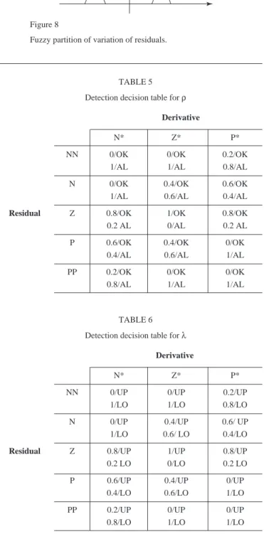
Three fuzzy sets (N*, Z* and P*) are used to describe the variation of residual (Fig. 8).
The fuzzy sets form 15 combinations (Tables 5 and 6). The linguistic label OK means that the situation is normal and AL that the situation is abnormal (alarm). Symbolic fuzzy sets are used to express the meaning of these labels.
µ/label expresses a membership of value µto the label. Obviously AL and OK are complementary. For instance, if the residual is positive medium with a negative variation, this means that it is decreasing, so the situation is not so bad (0.6/OK). On the other hand, for positive variations, the situation is bad and worsening (1.0/AL). A similar table is based on λ(t) in order to isolate the faults, with a symbolic reasoning concluding that the fault is local to a variable (LO) or upstream (UP) in the graph. For instance, if the residual
λ(t) is medium positive with a positive variation, this means that it is increasing, there is a local fault that is increasing (0.8/LO) and (0.2/UP).
Fuzzy reasoning provides three membership functions between 0 and 1. The first function informs about the state of the variable, OK/AL. The gradual evolution between 0 and 1 characterises the evolution of the variable from a normal state to an undesirable one (detection). This transition is used in the supervision interface representing the causal graph for the operators—in terms of a colour code. The value that characterises the state of the variable is used to colour the contour of the nodes. The contour of the node is red when a fault is surely detected (µ/AL = 1) and green when not (µ/OK = 1). In between, it evolves through yellow, orange, etc.
The average value of the two other membership functions informing on the localisation of the fault (LO/UP) is used to colour the arcs of the graph. The input arrows are green for a surely local fault and red for a surely upstream one.
The use of transition colours shows that fuzzy logic is useful to follow the variable gradual evolutions. Moreover this approach is close to human thinking and is well adapted to real processes with model uncertainties and measurement imprecision.
TABLE 5 Detection decision table for ρ
Derivative
N* Z* P*
NN 0/OK 0/OK 0.2/OK
1/AL 1/AL 0.8/AL
N 0/OK 0.4/OK 0.6/OK
1/AL 0.6/AL 0.4/AL
Residual Z 0.8/OK 1/OK 0.8/OK
0.2 AL 0/AL 0.2 AL
P 0.6/OK 0.4/OK 0/OK
0.4/AL 0.6/AL 1/AL
PP 0.2/OK 0/OK 0/OK
0.8/AL 1/AL 1/AL
TABLE 6 Detection decision table for λ
Derivative
N* Z* P*
NN 0/UP 0/UP 0.2/UP
1/LO 1/LO 0.8/LO
N 0/UP 0.4/UP 0.6/ UP
1/LO 0.6/ LO 0.4/LO
Residual Z 0.8/UP 1/UP 0.8/UP
0.2 LO 0/LO 0.2 LO
P 0.6/UP 0.4/UP 0/UP
0.4/LO 0.6/LO 1/LO
PP 0.2/UP 0/UP 0/UP
0.8/LO 1/LO 1/LO
2.1.4 Application to the FCC Pilot Plant
In the FCC application, the model that is used contains 29 components, 40 variables and 25 causal relations. It was derived from a larger model containing 323 variables and 282 causal relations following the methodology presented in Section 1.
Figure 7
Fuzzy partition of residuals.
Figure 8
Fuzzy partition of variation of residuals.
N Z Z P PP
The causal graph can be displayed on the operator interface and used as a visual tool for fault detection and isolation on variables as well as for explanation. A node is green when no discrepancy is detected (for example, pc30 in Figure 9) and red when a discrepancy is detected (for example pt20), arcs influencing a variable are red for a local fault (for example between pt20 and pc20) and green otherwise (for example between pc30 and pt30) (cf. Figure 9 where red arcs appear in bold and red nodes in grey circles).
Figure 9 presents the causal graph which is used for development purposes. Figure 10 presents the alarms and synoptic which are given to operators.
Figure 9
Example of the causal graph used in development.
Figure 10
Visualisation of alarms in the FCC synoptic.
2.2 Fault Isolation on Physical Components
Having detected a discrepancy between predictions and observations, the aim of the isolation process is to search for the original possible cause(s) and to elaborate of a list of potential diagnoses. A diagnosis is a minimal set of components for which the invalidation of the normal behaviour assumptions yields (SD, COMP, OBS) consistent, where:
– SD is a formal description of the system including assumptions of normal behaviour for the set COMP; – COMP: set of components;
– OBS: set of observations.
In the proposed approach, the causal graph acts as the SD and the influences attached to the edges are the elements of COMP.
The diagnostic process is initiated as soon as a variable is isolated as being the source of the detected misbehaviour (deduced from the local residual). For this variable (i.e. a node in the causal graph), conflict generation procedure traces the causal graph, following the intuition that the influences which may be at the origin of the misbehaviour of variable X are those related to the edges entering into X (and only those ones).
The diagnostic generation is based on generating the minimal hitting sets of the collection of conflicts generated by the above algorithm (Cordier et al., 2000) (a set S that has a non-empty intersection with every set in a collection of sets C is called a hitting set of C; if no element can be removed from S without violating the hitting set property, S is considered to be minimal). A diagnosis is hence a set of components such that its intersection with each conflict set is not empty.
Different hypotheses referring to exoneration assump-tions may be considered (Travé-Massuyès et al., 2001). Exoneration implies that a fault always manifests itself, which depends on the existence or absence of compensatory effects within the system as well as on the sensitivity of the fault detector. In the FCC application, practical con-siderations led us to assess that the exoneration assumption is valid for sensors. We assess that sensors are reliable components, i.e. the sensors associated with the arcs directly influencing a non-misbehaving variable are considered to be normal.
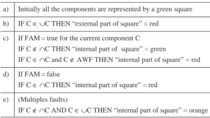
Figure 11 is an example of a list of components of the FCC pilot plant associated to a colour code. The following abbreviations are used:
– C: component; – ∪C: union of conflicts; – ∩C: intersection of conflicts; – FAM: fault always manifested; – AWF: arc without faults.
Figure 11
Visualisation of faulty and non-faulty components.
TABLE 7
Colour code displayed in the squares in Figure 11 a) Initially all the components are represented by a green square b) IF C ∈ ∪C THEN “external part of square” = red
c) If FAM = true for the current component C IF C ∉ ∩C THEN “internal part of square” = green
IF C ∈ ∩C and C ∉AWF THEN “internal part of square” = red d) If FAM = false
IF C ∈ ∩C THEN “internal part of square” = red e) (Multiples faults)
IF C∉ ∩C AND C ∈ ∪C THEN “internal part of square” = orange
The square colour ranges from red for incriminated single fault components to green for non incriminated components, and can be orange when the component can take part in a multiple fault.
2.3 Fault Identification
Having estimated the list of physical components which have an abnormal behaviour, the aim of fault identification is to generate a message in natural language describing the particular fault on a suspected component to the operator.
To complete this task, each physical component is associated with semi quantitative models of its abnormal behaviour. These models (Heim et al., 2001), obtained from human operator knowledge (Hazop analysis), take the form of AND/OR fault/symptom tree (cf. Fig. 12). They are activated only when the component is suspected to have an abnormal behaviour.
Symptoms take the form of signal analysis: increases , decreases , pulse and , oscillation , steps and .
When there exists negligible and complicated phenomena that are not modelled with the causal model, the abnormal behaviour model allows refining the diagnosis concerning
those phenomena. It gives also a list of actions in order to verify and to counteract the fault.
Figure 13 is an example of an expert graph obtained for the stripper. It indicates that if the pressure stripper is low and the valve opening that regulates the pressure is 0%, then there is a leakage between the riser and stripper. In order to confirm this diagnosis, the operator has to verify that the pressure set-point is different from the measure. The repercussions are then defined. They depend on the type of regulation used (cascade 1 or 2).
Figure 12
Semi-quantitative abnormal model structure.
Figure 13 Riser expert graph.
3 IMPLEMENTATION
This approach was implemented using Gensym’s G2 soft-ware. G2 allows object oriented and graphical programming of real time application. Causal graph nodes and directed arcs are represented by objects. Causal graph can easily be modified adding a node and connecting it with other nodes. Selecting any arc enables to change its transfer function parameters, and to modify its associated components list. In the fault/symptom tree associated to each physical component, symptoms and messages delivered to the operator are represented by objects. Relationships between symptoms and faults are symbolised by directed arcs. Parameters can be changed (variable identity, amplitude, frequency, etc.) to change the sensitivity of the signal analysis. This allows to tune an application and to apply it to different processes or sites.
Symptom 1 Logical operations Fault identification Symptom n •••
4 FCC APPLICATION 4.1 FCC Process
FCC process includes many subsystems (two regenerators, a reactor, a separation column, pipes, valves, etc.). The reactor riser temperature is very close to the metallurgical limits for optimum production. As a result of cracking, carbonaceous products (called coke) get deposited on the catalyst, which decreases the effectiveness and the lifetime of the expensive catalyst. This one is continuously regenerated in the regenerator by blowing in air. Coke is combusted to CO, CO2, and H2O. The amount of CO vented out through the stack gas is very crucial from an environment point of view, and one of the challenges for our application is not to violate the environmental threshold and to achieve an optimum performance in the face of disturbances. There is a constant flow of regenerated and spent catalyst between the reactor and the regenerator. This flow is partly driven by the pressure differential between the reactor and regenerator, and the remaining momentum is supplied by the lift air blower. The fractionator’s section separates the product hydrocarbons for further processing. A feed system consisting of low-level flow controllers and a preheating furnace pre-processes the feed for cracking.
The FCC chosen is a pilot plant. Table 8 describes order of magnitudes of the physical variables in a real FCC and in a FCC pilot plant.
TABLE 8
Differences between an industrial FCC and the FCC pilot plant
Characteristics Industrial FCC pilot
FCC plant Capacity 40 000 bbl/d 2 bbl/d Regenerator long 15 m 1 m Regenerator diameter 8 m 20 cm Riser long 35 m 7 m Riser diameter 1 m 2 cm Feed flow 245 t/h 6 kg/h Catalyst flow 1500 t/h 40 kg/h
Total mass of catalyst 300 t 40 kg
Contact time in the riser 2 à 4 s 1 s
Contact time in the stripper 1 min 15 min Contact time in each regenerator riser 5 min 20 min
In the FCC pilot plant (Fig. 14), the catalyst circulates in a physical closed loop: it goes from the stripper (R3), to the 1st regenerator (R1) then to the 2nd regenerator (R2) then to the riser (R1) and finally comes back to the stripper (R3). Catalyst circulation is ensured by pipes: the lift (T2), the stand pipe (T3) and the riser (T1). Riser is also a reaction zone. The feed is put in contact (via V6) with the catalyst in the riser during few seconds and immediately catalyst and
Figure 14
FCC pilot plant process variables.
reaction products fall in the stripper. The stripper R3 separates valuable components and low boiling point molecules from the catalyst and the coke. Coke is a reaction secondary product composed of high boiling point molecules. Valuable components are separated from low boiling point molecules by a separation column (C1). A filter (F1) between the column and the stripper prevents catalyst from going in the separation column. The catalyst and the coke are driven to the first regenerator R1 through a valve V4. Coke is partially burnt in the first regenerator. The second regenerator R2 finishes this combustion. At the output of the second regenerator, the hot regenerated catalyst that is driven to the bottom of the riser rapidly reacts with the feed. Three pressure control valves V1, V2, V3 are used to control respectively the stripper, 1st regenerator and 2nd regenerator pressures. Nitrogen flows are controlled to ensure the catalyst circulation (V7 to V12). Air flows are controlled to ensure the coke combustion (V13 and V14). Catalyst levels in stripper and separation column are controlled respectively by valves V4 and V5. Filters F2 and F3 respectively prevent catalyst from going into V2 and V3.
Problems that occur in a industrial FCC are (Sadeghbeigi, 2000):
– catalyst circulation; – catalyst loss; – coking/fouling; – flow reversal;
– high regenerator temperature; – afterburn;
– hydrogen blistering; – hot gas expander;
– products quality and quantity.
Problems that occur on the FCC pilot process have been classified in 6 types:
– blockage (pipe, valve, etc., cf. scenario 1); – leakage; DPDR FNL FR1 PR1 LR1 FNR1 FNS LS PS DPS PC FS FNR DPR DPC FFR FOR1 DPR1 LR2 PR2 DPR2 FNR2 FOR2 FNST DPST DPL F3 V3 R2 V10 V2 C1 V1 V5 T1 V6 V7 F1 V13 V9 V8 R3 R1 V4 V12 V14 V11 T3 T2
– change in the material properties (catalyst, etc.); – bad operation (operator, etc., cf. scenario 2); – sensor faults (cf. scenario 3);
– utilities (gas, electricity, etc., cf. scenario 4). 4.2 Scenarios Description
This paragraph presents scenarios that happened on the FCC pilot plant.
In the application, the assumption is made that a sensor fault always manifests (Section 2.2). Therefore, in the following sections, sensors are exonerable components.
Table 9 presents the detection time obtained using the presented method, named ASCO, with the one an operator would obtain (ASCO stands fo: Aide à la Supervision et à la Conduite pour les Opérateurs). Theses times are suggestive, and are obtained from historical data.
– column 1 describes the type of fault; – column 2 describes the failure;
– column 3 gives the detection time for ASCO; – column 4 gives the detection time for an operator.
The following sections present four scenarios of abnormal situation.
4.2.1 Scenario 1
This scenario corresponds to a blockage between stripper (R3) and separation column (C1). Catalyst is carried in this line by gas flow from stripper (R3) toward the separation column (C1). Figure 15 shows influences provided by the causal graph in this scenario (without sensors). For example, RV3 component (controller of valve V3) is in the support (list of physical components) of influences SPS->OPPS and OPPS->PS.
Figure 15
Influences and their underlying components.
Faults are detected on variables PS (R3 pressure), OPPS (V1 opening value), DPR (Riser pressure drop), DPL (lift pressure drop), DPS (cocker pressure drop), FS (V1 effluent flow), LR2 (second regenerator level), LR1 (first regenerator level), PC (Separation column sky pressure), DPC (V4 pressure drop) and OPLS (V4 opening value). These variables are grey in Figure 16.
Faults are isolated on variables FS (V1 effluent flow) and PS (R3 pressure). Arcs influencing these variables appear in bold in Figure 16.
Figure 17 presents global and local residuals of stripper (R3) pressure: rPS(t) (left), λPS(t) (right). Figure 18 presents global and local residuals of V4 pressure drop: rDPC(t) (left) and λDPC(t) (right). Thresholds aPSand aDPCare symbolised by horizontal lines.
∆ ∆
SPS->OPPSPS->OPPSOPPS->PSOPPS->F
TABLE 9
Time detection in practical scenarios
Faults Description Time for detection
ASCO Operator
Blockage 1. Blockage of pipes between stripper and column 5 min 50 min
2. Blockage of valve on the first regenerator 5 min 15 min
8. Gas bubbles in the pump circuit 20 min 1 h
5. Filters in the first regenerator 1 min 15 min
6. Filters in the second regenerator blocked 1 min 15 min
Sensor faults 3. Abnormal level in the first regenerator 1 min 20 min
Operator faults 4. Bad operator actions creating disturbances in the process 1 min 5 min
8. Gas bubbles in the pump circuit 1 min 10 min
11. Gas present between the first and second regenerator 5 min 10 min Utilities 7. Lack of air to operates the regulation valves in two regenerators 5 min Not detected
Process 9. Stand pipe drain 1 min 10 min
10. Catalyst present between the striper and the separation-column 55 min 1 h Wear 12. Abnormal behaviour of level regulation valve in the stripper 55 min 20 min
SFNS SFFR SFNR SFNL SFOR2 SFNR2 SFNR1 SFOR1
OPFNS
SPS OPFFR OPFNL OPFOR2 OPFNR2 OPFNR1 OPFOR1
FNR2 FNR1 FOR2 FNL FFR FS LR2 DPS FR2 FR1 DPR2 DPL DPR1 PC FNS FNST DPST DPDR DPR DPSC SPR2 OPFNR FNR FOR1 SPR1 OPR2 PR1 OPR1 DPC SLS OPLS LS LR1 PR2 OPPS PS Figure 16
Causal graph in scenario 1.
T1 T2
Figure 17
rPS(t), λPS(t) (variation of local and global residuals of PS).
T3
Figure 18
A fault is detected on PS (R3 pressure) because rPS(t) is greater than aPSfor t > T1. This fault is local because λPS(t) is greater than aPSfor t > T2. A fault is detected on DPC (V4 pressure drop) because rDPC(t) is greater than aDPCfor t > T3. But this fault is upstream because λPS(t) is always inferior to aDPC.
The set of components associated with the arcs influencing FS (V1 effluent flow) defines a conflict because
λ(FS)> 0. This conflict is {C1, F1, V1, V5, FSt, OPPSt, PSt} where the notation Ytrefers to the component that transmits the value of Y. The set of components associated with the arcs influencing PS (R3 pressure) defines a conflict because
λ(PS)> 0. This conflict is {C1, F1, R3, T1, V1, V5, OPPSt, FNSt, FFRt, FNRt, PSt}.
Knowing these two conflicts, minimal diagnoses are {C1}, {F1}, {V1}, {V5}, {OPPSt}, {PSt}, {FSt, R3}, {FSt, T1}, {FSt, FNSt}, {FSt, FFRt}, and {FSt, FNRt} (simple and multiple faults without exoneration). Theses sets of components intersect both conflicts. If we consider only simple faults, following diagnoses are obtained: {C1}, {F1}, {V1}, {V5}, {OPPSt}, {PSt}.
Sensors are considered as exonerable components. Therefore when the local residual of a variable is lower than its threshold, sensors measuring upstream variables are removed from diagnoses. In this scenario, the local residual of LR2 (second regenerator level) is lower than aLR2. Consequently, sensor PStthat is associated with this residual is removed from diagnoses.
Sensor OPPSt (V1 opening value) is also considered not faulty because its local residual is also lower than aOPPS. Therefore, sensor minimal diagnosis is Ø, thus, no single sensor fault is suspected.
Following diagnoses are then obtained: {F1}, {C1}, {V1},{V5}. Fault/symptom tree of F1, C1, V1 and V5 are activated. The signal analysis generates two symptoms: PS (R3 pressure) , OPPS (V1 opening value) . A qualitative expert rule (cf. Fig. 19) is launched and the following message is delivered to the operator: “Fault: Blockage of
Figure 19
Expert graph activated for scenario 1.
V1 or C1. Confirmation: By pass C1. If pressure PS (R3 pressure) decreases then C1 abnormal else V1 abnormal.”
V1, F1, C1 and V5 fault/symptom trees are made of several other rules but no other combination of symptoms is observed . Therefore, no other conclusion can be considered. Without any diagnostic module, operators may not detect the fault before security systems automatically halt the process, after 40 min. With the diagnostic module, the fault is isolated 5 min after its inception, allowing 35 min for operators to act on the process.
V1 is composed of two parallel valves V1a and V1b. If only one valve (V1a for instance) is blocked then operation can be maintained controlling PS (R3 pressure) only with V1b. The operator has time to change V1a.
4.2.2 Scenario 2
This scenario corresponds to the formation of bubble of gas in the feeding pump because the valve V6 temperature, TV6, is too high. The variables directly affected are FFR (V6 feed flow) and OPFFR (V6 opening value). Faults are detected on {OPFFR, FFR, PS, OPPS, FS, DPS, PC, DPR, DPL, LR2, LR1}. Faults are isolated on {FFR,OPFFR}. Components associated with the arcs influencing FFR (V6 feed flow) define a conflict. This conflict is {V6, RV6, FNT, OPFFRt, FFRt}. Components associated with the arcs influencing OPFFR (V6 opening value) define a conflict. This conflict is {V6, RV6, FNT, OPFFRt}. Minimal diagnoses are {V6}, {RV6}, {FNT} and {OPFFR}.
The operator is informed that sensor OPFFRtis suspected to be faulty. In fact this sensor is not faulty. Having more knowledge on sensors will enable to exonerate this sensor. Fault symptom trees of V6, RV6 and FNT are activated. The qualitative model associated with SC2 fault is given by:
[(F1 ) or (F1 )] and [TV6>]
(F1 ) and TV6>are observed making signal analysis. The qualitative rule (F1 ) and (TV6>) is observed therefore this message is delivered:
Temperature TV6is a variable that has not been introduced in the model but that is interpreted in the fault identification module.
In this scenario, the only delivered message is Message 2. The time of abnormal behaviour occurrence is 50 minutes. 10 minutes are necessary to the operator to isolate the fault without the diagnostic module. The diagnostic module instantaneously generates the message.
The operator has to stop feeding and to wait until TV6 decreases. Feed can then be reactivated. If the operator does not react rapidly enough the FCC pilot can go into a
Message 2: “Gas bubbles in the feeding pump V6. Stop feeding and wait until TV6decreases”.
PR3 OPV3 OPV3 OR Message AND AND PR3 > >
not permitted state that activates automatically security monitoring functions.
4.2.3 Scenario 3
This scenario corresponds to a fault on sensor LR1 (first regenerator level). The variable which is directly affected is LR1. A fault is detected and isolated on LR1. Components associated with the arcs influencing LR1 are {T1, T2, T3, T4, R1, R2, R3, V4, LR1t, LR2t, LSt}. Therefore, conflicts are {T1}, {T2}, {T3}, {T4}, {R1}, {R2}, {R3}, {V4}, {LR1t}, {LR2t} and {LSt}.
Sensor LR2t (second regenerator level) is not faulty because λ(LR2) = 0. Sensor LSt is not faulty because
λ(LS) = 0. The operator is informed that sensor LR1t(first regenerator level) is suspected.
Fault symptom tree of T1, T2, T3, T4, R1, R2, R3 and V4 are activated. The identification module does not deliver any message because the FCC behaves normally.
The time of abnormal behaviour occurrence is approxi-mately 40 min. 5 min are necessary for the operator to isolate the fault without the diagnostic module. Fault isolation is instantaneous with the diagnostic module. LR1 sensor (first regenerator level) is blocked with catalyst. The operator has to create a gas stream inside the sensor to repair it.
4.2.4 Scenario 4
This scenario corresponds to a decrease of the air network pressure. The variables directly affected are OPFOR1 and OPFOR2. This network pressure is not transmitted to the diagnostic module. Faults are compensated by control loops (RV13 and RV14) and do not propagate in the causal graph. Faults are detected and isolated on OPFOR1 and OPFOR2.
Conflicts are {RV13, V13, ONT, OPFOR1t} because
λ(OPFOR1)>0 and {RV14, V14, ONT, OPFOR2t} because
λ(OPFOR2)>0. A minimal diagnosis is {ONT}, so, ONT fault symptom tree is activated. Symptoms (OPPR1<) and (OPPR2<) are observed. Therefore, the following message is delivered to the operator: “Decrease of the air pressure network. Check if this measure is low”. Symptom/trees associated to other diagnosis do not provide any other conclusion.
The qualitative model associated with SC4 fault is: [(OPPR1 ) or (OPPR1<)] or [(OPPR2 ) and (OPPR2<)]
(OPPR1<) and (OPPR2<) are observed, therefore, the following message is therefore delivered to the operator:
In this scenario, the only delivered message is Message 4. The time of abnormal behaviour occurrence is approxi-mately 15 min. This fault was not detected by the operator
because the gas flows were maintained at their set point. The diagnostic module generates the message 3 min after the fault occurrence. Thanks to this information, the operator can engage actions on the air pressure network before its pressure is too low.
CONCLUSION
This paper presents a methodology to apply a diagnostic method to an industrial size process. The combination of complementary techniques (modelling, fault detection, fault isolation and fault identification) is used.
Modelling is carried out using a causal model which describes the normal influences among process variables and supports qualitative and quantitative information. The initial knowledge consists in the process variables (endogenous and exogenous variables), and the set of formal relations, related to physical components, that describe the variables. This knowledge constitutes the structural relation model. The application of a causal ordering algorithm to the structural relation model provides the causal graph, which exhibits the causality underlying the set of relations in the form of a set of directed influences between variables. Other operations are further necessary, due to the practical difficulty in quantifying the relations involved in the causal graph with theoretical knowledge. Model identification and parameter estimation is generally used, which is only possible if data are available for the variables. A reduction operation consists in eliminating unknown variables from the graph. An approximation operation results in an approximated causal model that contains only known process variables connected by quantified relations. At this step the model is ready for causal simulation which is to say for computing the endogenous variables from the measured values of the exogenous ones. As the influences are associated to specific physical components, the approximated causal model is also suitable for supporting diagnosis, i.e. fault isolation.
Fault detection is carried out using classical analytical redundancy. The quantitative causal model provides refer-ences characterising the normal behaviour of the process. Comparing measures with these references, the fault detection module determines whether measured variables have an abnormal behaviour or not, and generates alarms. For each variable, the fault detection module generates two references considering a local environment and a global one (given by process set points and measured external disturbances). This is important for detection of incipient faults and for safety which absolutely requires checking critical variables in regards to their set points.
Isolation is carried out applying a hitting set algorithm on the list of components associated to edges connected to variables which have an abnormal behaviour. This allows Message 4: “Decrease the air pressure network.