HAL Id: hal-01333600
https://hal.archives-ouvertes.fr/hal-01333600
Submitted on 15 Sep 2016
HAL is a multi-disciplinary open access
archive for the deposit and dissemination of
sci-entific research documents, whether they are
pub-lished or not. The documents may come from
teaching and research institutions in France or
abroad, or from public or private research centers.
L’archive ouverte pluridisciplinaire HAL, est
destinée au dépôt et à la diffusion de documents
scientifiques de niveau recherche, publiés ou non,
émanant des établissements d’enseignement et de
recherche français ou étrangers, des laboratoires
publics ou privés.
Records
Martin Bodin, Thomas Jensen, Alan Schmitt
To cite this version:
Martin Bodin, Thomas Jensen, Alan Schmitt. An Abstract Separation Logic for Interlinked Extensible
Records. Vingt-septièmes Journées Francophones des Langages Applicatifs (JFLA 2016), Jan 2016,
Saint-Malo, France. �hal-01333600�
for Interlinked Extensible Records
Martin Bodin, Thomas Jensen & Alan Schmitt
Inria, FranceRésumé
The memory manipulated by JavaScript programs can be seen as a heap of extensible records storing values and pointers. We define a separation logic for describing such structures. In order to scale up to full-fledged languages such as JavaScript, this logic must be integrated with existing abstract domains from abstract interpretation. However, the frame rule—which is a central notion in separation logic—does not easily mix with abstract interpretation. We present a domain of heaps of interlinked extensible records based on both separation logic and abstract interpretation. The domain features spatial conjunction and uses summary nodes from shape analyses. We show how this domain can accommodate an abstract interpretation including a frame rule.
1.
Introduction
The memory of a JavaScript program is a dynamic and complex heap of extensible records storing values and pointers. Fields can be added and removed from records dynamically, and their presence can be tested. Moreover, records are not constrained by a static type structure, which further complicates the analysis of the shapes that these interlinked objects may form. Obtaining a good approximation of the memory structure of a JavaScript program is a challenge for static analysis, even if we restrict other features of the language such as computed field names and dynamic code generation.
In this paper, we present a solution to this challenge, by mixing elements of separation logic and shape analysis, and integrating them into an abstract interpretation framework. Separation logic in itself is not adequate for describing the inter-connected heaps of JavaScript. First, separation logic is based on some additional structures, such as lists or trees. For JavaScript, such structures can be difficult to identify, as illustrated by Gardner et al. [?]. Second, JavaScript native structures tend to not separate nicely. Gardner et al. propose to remedy this through a partial separation operator ⊔⋆ (“seppish”). The formula 𝑃 ⊔⋆ 𝑄 describes a heap which can be split in two heaps, one satisfying 𝑃 and the other 𝑄; but these two heaps do not need to be disjoint. Here, we pursue this idea, but instead of introducing a new operator in separation logic, we inject ideas from shape analyses, and use summary nodes for modelling the portion of memory that may be shared. In this way, we move the approximation into the shape structures while keeping a precise separation operator ⋆.
The work described here is part of a larger project on certified static analyses in which static analysis tools are developed an proved correct based on a mechanised formalisation of the semantics of the underlying language. More precisely, the aim is to build on the JSCert [?] semantics for JavaScript, a pretty-big step operational semantics [?] entirely written in Coq. The size of the JavaScript’s semantics imposes that we take an approach that is both principled and mechanisable. We base the development on the theory of abstract interpretation. Abstract interpretation [?] provides a powerful theory for finding and proving loop invariants within a program, assuming minimal structure on the
This research was partially supported by the French ANR-10-LABX-07-01 Laboratoire d’excellence CominLabs and ANR-14-CE28-0008 project Ajacs.
space of abstract domains. For the mechanisation, certification in proof assistants such as Coq is needed. We have previously built a Coq library [?] providing the building blocks for constructing an abstract interpretation from a pretty-big step operational semantics, following initial ideas of Schmidt [?]. In that paper, we showed how to derive abstract rules from concrete ones in such a way that abstract derivations are correct by construction. Here, we show how to extend this approach with abstractions of heaps using techniques from both separation logic and shape analysis, in order to give reasonable results for JavaScript.
The abstract domains arising from separation logic do not have the rich structure of lattices encountered in many abstract interpretations. The theory of abstract interpretation, however, does generalise to the setting where the underlying structure is that of only a subset of a pre-order. We shall hence use this more general framework, which provides the same correctness guarantees but does not explain how to compute a best analysis result.
Separation logic provides useful notions for the analysis of heap-manipulating programs. In separation logic, abstract rules are only given locally: they only state what is changed by a given program, assuming that everything not mentioned is left unchanged. The frame rule then allows to add an unchanged partial heap to the analysed result. This mechanism is very powerful to locally reason about programs. However JavaScript introduces some new issues about the frame rule: Reynolds [?, Section 3.5] stated that the frame rule can not be applied as-is if the language allows constructions similar to JavaScript’s delete operator. We address this issue using a special value ⊠.
The main contributions of this paper are as follows.
• A combination of separation logic and shape analysis, which allows to use the separation ⋆ for disjoint domains, and shapes for complex domains with potential sharing.
• An alternative to the ⊔⋆ operator that better fits the frame rule.
• An integration of separation logic into an abstract interpretation framework based on pre-orders and big-step operational semantics, extending our previous work [?].
The paper is organised as follows. We first present our toy language OWhile. Our logic is presented in two steps: first, a logic over abstract domains is built in Section ??; its structure should not be surprising to a reader familiar with separation logic. A crucial step of the approach is the addition of membranes, in Section ??, to deal with the frame rule. Second, we add the summary nodes from shape analyses to the domain in Section ??. Section ?? presents how we build our program logic for OWhile, leading in Section ?? to the correctness of our abstract semantics. Section ?? examines related work and Section ?? concludes.
2.
The OWhile Language
We define our analyses on a small imperative language with interlinked records, called OWhile. This language is inspired from JavaScript’s memory model but we shall disregard all aspects related to prototype inheritance or type conversion. We can create new records (which we call objects), and read, write, and delete their fields (also called properties in JavaScript). Records are interlinked because their fields may contain pointers to other objects.
The syntax of our language is presented in Figure ??. A detailed version of the concrete semantics can be found in Appendix ??, but it comes with no surprises for a pretty-big-step semantics [?]. There are only numbers in the language, so for the purpose of branching (instructions if and while), the number 0 behaves as false, and any other number as true. The operation ? non-deterministically returns a number. Fresh objects are created by the {} expression. We can access the field f of an object computed by 𝑒 through 𝑒.f. We can check the presence or absence of a given field f in an
𝑠 ∶∶= skip | 𝑠1; 𝑠2 | if 𝑒 𝑠1𝑠2 | while 𝑒 𝑠 | throw |x∶= 𝑒 | 𝑒1.f∶= 𝑒2 | delete 𝑒.f (a) Statements 𝑒 ∶∶= 𝑛 ∈ ℤ | ? |x∈ Var | nil | {} | 𝑒.f |f in𝑒 | ¬ 𝑒 | = 𝑒1 𝑒2 |1 𝑒1 𝑒2 (1 ∈ {>, +, −}) (b) Expressions
Figure 1: The syntax of the OWhile language
object computed by 𝑒 through f in𝑒, which returns 1 if the field is present and 0 otherwise. As in JavaScript, writing to the fieldfof an object adds the field if it is not already present, and deleting an object’s field succeeds even if the field is absent. There is no explicit declaration of variables: as for fields, writing a variable which is not defined creates it. A program may abort for the following reasons: explicitly running throw, reading a variable or a field that is not assigned, or accessing the field of a value that is not an object. The state 𝑆 of a program is composed of two components.
• An environment (also called store in JavaScript parlance) 𝐸 ∶ Var ⇀ Val, where Var is the set of variable names and Val is the set of values. A value 𝑣 ∈ Val can either be a location 𝑙𝑖
(including the special null location 𝑙0, always out of the domain of 𝑆), or a basic value 𝑛 ∈ ℤ.
• A heap 𝐻 ∶ Loc ⇀ 𝔉 ⇀ Val, where Loc = {𝑙𝑖∣ 𝑖 ∈ ℕ⋆} is the set of non-null locations, and 𝔉 the
set of field names. We assume 𝔉 to be infinite.
We define dom (𝑆) to be dom (𝐸) ∪ dom (𝐻) where 𝐸 and 𝐻 are the respective environment and heap of 𝑆. The function fresh takes a state 𝑆 and returns a location fresh in 𝑆, i.e., 𝑙𝑗∉ dom (𝐻).
3.
Abstract Domains
3.1. Abstract State Formulae
In this section we build a separation logic over an abstract domain of base values. There are various ways of representing separation logic; our logic is based on the work of [?]. Abstract state formulae 𝜙 ∈ State♯ model pairs of concrete heaps and stores. These formulae are defined as follows.
𝜙 ∶∶= emp | 𝜙1⋆ 𝜙2 |x= 𝑣̇ ♯ | 𝑙 ↦ {𝑜} 𝑜 ∶∶=f∶ 𝑣♯, 𝑜 | _ ∶ 𝑣♯
These formulae make use of abstract locations 𝑙 ∈ LLoc♯. These locations are identifiers which
are meant to represent one concrete (non-null) location. In the concretisation of formulae, abstract locations are related to concrete locations by a valuation 𝜌 ∶ LLoc♯ ⇀inj Loc (where ⇀inj denotes a partial injection). Concrete locations in Loc are written with an exponent 𝑙𝑖whilst abstract locations
use indexes or primes: 𝑙, 𝑙𝑖, or 𝑙′.
The structure of the abstract domain for values 𝑣♯∈ Val♯ is described in detail in Section ??. For
now, we just note that this abstract domain contains abstract locations (detailed below) and abstract properties of numeric values (sign, parity, intervals, …). The concretisation function 𝛾𝜌 of abstract
values relates them to sets of concrete values.
The formula emp describes the empty heap and empty environment. The spatial conjunction 𝜙1⋆𝜙2
describes the set of all heaps and environments which we can separate into two smaller heaps and environments, each respecting one of the two sub-formulae 𝜙1and 𝜙2. The ⋆ operator is commutative,
xsatisfies the property 𝑣♯. We follow the tracks of [?] and do not consider this formula pure. As we
are not interested in concurrency in this paper, we use a simpler version than [?] where we either have full permission over x ifx = 𝑣̇ ♯ is present, and no permission otherwise. The construction 𝑙 ↦ {𝑜}
describes the set of heaps whose only defined location 𝜌 (𝑙) points to an object abstracted by {𝑜}. Objects are abstracted as a list associating fields to abstract values, with an additional default abstract value for the other fields present in the object.1 All the specified field names of an object
are supposed to be different. An abstract object {f1∶ 𝑣♯1, … ,f𝑛∶ 𝑣 ♯
𝑛, _ ∶ 𝑣♯𝑟} represents the set
of objects whose respective fields f1, …, f𝑛 are abstracted by respectively 𝑣 ♯ 1, …, 𝑣
♯
𝑛, and all the
other fields are abstracted by 𝑣♯𝑟. Abstract values also include the possibility to state that a field is
undefined. This is expressed through the special value ⊠. The abstract object {f∶ ⊠,g∶ 𝑣♯, _ ∶ ⊤}
thus describes the set of objects such that each object has no fieldfand its fieldgcan be abstracted by 𝑣♯. Similarly, {_ ∶ ⊠} describes the singleton of the empty object, which is returned by {}.
An alternative approach to model heaps and objects is to allow the separation of fields themselves, as in 𝑙7−→f 𝑣♯1⋆ 𝑙7−→g 𝑣♯2, in a way similar to [?]. We experimented with this approach and discovered that it results in complex interactions with the frame rule. We thus follow a simpler approach here.
3.2. Abstract Values and Abstract Object
Our separation logic formulae are parameterized over an abstract domain describing the base values which variables and fields can contain. In line with the dynamic typing of JavaScript, we shall consider an abstract domain containing both numerical values and locations. Hence, a variable may contain both types of values depending on the flow of control, and the abstract domain has to be able to join such values together.
In addition, when analyzing JavaScript’s heap, we must take into account expressions likef in𝑒 whose result depends on the absence of a field. We thus have to track whether fields can be undefined.2
To this mean, we attach a boolean to the abstract values to indicate whether the concrete value can be undefined, as illustrated before with the value ⊠. We use this boolean at two different places: to indicate that a field is possibly undefined, but also to indicate that a variable is possibly undefined.
Suppose a lattice domain ℤ♯carrying abstract properties of numeric, or basic, values (sign, parity,
intervals, …). Such a domain must store information about the different instances of values: basic values, locations, the possibility of being the special location 𝑙0, and the possibility of being undefined.
We define abstract values to be tuples of the form (𝑛♯, nil?, 𝐿, 𝑑), where 𝑛♯∈ ℤ♯ denotes the possible
basic values which can be represented by this abstract value; nil? is a boolean stating whether the value can be 𝑙0(denoted by nil) or not (denoted by nil); 𝐿 ∈ 𝒫
𝑓(LLoc♯) ⊤
denotes the possible location values (𝒫𝑓(LLoc♯)
⊤
denotes the set of finite subsets of LLoc♯ augmented with a ⊤ element); and the boolean 𝑑 ∈ {⊠,□} denotes whether the value can be undefined (denoted by ⊠) or can not (denoted by□). Each part of these tuples carries the information about a kind of value.
For the sake of readability, we will identify the projections of an abstract value 𝑣♯ with 𝑣♯ itself if
all the other projections are bottoms elements of their respective lattice. For instance we will write 𝑛♯
to mean (𝑛♯, nil, ∅,□), nil to mean (⊥, nil, ∅, □), and ⊠ to mean (⊥, nil, ∅, ⊠). We will also identify 𝑙
with (⊥, nil, {𝑙} ,□). To avoid the cumbersome tuple notation, we will use the natural join operation on this domain and write values such as 𝑙 ⊔ ⊠.
The order on the tuple is the usual product order: a tuple is less than another if all its projections are less than the others. Sets of locations are ordered using the usual set lattice. The definition part
1This default field is sometimes called a summary node in the literature; we do not use this name as summary nodes
denote a different concept in this paper.
𝑑 is ordered by □ ⊑ ⊠ as □ forces the value to be defined while ⊠ allows (without forcing) it to be undefined. We similarly define nil ⊑ nil. We use the symbol ⊑ to denote the order within a lattice, that is over abstract values and abstract objects.
We can now define an order on abstract objects as follows: two objects are ordered, {𝑜1} ⊑ {𝑜2} if all the fields of {𝑜1} are associated with a value which is smaller than the value of the same field in {𝑜2}. To check the order relation between two objects, we rely on the default value for all fields not
explicitly mentioned in the object. With this value, we can rewrite the two objects so that they refer to the same fields, using the following rewriting equality,
{f1∶ 𝑣♯1, … ,f𝑛∶ 𝑣 ♯ 𝑛, _ ∶ 𝑣♯𝑟} = {f1∶ 𝑣 ♯ 1, … ,f𝑛∶ 𝑣 ♯ 𝑛,g∶ 𝑣♯𝑟, _ ∶ 𝑣𝑟♯}
which holds provided that g is not one of the f1, …, f𝑛. This order equips abstract objects with a lattice structure, with ⊔ and ⊓ computing the abstract object whose fields are associated to the results of the corresponding operator ⊔ or ⊓ applied on the corresponding fields of the two operands (completed such that they have the same fields):
{f1∶ 𝑣♯1, … ,f𝑛∶ 𝑣 ♯ 𝑛, _ ∶ 𝑣♯𝑟} ⊔ {f1∶ 𝑣′♯1, … , f𝑛∶ 𝑣′♯𝑛, _ ∶ 𝑣′♯𝑟} = {f1∶ 𝑣♯1⊔ 𝑣′♯1, … ,f𝑛∶ 𝑣 ♯ 𝑛⊔ 𝑣′♯𝑛, _ ∶ 𝑣 ♯ 𝑟⊔ 𝑣′♯𝑟}
4.
The Frame Rule
Our main contribution deals with the interaction between formulae and the frame rule. In order to introduce it, we first detail how this rule typically works. The frame rule defines how to extend Hoare
triples using the separation operator ⋆. A Hoare triple 𝜙1, 𝑡 ⇓♯𝜙2 states that the term 𝑡 changes any
heap that satisfies formula 𝜙1 in a heap that satisfies formula 𝜙2. In our setting, a heap satisfies a
formula if it belongs to its concretisation. A heap ℎ belongs to the concretisation of a formula 𝜙1⋆ 𝜙2
if it can be split in disjoint heaps ℎ1 and ℎ2 such that ℎ1satisfies 𝜙1 and ℎ2 satisfies 𝜙2.
Frame
𝜙1, 𝑡 ⇓♯𝜙2
𝜙1⋆ 𝜙𝑐, 𝑡 ⇓♯𝜙 2⋆ 𝜙𝑐
For the frame rule to be correct, it is crucial that if 𝜙1⋆ 𝜙𝑐 is defined (the set of concrete heaps
it denotes is not empty), then 𝜙2⋆ 𝜙𝑐 is defined. In our setting, this may not be the case when new
abstract locations are introduced in 𝜙2. For instance, consider the abstract rule NewObj, which
builds the Hoare triple emp, {} ⇓♯𝑙 ↦ {_ ∶ ⊠}. The result contains an additional location 𝑙 which we
would like to keep fresh from the initial abstract heap emp. However, the frame rule applied as-is can add a new fact about 𝑙 and generate the Hoare triple 𝑙 ↦ {_ ∶ ⊠} , {} ⇓♯𝑙 ↦ {_ ∶ ⊠} ⋆ 𝑙 ↦ {_ ∶ ⊠},
which is wrong as the result formula has an empty concretisation (because 𝑙 is not separated) whilst a concrete derivation tree can easily be derived. This problem also occurs when renaming abstract locations, as is described in Section ??.
To ensure the soundness of the frame rule, we have to introduce scopes for identifiers in a formula. For instance, the scope of a newly created location 𝑙 should be restricted to the result formula, as in emp, {} ⇓♯ (𝜈𝑙 | 𝑙 ↦ {_ ∶ ⊠}): this states that any mention of 𝑙 outside the formula is actually a
different identifier. Since we not only need to restrict the scope of identifiers, but also relate names inside a scope to names outside the scope, we introduce the notion of membrane. A membrane 𝑀 traces the links between these two scopes. Each context added by the frame rule has to be converted when entering a membrane. Membranes behave like substitutions: we can compose them through ∘ and apply them to a formula 𝜙 to update its identifiers. Our version of the frame rule, defined in below, relies on membranes for its soundness.
4.1. Membranes
Membranes 𝑀 are defined as a set of scope changes 𝑚, which can be caused either because a location has been renamed, or because a new location has been allocated. The abstraction Φ of heap and environment is now a couple of a formula 𝜙 and a rewriting membrane 𝑀 , written (𝑀 | 𝜙). We call the simple formulae 𝜙 inner formulae and the membraned formulae Φ formulae.
𝑚 ∈ 𝔐 ∶∶= 𝑙 → 𝑙′ | 𝜈𝑙 Φ ∶∶= (𝑀 | 𝜙) 𝑀 ∈ 𝒫 𝑓(𝔐)
We impose left-hand sides of scope changes to only appear once in a given membrane. We also impose that in a formula Φ = (𝑀 | 𝜙), any location 𝑙 in 𝜙 is present on the right-hand side of a scope change or as a new name 𝜈𝑙 in 𝑀 . We define the domain dom (𝑀 ) of a membrane 𝑀 as the set of left-hand sides of its rewritings, and the codomain codom (𝑀 ) as the union of the set of right-left-hand sides of its rewritings and the set of newly allocated locations. The interface interface (Φ) of a formula Φ = (𝑀 | 𝜙) is the domain of its membrane dom (𝑀 ): these locations are accessible from the outside of the formula. The substitution 𝑀 (𝜙) applied to inner formulae works as expected: it renames every abstract locations either as values or as memory cells. Trivial rewritings such as 𝑙 → 𝑙 are allowed and sometimes required: an abstract location 𝑙 may be unchanged by the membrane, but it still has to be in the interface; the domain names of the inner and scope scopes are independent.
Let us consider a simple example: Φ = (𝑙0→ 𝑙 |x= 𝑙 ⋆ 𝑙 ↦ {̇ f∶ 𝑙, _ ∶ ⊠}). The membrane {𝑙0→ 𝑙}
renames the outer location identifier 𝑙0 to the inner location 𝑙. If the frame rule introduces a context
𝜙𝑐 = 𝑙1 ↦ {f∶ 𝑙0, _ ∶ ⊠} referring to 𝑙0, the integration of 𝜙𝑐 in the membrane leads to the
renaming of 𝑙0 into 𝑙 for a final formula (𝑙0→ 𝑙 |x= 𝑙 ⋆ 𝑙 ↦ {̇ f∶ 𝑙, _ ∶ ⊠} ⋆ 𝑙1↦ {f∶ 𝑙, _ ∶ ⊠}). On
the other hand, if the frame rule introduces a context with a 𝑙 such as 𝜙𝑐 = 𝑙1 ↦ {f∶ 𝑙, _ ∶ ⊠},
this 𝑙 is actually different from the one in Φ. In this case, Φ is 𝛼-renamed, for instance to Φ = (𝑙0→ 𝑙′∣x= 𝑙̇ ′⋆ 𝑙′↦ {f∶ 𝑙′, _ ∶ ⊠}), to avoid the capture of 𝑙 when 𝜙𝑐 enters the membrane.
Note that 𝛼-renaming does not change the interface of a formula: only its codomain is modified. Formulae are used to abstract states (environment and heap), but there are places in our semantics where additional values are carried. In pretty-big-step, we use intermediate terms along the execution, which require to carry additional values. For example, the assignment x ∶= 𝑒 involves two steps (evaluating the expression and updating the state) so we introduce an intermediate termx∶=1whose
semantic context consists of a state and a value to assign tox and whose result is the update state. These values can contain locations and must be placed inside membranes: we shall thus sometimes manipulate formulae of the form (𝑀 ∣ 𝑙 ↦ {𝑜} , 𝑙 ⊔ 𝑙′) where the value 𝑙 ⊔ 𝑙′represents the value of the
intermediate semantic context. All operations defined on usual formulae can be extended to extended formulae. We do not show the details here for space reasons.
4.2.
Separating Formulae
To express the frame rule in our formalism, the frame has to manipulate membranes; we define the operator ..⋆ (read “in frame”) taking two formulae Φ𝑜 = (𝑀𝑜| 𝜙𝑜) and Φ𝑖 = (𝑀𝑖| 𝜙𝑖)—𝑖 stands for “inner” and 𝑜 for “outer”—which intuitively builds (𝑀𝑜| 𝜙𝑜⋆ (𝜙𝑖| 𝑀𝑖)) (this formula does not fit the grammar of formulae as-is): the inner formula is considered in the context of the outer one. This operation is associative, but not commutative. It performs an 𝛼-renaming of the inner identifiers of 𝜙𝑖to prevent conflicts with 𝑀𝑖, then pushes 𝜙𝑜 through the membrane 𝑀𝑖. For instance
for Φ𝑜 = (𝑙0→ 𝑙, 𝑘0→ 𝑘 | 𝑘 ↦ {g∶ 𝑘,h∶ 𝑙, _ ∶ ⊠}) and Φ𝑖 = (𝑙 → 𝑘 | 𝑘 ↦ {f∶ 𝑘 ⊔ nil, _ ∶ ⊠}), the
concrete locations in both formulae. We thus 𝛼-rename 𝑘 into 𝑘′ to avoid name conflict:
(𝑙0→ 𝑙, 𝑘0→ 𝑘 | 𝑘 ↦ {g∶ 𝑘,h∶ 𝑙, _ ∶ ⊠}) ..⋆ (𝑙 → 𝑘 | 𝑘 ↦ {f∶ 𝑘 ⊔ nil, _ ∶ ⊠})
= (𝑙0→ 𝑙, 𝑘0→ 𝑘 | 𝑘 ↦ {g∶ 𝑘,h∶ 𝑙, _ ∶ ⊠}) ..⋆ (𝑙 → 𝑘′∣ 𝑘′↦ {f∶ 𝑘′⊔ nil, _ ∶ ⊠})
= (𝑙0→ 𝑘′, 𝑘0→ 𝑘 ∣ 𝑘 ↦ {g∶ 𝑘,h∶ 𝑘′, _ ∶ ⊠} ⋆ 𝑘′↦ {f∶ 𝑘′⊔ nil, _ ∶ ⊠})
Because of the composition of membranes, 𝑙, which was an identifier introduced by 𝑀𝑜but substituted by 𝑀𝑖, was removed. Membranes are meant to be composed by the ..⋆ operator, and the domain of the inner membrane should thus be in the codomain of the outer one: dom (𝑀𝑖) ⊆ codom (𝑀𝑜).
We define ..⋆ as follows. Given and Φ𝑜 = (𝑀𝑜| 𝜙𝑜) Φ𝑖 = (𝑀𝑖| 𝜙𝑖) such that dom (𝑀𝑖) ⊆
codom (𝑀𝑜), we 𝛼-rename Φ𝑖 into Φ′
𝑖 = (𝑀𝑖′∣ 𝜙′𝑖) such that codom (𝑀𝑖′) ∩ codom (𝑀𝑜) = ∅. We
then make the formula 𝜙𝑜 enter the membrane 𝑀𝑖:
Φ𝑜 ⋆ Φ.. 𝑖= Φ𝑜⋆ Φ.. ′𝑖= (𝑀𝑖′∘ 𝑀𝑜∣ 𝑀𝑖′(𝜙𝑜) ⋆ 𝜙′𝑖)
We are now ready to state our frame rule.
Frame
Φ, 𝑡 ⇓♯Φ′
Φ𝑐⋆ Φ, 𝑡 ⇓.. ♯Φ 𝑐 ⋆ Φ.. ′
Although our program logic is not introduced until Section ??, here is an example of how the frame rule can be used. Consider the program if ? skip (x ∶= ?) where the branch is chosen randomly, one branch does nothing while the other assigns a random value tox. The empty branch of the if can be given the Hoare triple emp, skip ⇓♯emp, and the other branch the Hoare triplex= ⊠,̇ x∶= ? ⇓♯x= ⊤̇
ℤ.
The first branch can then be extended using the frame rule to the triplex= ⊠, skip ⇓̇ ♯x= ⊠. Sincė
both branches now have the same assumption, they may be merged together for the whole conditional:
x= ⊠, if ? skip (̇ x∶= ?) ⇓♯x= ⊠ ⊔ ⊤̇ ℤ.
5.
Adding Summary Nodes
Up to this point, the formulae which we have defined reflect precisely the structure of the concrete heap. However, this approach is not viable in the presence of loops. We need a way to forget about some information of the structure, in particular its size. To this end, we reuse the idea of summary nodes from shape analysis, by adding a new kind of abstract locations 𝑘 ∈ KLoc♯ which represent a
set (finite and possibly empty) of concrete locations. We call them summary locations. As with LLoc♯,
this new set of abstract locations KLoc♯ is supposed to be a new, infinite, set of identifiers. We note
abstract locations as ℎ ∈ KLoc♯⊎ LLoc♯.
Abstract values have been defined in Section ?? as tuples (𝑛♯, nil?, 𝐿, 𝑑), where 𝐿 ∈ 𝒫
𝑓(LLoc♯) ⊤
. We update them to track summary nodes by changing their projection 𝐿 to 𝐿 ∈ 𝒫𝑓(LLoc♯⊎ KLoc♯)
⊤
. Values are thus abstracted by Val♯= ℤ♯× {nil, nil} × 𝒫
𝑓(LLoc♯⊎ KLoc♯) ⊤
× {□, ⊠}.
In formulae, summary locations may occur on the left-hand side of heaps 𝑘 ↦ {𝑜}, denoting heaps where every concrete location in the concretion of 𝑘 maps to a concretion of 𝑜. When 𝑘 occurs as a value, its concretion is any single location denoted by 𝑘. Note the asymmetry in 𝑘 ↦ {f∶ 𝑘, _ ∶ ⊠}, which means that every concrete location represented by 𝑘 has a fieldfpointing to a concrete location in the set represented by 𝑘, but there is no relation between these two concrete locations. In particular, they need not be the same.
. .. 𝑘1.. 𝑘2 {𝑜1} . {𝑜2} ... 𝑘 . {𝑜1} ⊔ {𝑜2} . ⇝
(a) Summarizing two summary nodes
... •.𝑙. {𝑜} . 𝑘 . {𝑜} . ⇝ (b) Summarizing an ab-stract location . . .. 𝑘 .. • . 𝑙 . {𝑜} . f . . . 𝑘 .. • . 𝑙 . {𝑜} . f . ⇝ .. • . 𝑙′ (c) Materialisation
Figure 2: Picturisation of membrane operations
𝜙 ∶∶= emp | 𝜙1⋆ 𝜙2 |x= 𝑣̇ ♯ | ℎ ↦ {𝑜} ℎ ∶∶= 𝑙 | 𝑘 𝑜 ∶∶=f∶ 𝑣♯, 𝑜 | _ ∶ 𝑣♯ 𝑚 ∈ 𝔐 ∶∶= ℎ → ℎ1+ … + ℎ𝑛 | 𝜈ℎ Φ ∶∶= (𝑀 | 𝜙) 𝑀 ∈ 𝒫𝑓(𝔐)
Abstract values 𝑣♯ can now contain basic values, abstract locations ℎ (which can be summary
nodes 𝑘 or precise abstract locations 𝑙), the special nil, and the special abstraction ⊠. We update the definition of domain and codomain of membranes as expected:
dom (ℎ → ℎ1+ … + ℎ𝑛) = {ℎ} codom (ℎ → ℎ1+ … + ℎ𝑛) = {ℎ1, … , ℎ𝑛} dom (𝜈ℎ) = ∅ codom (𝜈ℎ) = {ℎ} dom (𝑀 ) = ⋃ 𝑚∈𝑀 dom (𝑚) codom (𝑀 ) = ⋃ 𝑚∈𝑀 codom (𝑚)
As renamings can now map an abstract location to several abstract locations, substitutions 𝑀 (𝜙) can now duplicate memory cells: {𝑘 → 𝑘1+ 𝑘2} (𝑘 ↦ {𝑜}) = 𝑘1↦ {𝑜 [𝑘1⊔ 𝑘2/𝑘]} ⋆ 𝑘2 ↦ {𝑜 [𝑘1⊔ 𝑘2/𝑘]}. There are two basic operations on summary locations: summarizations and materializations. These two operations rename abstract locations, thus changing the scope of formulae: membranes are a crucial point for their soundness in accordance to their interaction with the frame rule. Let us first only consider an inner formula 𝜙.
The summarization consists in merging abstract locations ℎ1, …, ℎ𝑛 into a single new summary
node 𝑘. Figures ?? and ?? picture two examples of summarizations, respectively of two summary nodes, and of an abstract location. It allows to loose information about the structure of ℎ1, …, ℎ𝑛; typically to get a loop invariant. In order to perform a summarization, we need to have in the considered inner formula 𝜙 the explicit definition of all these abstract locations: it is not possible to summarize 𝑙 and 𝑙′ in the formula 𝑙 ↦ {f∶ 𝑙′, _ ∶ ⊠} as we do not have access to the resource
𝑙′. Let us thus suppose that the formula 𝜙 is of the form ℎ
1↦ {𝑜1} ⋆ … ⋆ ℎ𝑛↦ {𝑜𝑛} ⋆ 𝜙′. The
summarization of ℎ1, …, ℎ𝑛 into 𝑘, provided that 𝑘 does not appear in 𝜙, is the following formula.
(ℎ1→ 𝑘, … , ℎ𝑛→ 𝑘 ∣ (𝑘 ↦ {𝑜1} ⊔ … ⊔ {𝑜𝑛} ⋆ 𝜙′) [𝑘/ℎ
1] … [𝑘/ℎ𝑛])
We have merged all the statements about ℎ1, …, ℎ𝑛, replaced in the current context 𝜙′ and the
merged abstract object these abstract locations by 𝑘, and left a notice in the form of a membrane for additionnal contexts added by the frame rule about the operation which took place.
The materialization follows the same scheme, pictured in figure ??. Given an entry point to a summary node 𝑘—either on the form of a variable x = 𝑘 or a location 𝑙 ↦ {̇ f∶ 𝑘, …}—we can rewrite a summary location into a single location (pointed by the entry point) and another summary node, representing the rest of the concrete locations previously present. Indeed, we know that 𝑘 cannot represent an empty set of locations, and we would like to split it into the exact location 𝑙′ accessed by our entry point, and the rest 𝑘′ of the other locations. This operation allows to
𝑙.f (or a variable x) transforms an inner formula of the form 𝑘 ↦ {𝑜} ⋆ 𝑙 ↦ {f∶ 𝑘, …} ⋆ 𝜙′ into the
formula (𝑘 → 𝑙′+ 𝑘′∣ (𝑙′↦ {𝑜} ⋆ 𝑘′↦ {𝑜} ⋆ 𝑙 ↦ {f∶ 𝑙′, …} ⋆ 𝜙′) [𝑙′⊔ 𝑘′/𝑘]): the entry point have
been replaced by the precise location 𝑙′ at the cost of replacing every occurence of 𝑘 by 𝑙′⊔ 𝑘′.
The membrane is for now only partial as there might be uncaught locations in 𝜙′ or in {𝑜}. The
materialization can only be performed if the entry point is precise: to perform a materialization over
x= 𝑙 ⊔ 𝑘 for instance, we would have to first summarize 𝑙 and 𝑘 into the same summary node. Notė that materialization can always be reversed using a well-chosen summarization.
These two processes of summarization and materialization have been shown on inner formulae. For formulae, we have to merge the new rewriting to the membrane. For instance, let us consider a summarization of 𝑙 and 𝑘 to 𝑘′ on the following formula:
Φ = (𝑘0→ 𝑘, 𝑙0→ 𝑙 |x= 𝑙 ⋆ 𝑙 ↦ {̇ f∶ 𝑘, _ ∶ ⊠} ⋆ 𝑘 ↦ {g∶ 𝑘, _ ∶ ⊠})
We first forget about the membrane and perform the summarization on its inner formula, getting a new inner formula and the partial membrane {𝑘 → 𝑘′, 𝑙 → 𝑘′}; we then compose this partial membrane
with the old membrane to get Φ′: {𝑘 → 𝑘′, 𝑙 → 𝑘′} ∘ {𝑘
0→ 𝑘, 𝑙0→ 𝑙} = {𝑘0 → 𝑘′, 𝑙0→ 𝑘′}.
Φ′ = (𝑘
0→ 𝑘′, 𝑙0→ 𝑘′∣x= 𝑘̇ ′⋆ 𝑘′↦ {f∶ 𝑘′⊔ ⊠,g∶ 𝑘′⊔ ⊠, _ ∶ ⊠})
For the sake of example, let us continue by materializing 𝑘′ in Φ′ throughx. As before, we focus
on the inner formula, then compose the generated rewriting 𝑘′→ 𝑙″+ 𝑘″to the membrane to get Φ″:
{𝑘′→ 𝑙″+ 𝑘″} ∘ {𝑘
0→ 𝑘′, 𝑙0→ 𝑘′} = {𝑘0→ 𝑙″+ 𝑘″, 𝑙0→ 𝑙″+ 𝑘″}.
Φ″= (𝑘
0→ 𝑙″+ 𝑘″, 𝑙0→ 𝑙″+ 𝑘″∣x= 𝑙̇ ″⋆ 𝑙″↦ {f∶ 𝑙″⊔ 𝑘″⊔ ⊠,g∶ 𝑙″⊔ 𝑘″⊔ ⊠, _ ∶ ⊠}
⋆ 𝑘″↦ {f∶ 𝑙″⊔ 𝑘″⊔ ⊠,g∶ 𝑙″⊔ 𝑘″⊔ ⊠, _ ∶ ⊠})
These transformations are permitted by a relation ≼ compatible with them: if Φ becomes Φ′
through one of these transformations, then Φ ≼ Φ′. Intuitively, Φ ≼ Φ′ means that Φ is more precise
than Φ′. The soundness of these transformations is then implied by the soundness of ≼. In contrary
to usual abstract interpretation, the relation ≼ is not required to form a lattice, but only to be sound with respect to the concretisation in any context, as shown in Section ??. The pre-order ≼ is defined in Appendix ??, but understanding its heavy definition is not needed to follow the rest of this paper. Materializations and summarizations are the usual manipulations defined in shape analysis, but our formalism allows to define other similar operations. For instance, we could define a filtering op-eration which partitions locations depending on the values of their fields: the filtering of 𝑘 relative to fieldfand the values 𝑙1 and 𝑙2 in the formula (𝑘0→ 𝑘 + 𝑙1+ 𝑙2| 𝑘 → {f∶ 𝑙1⊔ 𝑙2, _ ∶ ⊠} ⋆x= 𝑘)̇
is (𝑘0→ 𝑘1+ 𝑘2+ 𝑙1+ 𝑙2| 𝑘1→ {f∶ 𝑙1, _ ∶ ⊠} ⋆ 𝑘2→ {f∶ 𝑙2, _ ∶ ⊠} ⋆x= 𝑘̇ 1⊔ 𝑘2); we have
sepa-rated the summary node 𝑘 into two nodes depending on the value of f. To add this operation into the formalism, the relation ≼ would have to be updated, as well as its correctness proof.
6. A Program Logic for OWhile
Given the abstract domain of formulae defined in the previous sections, we define a program logic for OWhile to reason about these. We shall derive the program logic in a systematic fashion from the concrete semantics, extending an abstraction technique developed by the authors [?] to cover spatial conjunctions and the frame rule. We explain this technique in Section ??, then present how to abstract rules in Section ??. Section ?? presents the changes to accommodate the frame rule.
6.1.
Abstract Interpretation of Pretty-big-step Semantics
Motivated by the JSCert operational semantics for JavaScript, we have defined an abstract interpretation framework for semantics written in pretty-big-step style [?]. Pretty-big-step semantics [?]
is a particular form of big-step semantics where intermediate evaluation steps are brought out explicitly via intermediate terms that mix syntax and semantics. Following a proposal by Schmidt [?] for abstract interpretation of big-step semantics, we have shown how the inference rules in JSCert can each be interpreted over an abstract domain such that the ensuing derivations are correct analyses of the original program. More precisely, we have exactly one abstract rule for each concrete rule, and the correctness proof is simplified to proving that each concrete and abstract rules are related in a one-to-one manner. For example, the abstract versions of the rules Add2 and If (𝑒, 𝑠1, 𝑠2) follow.
Add2 (𝑣♯1, val♯𝑣2♯), +2⇓♯add♯(𝑣 ♯ 1, 𝑣 ♯ 2) If(𝑒, 𝑠1, 𝑠2) Φ, 𝑒 ⇓♯Φ′ Φ′, if 1𝑠1𝑠2⇓ ♯Φ″ Φ, if 𝑒 𝑠1𝑠2⇓♯Φ″
However, as explained in [?], this approach implies that the abstract rules can no longer be interpreted inductively. Each rule describes how to build a new Hoare triple Φ, 𝑡 ⇓♯Φ′given a semantic
relation ⇓♯0but such a triple is not correct by itself. Instead, we must consider all the applicable rules, i.e., rules 𝑖 that match the term (𝑡 = 𝔩𝑖) and may be applied according to the semantic context
(cond♯𝑖(Φ) holds), and merge their results in order to obtain a valid result. Formally, the abstract evaluation relation ⇓♯is defined as in Schmidt as the greatest fixed point of the iterator ℱ♯; the relation
ℱ♯(⇓♯
0) extends the relation ⇓ ♯
0 by adding the triples (Φ𝜎, 𝑡, Φ𝑟) valid for all applicable rules. It uses
the function glue♯𝑖(⇓♯0) which computes all triples obtainable from the application of the 𝑖th rule: ℱ♯(⇓♯ 0) = {(Φ𝜎, 𝑡, Φ𝑟) ∣ ∀𝑖. 𝑡 = 𝔩𝑖⇒ cond ♯ 𝑖(Φ𝜎) ⇒ (Φ𝜎, 𝑡, Φ𝑟) ∈ glue♯𝑖(⇓ ♯ 0)}
Program logics usually include a rule to weaken a results. In our formalism, it would look like this:
Weaken
Φ′
𝜎≼ Φ𝜎 Φ𝜎, 𝑡 ⇓♯Φ𝑟 Φ𝑟≼ Φ′𝑟
Φ′
𝜎, 𝑡 ⇓♯Φ′𝑟
In our previous work [?], this rule is encoded in the above-mentioned glue♯ function. It allows the analyser to perform some approximations before and after applying rules. The function glue♯𝑖 was then defined as follows, where apply𝑖(⇓♯0) is the set of all triples that can be directly derived from ⇓♯0 by applying rule 𝑖 once.
glue♯𝑖(⇓♯0) = {(Φ𝜎, 𝑡, Φ𝑟) ∣ ∃Φ′𝜎, Φ′𝑟. Φ𝜎≼ Φ′𝜎∧ Φ′𝑟≼ Φ𝑟∧ (Φ′𝜎, 𝑡, Φ′𝑟) ∈ apply𝑖(⇓ ♯ 0)}
6.2.
Abstract Rules
Rules give semantics to expressions, statements, and intermediate terms of the OWhile language. Each concrete rule is translated into exactly one abstract rule. Due to this one-to-one concrete-abstract rule correspondence, abstract and concrete rules share the same names.
In general, the rules fall into four informal categories, measuring the difficulty to abstract them: • Administrative rules, which push states around; their abstract translation is straightforward. • Condition rules, which are similar to administrative rules, but with non-trivial side conditions
(cond). When translating them into the abstract world, their side condition has to be updated (cond♯). Such a translation usually do not give further difficulties.
• Error rules, like condition rules, have a non-trivial side condition. Their result is always an error: they require in practise the same amount of work than condition rules to translate.
• Computational rules, where results are produced. The language operations (summing numbers, writing a variable, creating a field, etc.) take place in these rules and their abstract translations are usually more complex.
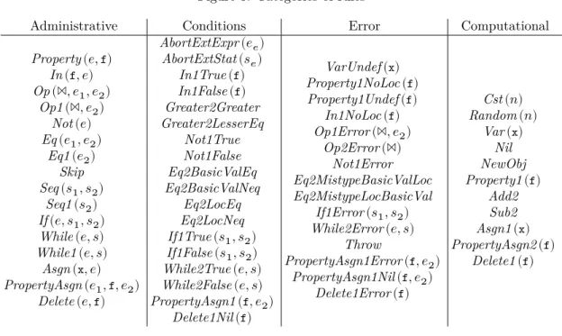
Figure ?? in Appendix ?? classifies the different rules of OWhile. As can be seen, very few rules fall into the computational category, which is the category yielding most of the abstraction effort. These categories are arbitrary and debatable as they just serve as a rough estimate on the amount of work needed to build the abstract semantics; for instance the third category of error rules has been added because a lot of rule falls into it, but they require the same amount of work to abstract than the condition rules. For instance, let us consider the two concrete rules for assignments:
Asgn(x, 𝑒)
𝑆, 𝑒 ⇓ 𝑟 𝑟,x∶=1⇓ 𝑟′
𝑆,x∶= 𝑒 ⇓ 𝑟′
Asgn1(x)
(𝑆, 𝑣),x∶=1⇓ write (𝑆, 𝑥, 𝑣)
The first rule Asgn (x, 𝑒) is an administrative rule: its definition does not depend on the implementation of states and its abstract version is identical. On the other hand, the rule Asgn1 (x) uses the concrete write operation, which does not straightforwardly translate into the abstract world: we do so by exhibiting its footprint. This leads to the following two abstract rules for assignment. In contrary to [?], we only give a local version of the rules: the abstract rules work with the frame rule (see next section). Note how compact the rule Asng1 (x) is, its context being implicit. Also note that although the concrete rule Asng1 (x) applies even if xis not defined in the state, we require it to be present in the abstract formula—eventually with the value ⊠. This solves the problem stated by Reynolds [?, Section 3.5], as the frame rule can no longer interfere with the resourcex.
Asgn(x, 𝑒) Φ, 𝑒 ⇓♯Φ′ Φ′,x∶= 1⇓♯Φ″ Φ,x∶= 𝑒 ⇓♯Φ″ Asgn1(x) (𝑀 ∣x= 𝑣̇ ♯0, 𝑣♯) ,x∶= 1⇓♯(𝑀 ∣x= 𝑣̇ ♯)
The only abstract rule of OWhile whose footprint updates the membrane is the rule NewObj, whose concrete and abstract rules follow. The concrete rule exhibit a fresh concrete location which has no associated reference 𝑙fresh(𝑆).f in the current state 𝑆. In the abstract rule, we create a new
location 𝑙 and declare it as fresh in the membrane: this ensures it to be different from anything present in the context. We also claim that we have write permission over this new location 𝑙 by adding a memory cell into the formula, leaving its fields undefined as in the concrete rule.
NewObj
𝑆, {} ⇓ (𝑆, 𝑙fresh(𝑆))
NewObj
(∅ | emp) , {} ⇓ (𝜈𝑙 | 𝑙 ↦ {_ ∶ ⊠} , 𝑙)
6.3. Interfering with the Frame Rule
The version of the frame rule which we use is recalled below.
Frame
Φ, 𝑡 ⇓♯Φ′
Φ𝑐⋆ Φ, 𝑡 ⇓.. ♯Φ𝑐 ⋆ Φ.. ′
To make sense, the abstract semantics has to keep interface (Φ) constant along the derivation. It would otherwise be possible to exhibit a context Φ𝑐 with a different behaviour in both sides. For instance, although Φ1 = (𝑙 → 𝑙 | 𝑙 ↦ {_ ∶ ⊠}) and Φ2 = (𝑙′→ 𝑙 ∣ 𝑙 ↦ {_ ∶ ⊠}) represent the same
Φ𝑐⋆ Φ.. 1 has an empty concretisation but not Φ𝑐⋆ Φ.. 2. Because of the frame rule, we can no longer replace a formula Φ by another Φ′ just because they represent the same concrete states.
In contrary to usual abstract interpretation, the subset ≼ of a pre-order which we consider is requested to be sound in any context Φ𝑐. The fact that this pre-order does not form a lattice—or that it is only a subset of a pre-order—can be surprising; but building a full-fledged lattice can be difficult. Furthermore, we actually do not need such hypotheses to prove the soundness of our approach: we have quotiented the formulae by the equivalent relation built from ≼, and we can complete the order ≼ by taking its transitive closure. The lattice usually requested by abstract interpretation only greatly helps in building analysers, but we are here only interested in building an abstract semantics.
Φ1≼ Φ2 ⟹ ∀Φ𝑐. 𝛾 (Φ𝑐⋆ Φ.. 1) ⊆ 𝛾 (Φ𝑐⋆ Φ.. 2)
Following Schmidt [?], meta rules are not mixed with abstract rules. We thus force the frame rule into the glue between rules by updating the function glue♯, as we did when adding the Weaken rule:
glue♯𝑖(⇓♯0) = {(Φ𝜎, 𝑡, Φ𝑟) ∣ ∃Φ′𝜎, Φ𝑐, Φ′𝑟. Φ𝜎≼ Φ𝑐⋆ Φ.. ′𝜎∧ Φ𝑐⋆ Φ.. ′𝑟≼ Φ𝑟∧ (Φ′𝜎, 𝑡, Φ′𝑟) ∈ apply𝑖(⇓ ♯ 0)}
Given a semantic context Φ𝜎, we are allowed to approximate it, then split it into the formula Φ′𝜎
which matches the rule application and a context Φ𝑐. We then run the rule on Φ′𝜎 to get Φ′𝑟, which
we consider in the frame Φ𝑐. We allow a final approximation to get Φ𝑟. The abstract states are not
always formulae, but can be extended formulae (see Section ??). Fortunately the operator ..⋆ and the pre-order ≼ can be adapted for extended formulae. We do not show the details here for space reasons. Let us consider the example of Asng1 (x): it is the rule taking care of the assignment just after the assigned expression has been computed; It takes an extended semantic context as argument, carrying the computed expression. It requires the variablexto stand in the input formula:
Asgn1(x)
(𝑀 ∣x= 𝑣̇ ♯0, 𝑣♯) ,x∶=
1⇓♯(𝑀 ∣x= 𝑣̇ ♯)
Given a semantic context Φ = (𝑀 ∣ 𝜙, 𝑣♯), there are two cases, whetherxappears in 𝜙. If it does not
appear, then the rule does not apply. Otherwise 𝜙 is on the formx= 𝑣̇ ♯0⋆ 𝜙′: we isolate xinto Φ =
(𝑀 ∣ 𝜙′) ..⋆ (𝑀′∣x= 𝑣̇ ♯
0, 𝑣♯), where 𝑀′= {ℎ → ℎ|ℎ ∈ codom (𝑀 )} is neutral with 𝑀 . The application
of the rule then returns after reapplying the context (𝑀 ∣ 𝜙′) ..⋆ (𝑀′∣x= 𝑣̇ ♯) = 𝜙′ ⋆ (𝑀 ∣.. x= 𝑣̇ ♯).
Let us now consider the example of Delete1 (f). This extended rule receives a location and updates its referenced object. Let us see how it behaves when received a summary node 𝑘 instead of a precise abstract location 𝑙 by giving it the semantic context Φ = (𝑘 → 𝑘 | 𝑘 ↦ {f∶ nil, _ ∶ ⊠} , 𝑘).
Delete1(f)
(𝑀 | 𝑙 ↦ {𝑜} , 𝑙) , delete1.f⇓♯(𝑀 ∣ 𝑙 ↦ remove♯(f, {𝑜}))
The abstract operation remove♯ writes ⊠ in the field f of the abstract object {𝑜}. Using a
materialization—the carried value being its entry point—we can build the following formula Φ′.
Φ ≼ Φ′= (𝑘 → 𝑙′+ 𝑘′∣ 𝑙′↦ {f∶ nil, _ ∶ ⊠} ⋆ 𝑘′↦ {f∶ nil, _ ∶ ⊠} , 𝑙′)
= (𝑘 → 𝑙′+ 𝑘′∣ 𝑘′↦ {f∶ nil, _ ∶ ⊠}) ..⋆ (𝑙′→ 𝑙′∣ 𝑙′↦ {f∶ nil, _ ∶ ⊠} , 𝑙′)
We can now apply the abstract rule Delete1 (f) on the first part to get the following. Φ″= (𝑘 → 𝑙′+ 𝑘′∣ 𝑘′↦ {f∶ nil, _ ∶ ⊠}) ..⋆ (𝑙′→ 𝑙′∣ 𝑙′↦ {_ ∶ ⊠} , 𝑙′)
= (𝑘 → 𝑙′+ 𝑘′∣ 𝑙′↦ {_ ∶ ⊠} ⋆ 𝑘′↦ {f∶ nil, _ ∶ ⊠} , 𝑙′)
We can now either continue with this result, which is a strong update over a local location identifier 𝑙′. But we might want to diminish the size of the membrane: let us see what happen if we summarize
6.4. Correctness
The correctness relies on the concretisation 𝛾 of formulae. Concretisation of formula is defined through a predicate ⊨ shown in Figure ??; this predicate is parametrized by a valuation 𝜌 ∶ LLoc♯⇀
Loc ∧ KLoc♯ ⇀ 𝒫 (Loc) of abstract locations to concrete locations. The difficult part stands in the concretisation of objects, where abstract values 𝑣♯can represent an undefined concrete value if ⊠ ⊑ 𝑣♯.
We do not show the definition of the concretisation function of objects, but it comes with no surprise. The set 𝑅 is used to store the reserved variables: x = ⊠ states that the variablė x is not in the environment, but it still reserves the resourcexto be sound with the frame rule; this fact is stored by 𝑅. The concretisation 𝛾 (Φ) of a formula Φ is then a projection of this predicate:
(𝐸, 𝐻) ∈ 𝛾 ((𝑀 | 𝜙)) ⟺ ∃𝜌, 𝑅. (𝐸, 𝑅, 𝐻) ⊨𝜌𝜙
(𝐸, 𝑅, 𝐻) ⊨𝜌emp ⟺ 𝐸 = 𝑅 = 𝐻 = ∅
(𝐸, 𝑅, 𝐻) ⊨𝜌𝜙1⋆ 𝜙2 ⟺ ∃𝐸1, 𝑅1, 𝐻1, 𝐸2, 𝑅2, 𝐻2. 𝐸 = 𝐸1⊎ 𝐸2∧ 𝑅 = 𝑅1⊎ 𝑅2 ∧ dom (𝐸1), dom (𝐸2), 𝑅1, and 𝑅2 are disjoint pairwise
∧ 𝐻 = 𝐻1⊎ 𝐻2∧ dom (𝐻1) ∩ dom (𝐻2) = ∅ ∧ ∀𝑖. (𝐸𝑖, 𝑅𝑖, 𝐻𝑖) ⊨𝜌𝜙𝑖 (𝐸, 𝑅, 𝐻) ⊨𝜌x= 𝑣̇ ♯ ⟺ 𝐻 = ∅ ∧ (⊠ ⊑ 𝑣♯∧ 𝐸 = ∅ ∧ 𝑅 = {x} ∨ ∃𝑣 ∈ 𝛾𝜌(𝑣♯) ∧ 𝐸 = {(x, 𝑣)} ∧ 𝑅 = ∅) (𝐸, 𝑅, 𝐻) ⊨𝜌𝑙 ↦ {𝑜} ⟺ 𝐸 = 𝑅 = ∅ ∧ ∃𝑜0∈ 𝛾𝜌({𝑜}) . 𝐻 = {(𝜌 (𝑙) ,f, 𝑜0)} (𝐸, 𝑅, 𝐻) ⊨𝜌𝑘 ↦ {𝑜} ⟺ 𝐸 = 𝑅 = ∅ ∧ ∃ (𝑜𝑖) ∈ (𝛾𝜌({𝑜})) 𝜌(𝑘) . 𝐻 = ⋃ 𝑙𝑖∈𝜌(𝑘) {(𝜌 (𝑙) ,f, 𝑜𝑖)}
Figure 3: Definition of the entailment predicate ⊨𝜌.
The approach for correctness is the same than in [?]: we require every abstract rule to be locally correct, i.e., their transfer functions (noted for axioms ax and ax♯ in the respective concrete and
abstract semantics) and side conditions (noted cond and cond♯) follow the corresponding concrete rules, taking into account a potential context. The local correctness conditions over transfer functions and side conditions of axiom rules follow—the correctness of other types of rule is very similar. Because of the context in the side condition, it is possible to have a rule whose side condition holds, but whose semantic context does not match the transfer function: this amounts to say that the construction of a derivation can be blocked if some resources are lacking in the original semantic context. We shall not extend on this technical matter. We can infer from these local properties the global correctness.
∀𝑆, Φ, Φ𝑐. 𝑆 ∈ 𝛾 (Φ𝑐⋆ Φ) ⟹ ax (𝑆) ∈ 𝛾 (Φ.. 𝑐⋆ ax.. ♯(Φ))
∀𝑖, 𝑆, Φ, Φ𝑐. 𝑆 ∈ 𝛾 (Φ𝑐⋆ Φ) ⟹ cond.. 𝑖(𝑆) ⟹ cond ♯ 𝑖(Φ)
Property 1 (Global Correctness) Let 𝑡 be a term, 𝑆 and 𝑆′ be states, and Φ and Φ′ formulae. Given the local correctness, if 𝑆 ∈ 𝛾 (Φ), 𝑆, 𝑡 ⇓ 𝑆′, and Φ, 𝑡 ⇓♯Φ′ then 𝑆′∈ 𝛾 (Φ′).
In other words, abstract derivations can not miss concrete executions: our abstract semantics is sound.
7.
Related Work
This work directly follows from [?], which only focussed on abstract interpretation and how to make a Coq development scale up to big operational semantics such as JavaScript’s. This previous work
came with a Coq development containing some generic analysers, while the current work only focuses at building an abstract domain compatible with the frame rule. There have been works aiming at providing formally verified analysers on languages other than JavaScript such as [?], but these involve a lot of Coq development and we hope to get to a comparatively lighter development for JavaScript. We aim at diving the work of [?] to a fully Coq-verified abstract interpreter.
There have been some work about mixing abstract interpretation and separation logic, such as [?] or [?], but few provide an abstract semantics compatible with the frame rule able to express the abstractions of shape analysis. The lattices constructed by these works are based on a disjunctive completion of a formula order, which can easily explode in size. Our mechanism provides a protection against these explosions through summarizations, with the cost of potentially big imprecision.
The logic of [?] is very close to this work; their domain is a disjunctive completion of formulae separated at the field level of objects as we did. Locations and fields are both abstracted by either singletons or summary nodes. However, the frame rule is not mentioned, which removes the need of membranes. They carry a set of formulae storing information about the respective inclusion of the concretisations of summary nodes. Their domain is ordered and equipped with a join and a widening operator with an algorithm compatible with the concretisation function.
The same authors previously developped [?] based on separation logic; this work focusses on inductively defined shapes and is able to express and analyse complex structures such as red-black trees. To increase the efficiency of the analyse, they developed a way to change the point of view of these shapes: for instance, a doubly linked list can be defined either by following next or previous
fields. As with this work, the order relation, are defined through an algorithm compatible with the concretisation function, and they similarly defined joins and widenings by an algorithm.
Inductively defined structures have also been examined in [?], which uses abduction to determine the weakest precondition wielding safety or termination of the analysed program. They provide heuristics to infer how to generalize predicates, as well as a running tool. However, their heuristics rely on the syntax of their toy language (comparable to OWhile): scaling such an analyser up to JavaScript might require to look for much complex heuristics, and we think that an approach guided directly by the language semantics can reduce the amount of work to get a certified analyser.
8.
Conclusion and Future Works
We have presented a program logic for JavaScript heaps, based on separation logic and integrating ideas from shape analysis. We have expressed this logic within a framework of certified abstract interpretation. The goal is to scale up the logic to the size of JavaScript’s semantics, resulting in an abstract semantics for JavaScript of reasonable size, and eventually certified analysers for JavaScript. The particular problem addressed in this paper is that of integrating the frame rule to existing abstract interpretation framework, which is known to be a difficult problem.
Our approach is precise enough to get interesting results on real-world programs, whilst being simple enough to be able to scale it up to a certified abstract semantics of JavaScript. This work is part of a larger project which aims at building certified static analyses based on the JSCert [?] formal semantics of JavaScript.
We have focussed on how to build an abstract semantics, and not on how to build analysers. The abstract domains that arise from our logic are less structured than usual abstract domains, which means that an analyser will be less guided by the abstract interpretation framework. There is thus room for further research into the construction of efficient join and widening operators for abstract domains combining separation and summarization. Furthermore, the frame rule allows to individually analyse functions or recurrent programs; it is thus natural to look for strategies to choose and separately analyse these programs. We have observed that analysing a program without starting from the right resources can lead to big approximations, or to the inability to analyse. Techniques
𝑠 ∶∶= skip | 𝑠1; 𝑠2 | if 𝑒 𝑠1𝑠2 | while 𝑒 𝑠 | throw |x∶= 𝑒 | 𝑒1.f∶= 𝑒2 | delete 𝑒.f (a) Statements 𝑒 ∶∶= 𝑛 ∈ ℤ | ? |x∈ Var | nil | {} | 𝑒.f |f in𝑒 | ¬ 𝑒 | = 𝑒1 𝑒2 |1 𝑒1 𝑒2 (1 ∈ {>, +, −}) (b) Expressions 𝑠𝑒∶∶= ;1𝑠2 | if1𝑠1𝑠2 | while1𝑒 𝑠 | while2𝑒 𝑠 |x∶=1 |.f∶=1 𝑒2 |.f∶=2 | delete1.f (c) Extended statements 𝑒𝑒∶∶=.f |f in1 |11𝑒2 |12 | ¬1 | =1 𝑒2 | =2 (d) Extended expressions
Figure 4: Complete syntax of the OWhile language
like bi-abduction may be relevant to build efficient oracles for our certified analysers.
A.
Concrete Semantics
Figure ?? presents the complete syntax of OWhile, which includes extended terms. These extended terms carry intermediary results, and are thus associated with specific kinds of extended semantic contexts, carrying additional values. The concrete rules follow. These rules makes use of functions such as read and write which perform some semantic manipulation; their semantics is usual and we do not explicit them. Section ?? categorizes rules into four different kinds of categories; Figure ?? shows where all the rules of this semantics fall. As can be seen, the categories are more or less identical in size, with the notable exception of the computational rules, which are the most difficult to abstract.
AbortExtExpr(𝑒𝑒) 𝜎, 𝑒𝑒⇓ Err 𝜎 = Err AbortExtStat(𝑠𝑒) 𝜎, 𝑠𝑒⇓ Err 𝜎 = Err Cst(𝑛) 𝑆, 𝑛 ⇓ (𝑆, 𝑛) Random(𝑛) 𝑆, ? ⇓ (𝑆, 𝑛) Var(x) 𝑆,x⇓ (𝑆, read (𝑆,x)) x∈ dom (𝑆) VarUndef(x) 𝑆,x⇓ Err x∉ dom (𝑆)
Nil 𝑆, nil ⇓ (𝑆, 𝑙0) NewObj 𝑆, {} ⇓ (𝑆, 𝑙fresh(𝑆)) Property(𝑒, f) 𝑆, 𝑒 ⇓ 𝑟 𝑟,.f⇓ 𝑟′ 𝑆, 𝑒.f⇓ 𝑟′ Property1(f) (𝑆, 𝑙𝑖),.f⇓ (𝑆, read (𝑆, 𝑙𝑖.f)) 𝑙 𝑖.f∈ dom (𝑆) Property1NoLoc(f) (𝑆, 𝑛),.f⇓ Err Property1Undef(f) (𝑆, 𝑙𝑖),.f⇓ Err 𝑙 𝑖.f∉ dom (𝑆) In(f, 𝑒) 𝑆, 𝑒 ⇓ 𝑟 𝑟,f in1⇓ 𝑟′ 𝑆,e in𝑓 ⇓ 𝑟′ In1True(f) (𝑆, 𝑙𝑖),f in 1⇓ (𝑆, 1) 𝑙𝑖.f∈ dom (𝑆) In1NoLoc(f) (𝑆, 𝑛),f in1⇓ Err In1False(f) (𝑆, 𝑙𝑖),f in 1⇓ (𝑆, 0) 𝑙𝑖.f∉ dom (𝑆) Op(1, 𝑒1, 𝑒2) 𝑆, 𝑒1⇓ 𝑟 𝑟,11 𝑒2⇓ 𝑟′ 𝑆,1 𝑒1 𝑒2⇓ 𝑟′ Op1(1, 𝑒2) 𝑆, 𝑒2⇓ 𝑟 (𝑛1, 𝑟),12⇓ 𝑟′ (𝑆, 𝑛1),11𝑒2⇓ 𝑟′ Op1Error(1, 𝑒2) (𝑆, 𝑙𝑖),1 1 𝑒2⇓ Err Op2Error(1) (𝑛1, (𝑆, 𝑙𝑗)),12⇓ Err Add2 (𝑛1, (𝑆, 𝑛2)), +2⇓ (𝑆, 𝑛1+ 𝑛2) Sub2 (𝑛1, (𝑆, 𝑛2)), −2⇓ (𝑆, 𝑛1− 𝑛2) Greater2Greater (𝑛1, (𝑆, 𝑛2)), >2⇓ (𝑆, 1) 𝑛1> 𝑛2 Greater2LesserEq (𝑛1, (𝑆, 𝑛2)), >2⇓ (𝑆, 0) 𝑛1≤ 𝑛2 Not(𝑒) 𝑆, 𝑒 ⇓ 𝑟 𝑟, ¬1⇓ 𝑟′ 𝑆, ¬ 𝑒 ⇓ 𝑟′ Not1True (𝑆, 𝑛), ¬1⇓ (𝑆, 0) 𝑛 ≠ 0 Not1False (𝑆, 𝑛), ¬1⇓ (𝑆, 1) 𝑛 = 0 Not1Error (𝑆, 𝑙), ¬1⇓ Err Eq(𝑒1, 𝑒2) 𝑆, 𝑒1⇓ 𝑟 𝑟, =1 𝑒2⇓ 𝑟′ 𝑆, = 𝑒1 𝑒2⇓ 𝑟′ Eq1(𝑒2) 𝑆, 𝑒2⇓ 𝑟 (𝑣1, 𝑟), =2⇓ 𝑟′ (𝑆, 𝑣1), =1 𝑒2⇓ 𝑟′ Eq2BasicValEq (𝑛1, (𝑆, 𝑛2)), =2⇓ (𝑆, 1) 𝑛1= 𝑛2 Eq2BasicValNeq (𝑛1, (𝑆, 𝑛2)), =2⇓ (𝑆, 0) 𝑛1≠ 𝑛2 Eq2LocEq (𝑙𝑖, (𝑆, 𝑙𝑗)), = 2⇓ (𝑆, 1) 𝑙𝑖= 𝑙𝑗 Eq2LocNeq (𝑙𝑖, (𝑆, 𝑙𝑗)), = 2⇓ (𝑆, 0) 𝑙𝑖≠ 𝑙𝑗 Eq2MistypeBasicValLoc (𝑛1, (𝑆, 𝑙𝑗)), =2⇓ Err Eq2MistypeLocBasicVal (𝑙𝑖, (𝑆, 𝑛 2)), =2⇓ Err Skip 𝑆, skip ⇓ 𝑆 Seq(𝑠1, 𝑠2) 𝑆, 𝑠1⇓ 𝑟 𝑟, ;1𝑠2⇓ 𝑟′ 𝑆, 𝑠1; 𝑠2⇓ 𝑟′ Seq1(𝑠2) 𝑆, 𝑠2⇓ 𝑟 𝑆, ;1𝑠2⇓ 𝑟 Throw 𝑆, throw ⇓ Err
If(𝑒, 𝑠1, 𝑠2) 𝑆, 𝑒 ⇓ 𝑟 𝑟, if1𝑠1𝑠2⇓ 𝑟′ 𝑆, if 𝑒 𝑠1𝑠2⇓ 𝑟′ If1True(𝑠1, 𝑠2) 𝑆, 𝑠1⇓ 𝑟 (𝑆, 𝑛), if1𝑠1𝑠2⇓ 𝑟 𝑛 ≠ 0 If1False(𝑠1, 𝑠2) 𝑆, 𝑠2⇓ 𝑟 (𝑆, 𝑛), if1𝑠1𝑠2⇓ 𝑟 𝑛 = 0 If1Error(𝑠1, 𝑠2) (𝑆, 𝑙𝑖), if 1𝑠1𝑠2⇓ Err While(𝑒, 𝑠) 𝑆, while1𝑒 𝑠 ⇓ 𝑟 𝑆, while 𝑒 𝑠 ⇓ 𝑟 While1(𝑒, 𝑠) 𝑆, 𝑒 ⇓ 𝑟 𝑟, while1𝑒 𝑠 ⇓ 𝑟′ 𝑆, while1𝑒 𝑠 ⇓ 𝑟′ While2True(𝑒, 𝑠) 𝑆, 𝑠 ⇓ 𝑟 𝑟, while1𝑒 𝑠 ⇓ 𝑟′ (𝑆, 𝑛), while2𝑒 𝑠 ⇓ 𝑟′ 𝑛 ≠ 0 While2False(𝑒, 𝑠) (𝑆, 𝑛), while2𝑒 𝑠 ⇓ 𝑆 𝑛 = 0 While2Error(𝑒, 𝑠) (𝑆, 𝑙𝑖), while 2𝑒 𝑠 ⇓ Err Asgn(x, 𝑒) 𝑆, 𝑒 ⇓ 𝑟 𝑟,x∶=1⇓ 𝑟′ 𝑆,x∶= 𝑒 ⇓ 𝑟′ Asgn1(x) (𝑆, 𝑣),x∶=1 ⇓ write (𝑆, 𝑥, 𝑣) PropertyAsgn(𝑒1, f, 𝑒2) 𝑆, 𝑒1⇓ 𝑟 𝑟,.f∶=1 𝑒2⇓ 𝑟′ 𝑆, 𝑒1.f∶= 𝑒2⇓ 𝑟′ PropertyAsgn1(f, 𝑒2) 𝑆, 𝑒2⇓ 𝑟 (𝑙𝑖, 𝑟),.f∶= 2⇓ 𝑟′ (𝑆, 𝑙𝑖),.f ∶= 1 𝑒2⇓ 𝑟′ PropertyAsgn1Error(f, 𝑒2) (𝑆, 𝑛),.f∶=1 𝑒2⇓ Err PropertyAsgn1Nil(f, 𝑒2) (𝑆, 𝑙0),.f∶= 1 𝑒2⇓ Err PropertyAsgn2(f) (𝑙𝑖, (𝑆, 𝑣)),.f∶= 2⇓ write (𝑆, 𝑙𝑖.f, 𝑣) Delete(𝑒, f) 𝑆, 𝑒 ⇓ 𝑟 𝑟, delete1.f⇓ 𝑟′ 𝑆, delete 𝑒.f⇓ 𝑟′ Delete1(f) (𝑆, 𝑙𝑖), delete 1.f⇓ remove (𝑆, 𝑙𝑖.f) Delete1Error(f) (𝑆, 𝑛), delete1.f⇓ Err Delete1Nil(f) (𝑆, 𝑙0), delete 1.f⇓ Err
B. Pre-order over Formulae
As said in Section ??, we are looking for a relation ≼ which respects the frame property: Φ1≼ Φ2 ⟹ ∀Φ𝑐. 𝛾 (Φ𝑐⋆ Φ.. 1) ⊆ 𝛾 (Φ𝑐⋆ Φ.. 2)
The empty relation would be correct; however, it would not be useful as it allows no transformation to the formulae: we would like to account for materializations and summarizations. We define our relation ≼ by an algorithm taking two abstract heaps Φ1= (𝑀1| 𝜙1) and Φ2= (𝑀2| 𝜙2) and returning
true if it successfully proved the above property. However, the inclusion of the concretisations does
not necessarily yield the pre-order relation. We have not focused on the efficiency of this algorithm.
B.1.
Example
To illustrate our comparison algorithm, let us consider the following two formulae to get Φ1≼ Φ2.
Φ1= (𝑘0→ 𝑘, 𝑙0→ 𝑙 |x= 𝑙 ⊔ 𝑘 ⋆ 𝑘 ↦ {̇ f∶ ⊥,g∶ 𝑙, _ ∶ ⊠} ⋆ 𝑙 ↦ {f∶ 𝑙, _ ∶ ⊠})
Figure 5: Categories of rules
Administrative Conditions Error Computational
Property (𝑒,f) In (f, 𝑒) Op (1, 𝑒1, 𝑒2) Op1 (1, 𝑒2) Not (𝑒) Eq (𝑒1, 𝑒2) Eq1 (𝑒2) Skip Seq (𝑠1, 𝑠2) Seq1 (𝑠2) If (𝑒, 𝑠1, 𝑠2) While (𝑒, 𝑠) While1 (𝑒, 𝑠) Asgn (x, 𝑒) PropertyAsgn (𝑒1,f, 𝑒2) Delete (𝑒,f) AbortExtExpr (𝑒𝑒) AbortExtStat (𝑠𝑒) In1True (f) In1False (f) Greater2Greater Greater2LesserEq Not1True Not1False Eq2BasicValEq Eq2BasicValNeq Eq2LocEq Eq2LocNeq If1True (𝑠1, 𝑠2) If1False (𝑠1, 𝑠2) While2True (𝑒, 𝑠) While2False (𝑒, 𝑠) PropertyAsgn1 (f, 𝑒2) Delete1Nil (f) VarUndef (x) Property1NoLoc (f) Property1Undef (f) In1NoLoc (f) Op1Error (1, 𝑒2) Op2Error (1) Not1Error Eq2MistypeBasicValLoc Eq2MistypeLocBasicVal If1Error (𝑠1, 𝑠2) While2Error (𝑒, 𝑠) Throw PropertyAsgn1Error (f, 𝑒2) PropertyAsgn1Nil (f, 𝑒2) Delete1Error (f) Cst (𝑛) Random (𝑛) Var (x) Nil NewObj Property1 (f) Add2 Sub2 Asgn1 (x) PropertyAsgn2 (f) Delete1 (f)
Our algorithm starts by splitting Φ1 to remove disjunctions in the values of variables and abstract
locations 𝑙. In the example x = 𝑙 ⊔ 𝑘 can be split intȯ x = 𝑙 anḋ x = 𝑘 to get the two formulaė Φ1,𝑎and Φ1,𝑏below. This is sound as the disjunction ⊔ we chose for values does not loose precision:
∀Φ𝑐. 𝛾 (Φ𝑐 ⋆ Φ.. 1) = 𝛾 (Φ𝑐⋆ Φ.. 1,𝑎) ∪ 𝛾 (Φ𝑐⋆ Φ.. 1,𝑏).
Φ1,𝑎= (𝑘0→ 𝑘, 𝑙0→ 𝑙 |x= 𝑙 ⋆ 𝑘 ↦ {̇ f∶ ⊥,g∶ 𝑙, _ ∶ ⊠} ⋆ 𝑙 ↦ {f∶ 𝑙 ⊔ 𝑘, _ ∶ ⊠})
Φ1,𝑏= (𝑘0→ 𝑘, 𝑙0→ 𝑙 |x= 𝑘 ⋆ 𝑘 ↦ {̇ f∶ ⊥,g∶ 𝑙, _ ∶ ⊠} ⋆ 𝑙 ↦ {f∶ 𝑙 ⊔ 𝑘, _ ∶ ⊠})
Let us focus on Φ1,𝑎. We look for a function 𝜓 translating identifiers of the formula Φ1,𝑎 to those
of Φ2 in order to match Φ1,𝑎 with Φ2. Here the function 𝜓 mapping 𝑙 to 𝑙′ and 𝑘 to 𝑘′ is enough.
Applying the rewriting 𝜓 over Φ1,𝑎 follows the same rules as the 𝛼-renaming and the summarization
presented in Sections ?? and ??—which is why summarizations are compatible with this pre-order: 𝜓 (Φ1,𝑎) = (𝑘0→ 𝑘′, 𝑙
0→ 𝑙′∣x= 𝑙̇ ′⋆ 𝑘′↦ {f∶ ⊥,g∶ 𝑙, _ ∶ ⊠} ⋆ 𝑙′↦ {f∶ 𝑙′⊔ 𝑘′, _ ∶ ⊠})
The summary node 𝑘 has an incoherence: every concrete location represented by 𝑘 is supposed to have a field f represented by ⊥, which is not possible: the only possible concretisation of 𝑘 is the empty set. We can thus safely remove 𝑘 from the formula:
Φ′
1,𝑎= (𝑘0→ ∅, 𝑙0→ 𝑙′∣x= 𝑙̇ ′⋆ 𝑙′↦ {f∶ 𝑙′, _ ∶ ⊠})
At this point, we compare the inner scope of Φ′
1,𝑎 with the one of Φ2: the latter has
an additional summary node 𝑘′. We can easily ignore such a summary node as it can
represent an empty set of concrete locations; we thus rewrite 𝑘′ into ∅ in Φ
2 to get Φ′2 =
(𝑘0→ 𝑙′, 𝑙0→ 𝑙′∣x= 𝑙̇ ′⋆ 𝑙′↦ {f∶ 𝑙′⊔ nil, _ ∶ ⊠}). We now compare the values in the membrane,
the variables, and the objects; which we can check are greater in Φ′
2 for any corresponding in Φ′1,𝑎.
We have successfully found a 𝜓 leading to the conclusion ∀Φ𝑐. 𝛾 (Φ𝑐⋆ Φ.. 1,𝑎) ⊆ 𝛾 (Φ𝑐⋆ Φ.. 2).
In the case of Φ1,𝑏we can perform a materialization, as the have an entry point to a summary node x= 𝑘. But this generates a subformula 𝑙̇ ′↦ {f∶ ⊥,g∶ 𝑙, _ ∶ ⊠}, which has an empty concretisation
as the reference 𝑙′.fshould be ⊥. We can conclude that Φ
1,𝑏has an empty concretisation, and thus