U N IV E R S IT E D E
SHERBROOKE
Faculte de genie
Departement de genie civil
Developpement d ’un nouveau dispositif piezoelectrique d ’essai d ’impulsion
et caracterisation des sols avec les ondes de cisaillement
These de doctorat es sciences appliquees Speciality: genie civil
Deyab GAMAL EL-DEAN
1*1
Library and
Archives Canada
Published Heritage
Branch
3 9 5 W ellingt on S tr e e t Ottaw a ON K 1 A 0 N 4 C a n a d aBibliotheque et
Archives Canada
Direction du
Patrimoine de I'edition
3 9 5 , rue Wellington O ttaw a ON K 1 A 0 N 4 C a n a d aYour file Votre reference ISBN: 978-0-494-37971-4 Our file Notre reference ISBN: 978-0-494-37971-4
NOTICE:
The author has granted a non
exclusive license allowing Library
and Archives Canada to reproduce,
publish, archive, preserve, conserve,
communicate to the public by
telecommunication or on the Internet,
loan, distribute and sell theses
worldwide, for commercial or non
commercial purposes, in microform,
paper, electronic and/or any other
formats.
AVIS:
L'auteur a accorde une licence non exclusive
permettant a la Bibliotheque et Archives
Canada de reproduire, publier, archiver,
sauvegarder, conserver, transmettre au public
par telecommunication ou par Nntemet, preter,
distribuer et vendre des theses partout dans
le monde, a des fins commerciales ou autres,
sur support microforme, papier, electronique
et/ou autres formats.
The author retains copyright
ownership and moral rights in
this thesis. Neither the thesis
nor substantial extracts from it
may be printed or otherwise
reproduced without the author's
permission.
L'auteur conserve la propriete du droit d'auteur
et des droits moraux qui protege cette these.
Ni la these ni des extraits substantiels de
celle-ci ne doivent etre imprimes ou autrement
reproduits sans son autorisation.
In compliance with the Canadian
Privacy Act some supporting
forms may have been removed
from this thesis.
While these forms may be included
in the document page count,
their removal does not represent
any loss of content from the
thesis.
Conformement a la loi canadienne
sur la protection de la vie privee,
quelques formulaires secondaires
ont ete enleves de cette these.
Bien que ces formulaires
aient inclus dans la pagination,
il n'y aura aucun contenu manquant.
■ W— U N IV E R S IT E D E
1 1 SHERBROOKE
Faculte de genie
Departement de genie civil
DEVELOPMENT OF A NEW PIEZOELECTRIC PULSE TESTING DEVICE
AND SOIL CHARACTERIZATION USING SHEAR WAVES
Deyab GAMAL EL-DEAN
Dissertation submitted in partial fulfillment
of the requirements for the degree of
Doctor of Philosophy
in
Civil Engineering
ABSTRACT
The shear-wave velocity (Vs) is a fundamental parameter that correlates well to soil properties, and is important in m any applications. Hence, there is an increasing interest in using shear-wave velocity to define soil state (void ratio, effective stresses, density, liquefaction potential, etc). The global idea of this research is to establish correlations between shear wave velocity and the basic soil parameters that can be used to evaluate soil properties and estimate its strength and deformation characteristics. These relationships will also allow the interpretation o f in situ geophysical measurements in terms o f the design parameters o f soil. The needed reliable correlations should be based on accurate measurements.
In this research, it has been proven that the bender-elements method, which is widely used to measure shear wave velocity o f soil in laboratory setups, suffers from fundamental and interpretative problems. Consequently, its results are controversial and m ight give highly erroneous values. After thorough numerical and laboratory investigations, a new piezoelectric pulse testing device (Ring Actuators Setup) was invented and developed in this research. This setup is composed o f two units (emitter and receiver) and is capable o f measuring shear and compression wave velocities o f soil specimens. It is a completely new, versatile, advanced and accurate setup. W ith this device, m any problems of pulse tests, which make interpretation o f results difficult and ambiguous, were solved. The ring actuators setup overcomes wave reflections at boundaries (end-caps and sides), sample disturbance, weak shear coupling between soil and device (interaction) as well as the fixation problems, low resonant frequency and limited input voltage o f the existing device. The development stages o f this device were also useful in reaching important findings for building robust setups. This device was implemented in the top cap and pedestal of a large oedometer cell. This setup was also used with Proctor mold as well as other fabricated molds. Many pulse tests were carried out on different soil types using this device. Shear and compression wave velocities could be accurately m easured at dry and partially saturated conditions under very low to high pressures. The compaction curves, in terms o f Vs and water content, were drawn for two soil types using the new device. In addition, some correlations between Vs and soil parameters were obtained.
Numerical sim ulations and analytical studies were also carried out in this research in order to study the characteristics o f elastic waves transmission through soil specimens in different laboratory setups. The bender-elements and the ring actuators models were studied. The interpretation problems o f pulse tests were thoroughly investigated numerically and experimentally. In this research, the reason of ‘near-field effect’ in pulse tests, which causes significant errors in the interpretation process, could be discovered. The parameters that control this phenom enon could be stated and their effects on the test results were quantified. In light o f these results, a new criterion for carrying out and interpreting pulse tests was established. Also, a simple interpretation method is introduced (Energy Rise-Time). Furthermore, the dispersive nature o f pulse tests was proven num erically and experimentally. Moreover, it was concluded that the shear wave velocity from pulse tests should be interpreted in the frequency domain, w hich renders ‘the simple methods o f interpretation’ inaccurate. Based on these findings, a new interpretation technique for pulse tests using W igner-Ville transform was presented. It was successfully used to interpret the numerical and physical pulse test results in this study.
The last part o f this research concerns soil characterization using shear wave velocity. Establishing correlations betw een Vs and soil parameters that can be used for soil characterization may be achieved in laboratory using piezoelectric devices, as mentioned above, or by deriving relationships between Vs and in situ test indices. In this research, the second approach was also exam ined for gravelly sands. Results o f the comprehensive field testing program for the natural soil and the embankment materials (fill) at Peribonka dam site were used to achieve this goal. Thorough interpretations and analyses were carried out for these tests in order to derive correlations between each o f CPTu and SPT indices and the in- situ F r measurements. Several important relationships and conclusions for soil characterization using shear waves could be reached. These correlations are useful for soil characterization not only at this site, but at other sites o f similar soil composition.
RESUM E
La vitesse de l’onde de cisaillement (Vs) est un parametre fondamental qui correspond bien aux proprietes de sol, et est important dans beaucoup d'applications. Par consequent, il y a un interet croissant a Lemploi de la vitesse de l’onde de cisaillement pour definir l'etat de sol (indice des vides, les contraintes effectives, la densite, le potentiel de liquefaction, etc). L'idee globale de cette recherche est d'etablir des correlations entre la vitesse de l ’onde de cisaillement et les parametres de base de sol qui peuvent etre employes pour evaluer les proprietes du sol et estimer ses caracteristiques de resistance et de deformation. Ces rapports pennettront egalement d ’interpreter des mesures geophysiques in situ en termes de parametres de conception de sol. Les correlations fiables necessaires devraient etre basees sur des mesures precises.
Dans cette recherche, on a prouve que la methode des languettes piezoceramiques (bender-elements), largement repandue pour mesurer la vitesse de l ’onde de cisaillement du sol dans des installations de laboratoire, souffre de problemes fondamentaux et interpretatifs. En consequence, ses resultats sont controverses et pourraient donner des valeurs fortement incorrectes. Apres des investigations numeriques et experimentales poussees, un nouveau dispositif piezoelectrique, installation des actuateurs d'anneau (Ring Actuators Setup), pour effectuez les essais d ’impulsion a ete invente et developpe dans cette recherche. Cette installation se compose de deux unites (emetteur et recepteur) et est capable de mesurer des vitesses de l’onde de cisaillem ent (Vs) et de compression ( Vp) des specimens de sol. C’est une installation completement nouvelle, souple, avancee et precise. Avec ce dispositif, plusieurs problemes d'essais d'impulsion, qui rendent l'interpretation des resultats difficile et ambigue, ont ete resolus. L ’installation de Ring Actuators surmonte les reflexions de l’onde aux frontieres (les extremites et les cotes), la perturbation d'echantillon, la faible interaction de cisaillement entre le sol et le dispositif ainsi que les problemes de fixation, la basse frequence de resonance et la tension d'entree limitee du dispositif existant. Les etapes de developpement de ce dispositif sont egalem ent etaient utiles en obtenant des resultats importants afin de construire des installations robustes. Ce dispositif a ete mis en application dans le cap et le piedestal d'une grande cellule d'oedometre. Cette installation a ete egalement employee avec le moule de Proctor comme d'autres moules fabriques. Beaucoup d'essais d'impulsion ont ete effectues sur differents types de sol a l'aide de ce dispositif. Des vitesses de l ’onde de cisaillement et de compression ont pu etre exactement mesurees a des conditions seches et partiellement saturees, sous de tres basses ou hautes pressions. Les courbes de compactage, en
termes de Vs et la teneur en eau, ont ete dessinees pour deux types de sol a l'aide du nouveau dispositif. En plus, quelques correlations entre Vs et les parametres de sol ont ete obtenus.
Des simulations numeriques et des etudes analytiques ont egalement ete effectuees dans mes travaux de recherche afin d'etudier les caracteristiques de la transmission de l ’onde elastique a travers des specimens de sol dans differentes installations de laboratoire. Des modeles des languettes piezoceramiques et des actuateurs d ’anneau ont ete etudies. Les problemes d'interpretation des essais d'impulsion ont ete etudies a fond, numeriquement et experimentalement. Dans cette recherche, les raisons du champ proche (near-field effects) en essais d'impulsion, qui causent des erreurs importantes dans le procede d'interpretation, pourraient etre decouvertes. Les parametres qui commandent ce phenomene pourraient etre enonces et leurs effets sur les resultats d'essai ont ete mesures.
A
la lumiere de ces resultats, un nouveau critere pour effectuer et interpreter des essais d'impulsion a ete etabli. En outre, une methode simple d'interpretation est presentee (temps de montee d'energie). De plus, la nature dispersive des essais d'impulsion a ete prouvee numeriquement et experimentalement. D'ailleurs, on a conclu que la vitesse de vague de cisaillement des essais d'impulsion devrait etre interpretee dans le domaine de frequence, qui rend les methodes simples d'interpretation imprecises. Basee sur ces resultats, une nouvelle technique d'interpretation pour des essais d'impulsion employant Wigner-Ville Transforme a ete presentee. Elle a ete utilisee avec succes pour interpreter les resultats d'essai physiques et numeriques d'impulsion.La derniere partie de cette recherche concerne la caracterisation de sol en utilisant la vitesse de l’onde de cisaillement. L'etablissement des correlations entre Vs et les parametres de sol, qui peuvent etre employes pour la caracterisation de sol, peut etre realise dans le laboratoire a l'aide de dispositifs piezoelectriques, comme mentionne ci-dessus, ou par derivation des relations entre Vs et les parametres d'essai in situ. Dans cette recherche, la deuxieme approche a ete egalement examinee pour les sables graveleux. Des resultats du programme complet d'essai sur le terrain, pour le sol naturel et les materiaux de barrage a T emplacement du barrage de Peribonka, ont ete employes pour realiser ce but. Les interpretations et les analyses completes ont ete effectuees pour ces essais afin de deriver des correlations entre chacune d'indice de CPTu et de SPT et des mesures de Vs in situ. Plusieurs relations et conclusions importantes pour la caracterisation du sol par les ondes de cisaillement ont pu etre tirees. Ces correlations sont utiles pour la caracterisation de sol non seulement a cet emplacement mais aux autres emplacements de composition de sol semblable.
D E D IC A T IO N
To tLe AeseaACieAS and engineeAS u/Lo appAeCiate tLe boiue op science and
knowledge.
To my belobed paAentS wLo pabouAed me obeA tLemSelbeS and Labe giben me a il
wLat tLey Could.
"My
LoAd.! TfeStow
OHtLem (JoUA Me&cy a s tLey d id bAing me up
wLen I A/as young. "
To my wipe wLo always suppoAts me and undeAStands my special ciACumstances a s
a AeSeaAcLeA.
To my daugiteA SaAaL and my son ^dbdo-^dAAaLman wLo came to lipe duAing my
PL. T>. and Labe made Q big dtppeAenCe in my lipe.
A C K N O W L E D G E M E N T
First and forem ost, praise and thanks go to m y Creator and Provider (Allah) for his uncounted grace
u n d eservin gly b esto w ed upon me. "Glory be to Y ou , w e have no k n o w le d g e e x ce p t w hat Y ou have taught us. V e r ily , it is You, the A ll-K now er, the A ll-W ise."
I w o u ld lik e to express m y greatest appreciation and thanks to m y supervisor, Prof. Guy
Lefebvre, for h is guidance, helpful advice, and encouragem ent during this research. I had a lot o f
freedom in m y w ork which I also appreciate in Mr. L efebvre. I have learned a lot from h is thorough k n ow led ge and experience as w ell as from his n ice and decent p erson ality. I w ish to exp ress m y sincere gratitude to him for his patience and understanding during the course o f this research. I am proud to w ork w ith him and lucky to be his last Ph.D . student !
I am greatly indebted to Dr. Mourad Karray, for his cooperation, m on itorin g and friendship-
during the research. H is unfailing guidance and con tin u ou s co n su ltin g effort w ere valu ab le to this research. H e h as written tw o codes (W igner-V ille and R A K U ) w h ich w ere u sed in this study for signal interpretation. I also thank my colleague Yannic Ethier for h is coop eration and for the fun w e had during the d iffic u lt tim es o f this research. T he d ev elop em en t o f ring actuators setup w as in a collaborative w ork w ith him and Dr. Karray. I can not forget to a c k n o w led g e m any friends w hom I have gained during m y study; my stay here at Sherbrooke w a s m ade en joyab le b y them .
1 a lso thank the professors o f c iv il engineering departm ent and all the faculty sta ff I have interacted w ith . Special thanks to N ic o le Laverdiere, the research secretary, for her prom pt help and cooperation. T hanks are also extended to the departm ent secretary, e sp e c ia lly M arielle Beaudry. A ppreciation is expressed to Jean-Guy L em elin for h is h elp in m anufacturing a test setup and carrying out som e com plem entary laboratory tests. Thanks are exten d ed to H yd ro-Q u eb ec for their perm ission to analyze and p ublish the records o f Peribonca dam.
I w ish to express m y greatest and profound gratitude to m y parents, brothers and sisters, for their support and encouragement. Finally, I w ish to thank m y w ife N ah ed , for her lo v e and the happiness sh e brought to m e. My life here at Sherbrooke w o u ld not have b een so full w ith ou t m y w ife and m y tw o k id s.
T A B L E O F C O N T E N T S
I^fElSU^^UEi
n F n ifA T IO N VTT
ACKNOWLEDGEMENT...VIII LIST OF TABLES... XIII LIST OF FIGURES...XIV SYMBOLS AND NOTATIONS... XX
CHAPTER 1 INTRODUCTION... 1
1.1 In t r o d u c t i o n... 1
1.2 Im p o r t a n c eo f Sh e a r Wa v e Ve l o c it y Me a s u r e m e n t s... 2
1.3 Re s e a r c h Ob j e c t i v e s... 4
1.4 Th e s is Ou t l i n e... 5
CHAPTER 2 LITERATURE REVIEW... 7
2.1 In t r o d u c t i o n...7
2 .2 Tr a n s d u c e r sf o r La b o r a t o r y Me a s u r e m e n t so f Sh e a r Wa v e Ve l o c i t y...7
2.2.1 Piezoelectric Transducers...7
2.2.2 M easurement Technique in Pulse T ests... 9
2.2.3 Elastic Waves Velocities and Soil P roperties...10
2.2.4 Existing M easurem ent D evices...11
2.2.4.1 Shear-Plate Transducer... 12
2.2.4.2 Bender Transducer... 17
2.2.4.3 Compression Transducer... 18
2.2.4.4 Bender/Extender Element... 19
2.2.5 Disadvantages o f Currently Existing Piezoelectric D evices...20
2 .3 In t e r p r e t a t io n Me t h o d sf o r Pu l s e Te s t s... 21
2.3.1 Phase Velocity M e th o d ...22
2.3.2 D irect A rrival M e th o d ...22
2.3.3 Second Arrival o f the Output Signal M eth o d ...23
2.3.4 Characteristic Points M eth o d ... 24
2.3.5 Cross-Correlation M ethod...25
2.3.6 Group Velocity M ethod... 27
2 .4 Dif f ic u l t yo f Sig n a l s In t e r p r e t a t io n...27
2.4.1 Introduction...27
2.4.2 Signals Interpretation P roblem s... 28
2.4.3 Sources o f Errors in Transducer Elements T e s t... 31
2.4.3.1 Input Frequency... 31
2.4.3.2 Near-Field Phenomenon...32
2.4.3.3 Wave Interference at the Rigid Boundaries... 35
2.4.4 Signal D ispersion... 36
2.4.5 Numerical S tudies...39
2.5.1 Hardin andR ichart (1963)... 41
2.5.2 Hardin and Black (1968)... 42
2.5.3 Jamiolkowski, Leroueil and Lo Presti (1991)... 42
2.5.4 Robertson et al. (1995) ... 44
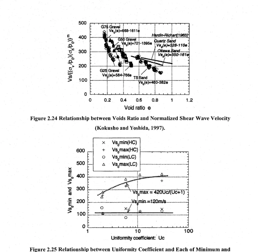
2.5.5 Kokusho and Yoshida (1997)... 45
2.5.6 Results o f som e Previous S tudies... 48
2 .6 C o r r e l a t i o n s b e tw e e n Vs o r G0 a n d S o i l P a r a m e t e r s ... ... 4 8 2.6.1 Lade and Nelson (1987)... 49
2.6.2 Bellotti et al. (1997)... 49
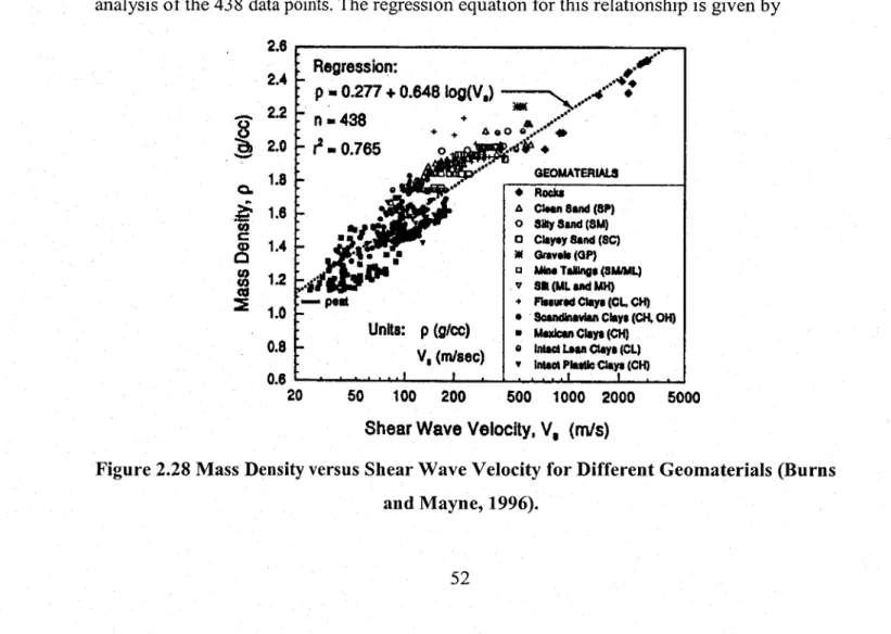
2.6.3 Burns and M ayne (1 9 9 6 )... 52
2.6.4 Mayne, Schneider and M artin (1999)... 54
2.6.5 Mayne (2001)... 54
2.1 C o m p a c t i o n o f S o i l a n d S h e a r M o d u l u s ... 55
2 .8 Co n c l u s i o n s ... 6 6 CHAPTER 3 NUMERICAL SIMULATIONS AND ANALYTICAL MODELS FOR PULSE VELOCITY T E ST S... 67 3.1 In t r o d u c t i o n... 6 7 3 .2 Fu n d a m e n t a l Co n c e p t sin Nu m e r ic a l Si m u l a t io n s... 67 3 .3 Nu m e r ic a l Sim u l a t io no f El a s t ic Wa v e s Tr a n s m is s io n t h r o u g h La b o r a t o r y Sp e c im e n s b y Be n d e r El e m e n t s ... 7 0 3.3.1 Introduction ... 70
3.3.2 Bender Element M odels... 71
3.3.2.1 Signals Interpretation in Tim e D o m a in ... 72
3.3.2.2 Cross-Correlation M eth o d ... 76
3.3.2.3 New Interpretation Method (Energy R is e ) ... 78
3.3.2.4 Shape of Output Signal and Sam ple’s H eight... 80
3.3.3 Conclusions...i... 82
3 .4 Ne w Mo d e so f Sh e a r in g Ex c it a t io n f o r Pu l s e Ve l o c it y Te s t s... 83
3.4.1 The Numerical M o d e l... 83
3.4.2 Excitation with 2mm-Diameter R adial S hearing... 84
3.4.3 Excitation with 26mm-Diameter Radial S hearing ... 87
3.4.4 All Base Radial Shear Excitation... 92
3.4.5 All Base Simple Shear Excitation... 95
3.4.6 The Best M ode o f E xcitation... 96
3 .5 Re f l e c t e d Wa v e sa n d Ne a r-Fie l d Ef f e c tin Pie z o e l e c t r ic Pu l s e Te s t s... 9 7 3.5.1 Introduction... 97
3.5.2 Numerical Simulations fo r Studying Near-Field Phenom enon... 97
3.5.3 A nalytical M odels fo r Studying the E ffect o f Sam ple D im ensions ... 112
3.5.4 Application o f Previous Equations to Labor a to iy T ests... 118
3 .6 Su m m a r y... 119
CHAPTER 4 DISPERSIVITY AND INTERPRETATION OF PULSE VELOCITY TESTS... 121 4.1 In t r o d u c t io n... 121 4 .2 A Ne w Cr it e r io nfor As s e s s in gt h e Sh e a r Wa v e Ar r iv a l Tim e in Ti m e Do m a i n... 121 4 .3 A Ne w In t e r p r e t a t io n Me t h o d f o r Pu l s e Te s t s ( Wig n e r-Vil l e En e r g y An a l y s is) ...122 4 .4 Ap p l ic a t io no f Wig n e r-Vil l e En e r g y An a l y s iso n Nu m e r ic a l Si m u l a t io n Re s u l t s... 126 4 .5 In t e g r a t in g t h e Gr o u p Ve l o c it y Cu r v ef o r Ob t a in in gt h e Ch a r a c t e r is t ic Ve l o c i t y... 130 4 .6 Co n c l u s i o n s... 133
CHAPTER 5 DEVELOPMENT OF A NEW PIEZOELECTRIC DEVICE FOR
PULSE VELOCITY TESTS: RING ACTUATORS SETUP...135
5.1 In t r o d u c t io n... 135 5 .2 Pie z o e l e c t r ic Rin g-Ac t u a t o r sa n dt h e ir Pr e f e r e n c e ... 135 5.3 Ma n u f a c t u r in g t h e Rin g Ac t u a t o r s Se t u p ...138 5.4 St r a in sin Ring Ac t u a t o r s ... 144 5 .5 Te s t e d So il s... 148 5.6 Th e Us e d La b o r a t o r y Se t u p s ... 149 5 .7 De v e l o p m e n to ft h e Ring Ac t u a t o r s Se t u p... 150 5.7.1 Setup 1 ... 150 5.7.2 Setup 2 ... 156 5.7.3 Setup 3 ... 167 5.7.4 Setup 4 ... 170 5.7.5 Setup 5 ... 174 5.7.6 Setup 6 ... 179 5.7.7 Setup 7 ... 184 5.7.8 Setup 8 ... 18 8 . 5 .8 Op t im iz in gt h e Pe r ip h e r a l El e c t r o n ic Eq u i p m e n t s...191 5 .9 Ac c u r a c ya n d Tim e De l a yo ft h e Ne w Se t u p... ... 195 5 .1 0 Co n c l u s i o n s... 198
CHAPTER 6 EXPERIMENTAL TESTS AND RESULTS ... 199
6.1 In t r o d u c t io n... 199
6.2 Ef f e c to f In p u t Wa v e Sh a p e... 199
6.3 Te s t sin Oe d o m e t e r Ringa n d Pl e x ig l a s s Mo l d s... 2 0 4 6.4 So il Co m p a c t io na n d Sh e a r Wa v e Ve l o c i t y...221
6 .5 Su m m a r y... 231
CHAPTER 7 CORRELATING SHEAR WAVE VELOCITY TO IN SITU TESTS INDICES AT PERIBONKA D A M ... 233
7.1 In t r o d u c t io n...2 33 7 .2 Sit e De s c r ip t io n... 2 33 7.3 Th e Fill Soila n dits La b o r a t o r y Te s t s ...2 3 4 7 .4 Th e Da t a Ba s ef o rt h e Co r r e l a t i o n s... 2 3 7 7 .5 Tr e a t m e n to f Te s t Da t a... 2 3 9 7 .6 Vo id s Ratioa n d Sh e a r Wa v e Ve l o c it y f o r Dif f e r e n t So il Gr a d i a t i o n s ... 2 5 4 7 .7 Co r r e l a t in g K, t o Pe n e t r a t io n Te s t s In d i c e s... 2 5 6 7.7.1 Relationship between VS] and qcl... 256
7.7.2 Relationship between Vs] and (Nj)6o... 264
7 .8 Co n c l u s io n s ...265
CHAPTER 8 CONCLUSION AND RECOMMENDATIONS... 267
8.1 In t r o d u c t io n...2 6 7 8.2 Ou t p u to fth e St u d y... 2 68 8.3 Co n c l u s io n sa n d Re c o m m e n d a t i o n s ... 2 7 0 8 .4 Re c o m m e n d a t io n sf o r Bu il d in g Rin g Ac t u a t o r s Se t u p... 2 7 4 8.5 Fu r t h e r Re s e a r c h... 2 75 REFERENCES ... 277
APPENDIX A CORRELATIONS BETWEEN SHEAR WAVE VELOCITY (OR ELASTIC SHEAR MODULUS) AND IN SITU TESTS INDICES ... Al
A . l Fvo r G0Co r r e l a t i o n s t o S P T In d e x... . ... A 2
A .I.I Ohta and Goto (1978)... ...A2
A .1.2 Im ai and Tonouchi (1 9 8 2 )... A3 A .1.3 Im ai and Yokota (1 9 8 2 )... ,...A9 A.1.4 Seed, Idriss a n d Arango (1 9 8 3 )... A9 A.1.5 Other C orrelations... A9
A.2CORRELATIONS BETWEEN F ^O R G0 AND C P T IN D E X ...A14
A.2.1 B a ld ie ta l. (1986)....,... A14 A.2.2 Baldi et al. (1 9 8 9 )... A14 A.2.3 Rix and Stokoe (1991)... ...A 16 A.2.4 Hegazy and M ayne (1995)... A 16 A.2:5 Kokusho and Yoshida (1997)... A 17 A.2.6 Simonini and Cola (2000)... A18 A.2.7 Jam iolkowski et al. (2004)...A 19 A.2.8 Other S tu d ie s ... A 19
A.3CONCLUSION S ... A 2 3
APPENDIX B CORRELATIONS FOR ESTIMATING RELATIVE DENSITY OF
SOIL FROM PENETRATION TEST INDICES...Bl
B . l CORRELATIONS FOR ESTIMATING RELA TIV E DENSITY FROM S P T ...B 2
B.1.1 M eyerhof (1 9 5 7 )... B2 B .l.2 Gibbs and H oltz (1957)...B2
B. 1.3 Peck and Bazaraa (1969)... B2
B .l.4 Bieganousky andM arcuson (1976)...B3 B. 1.5 Kokusho et al. (1983).,... B3 B .l.6 Tokimatsu a n d Yoshimi (1983) ...B3 B .l.7 Skempton (1 9 8 6 )...B4 B .l.8 Cubrinovski a n d Ish ih a ra (1999)... B4 B .l.9 Hatanaka and F eng (2006)... B5
B .2Co r r e l a t i o n s f o r Es t i m a t i n g Re l a t i v e De n s i t y f r o m C P T ... . ... B 8
B.2.1 Jamiolkowski et al. (1985)... B8 B.2.2 B a ld ie ta l. (1986)... B9 B.2.3 Tanizawa et al. (1 9 9 0 )... B9 B.2.4 Jamiolkowski et al. (2 0 0 1 )... B9
APPENDIX C SCREEN DISPLAY FROM THE PULSE TEST INTERPRETATION
SOFTWARE FOR SOME CARRIED OUT RING ACTUATORS
TESTS ... Cl
L IS T O F T A B L E S
Table 2.1 Damping Ratio and Input Frequency Effect on the Error o f Travel Time Using Cross-Correlation
Method (Santamarina and Farn, 1995)... 30
Table 2.2 Stiffness Coefficients o f Dry Washed Mortar sand from Seismic Body Waves (Stokoe, 1991)...44
Table 3.1 The Carried out Numerical Simulations for Bender Elements Pulse Test... 72
Table 3.2 Numerical Simulations for the New Modes o f Shearing Excitation... 84
Table 3.3 Numerical Simulations for Studying Near-Field Effect... 103
Table 3.4 Typical Values o f Elastic Modulus and Poisson’s Ratio (Das, 1994)... 116
Table 5.1 Properties o f the Used Piezoelectric Material (850-E)... 139
Table 5.2 Dimensions and Properties o f the Chosen Piezoelectric Cylinders (850-E)... 145
Table 5.3 Computed Strains o f Unrestrained Piezoelectric Cylinders/Rings... 146
Table 5.4 Rough Estimation o f Deformations for Unrestrained Piezoelectric Rings... 147
Table 5.5 Grain Size Characteristics o f some Soil Types... 149
Table 5.6 Dimensions o f the Used Laboratory Setups... 150
Table 5.7 Specifications o f the Ring Actuator Setups Manufactured in this Study... 154
Table 5.8 Frequency Constant o f the Used Piezoelectric Material... 177
Table 5.9 Resonant Frequency Factor for Different Materials...180
Table 5.10 Density and Elastic Waves Velocity o f Three Materials... 195
Table 6.1 The Carried out Tests in the Large Oedometer Ring and in Plexiglass M olds...204
Table 6.2 The Carried out Ring Actuators Pulse Tests on Compacted Soils... 222
Table 7.1 Before-Compaction CPT within 10-m from the MASW Lines...243
Table 7.2 CPT and MASW Data Base at Peribonka Dam... 248 Table A .l Vs Empirical Equations in Four Characteristic Indexes (Ohta & Goto, 1978)... A4 Table A .2 Correlations for Estimating Shear Wave Velocity from SPT Number... A l 1
Table A.3 Existing Correlations for Estimating Shear Wave Velocity from Cone Penetration Test Results A20
Table B .l Corrections o fN According to Fines Content... B4 Table B.2 Correlations for Estimating Relative Density from SPT N-Value...B6 Table B.3 Correlations for Estimating Relative Density from Cone Penetration Test Results... B10
L IS T O F F IG U R E S
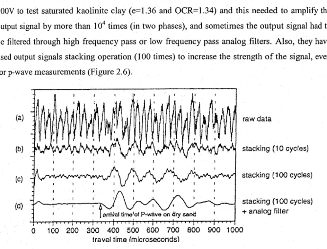
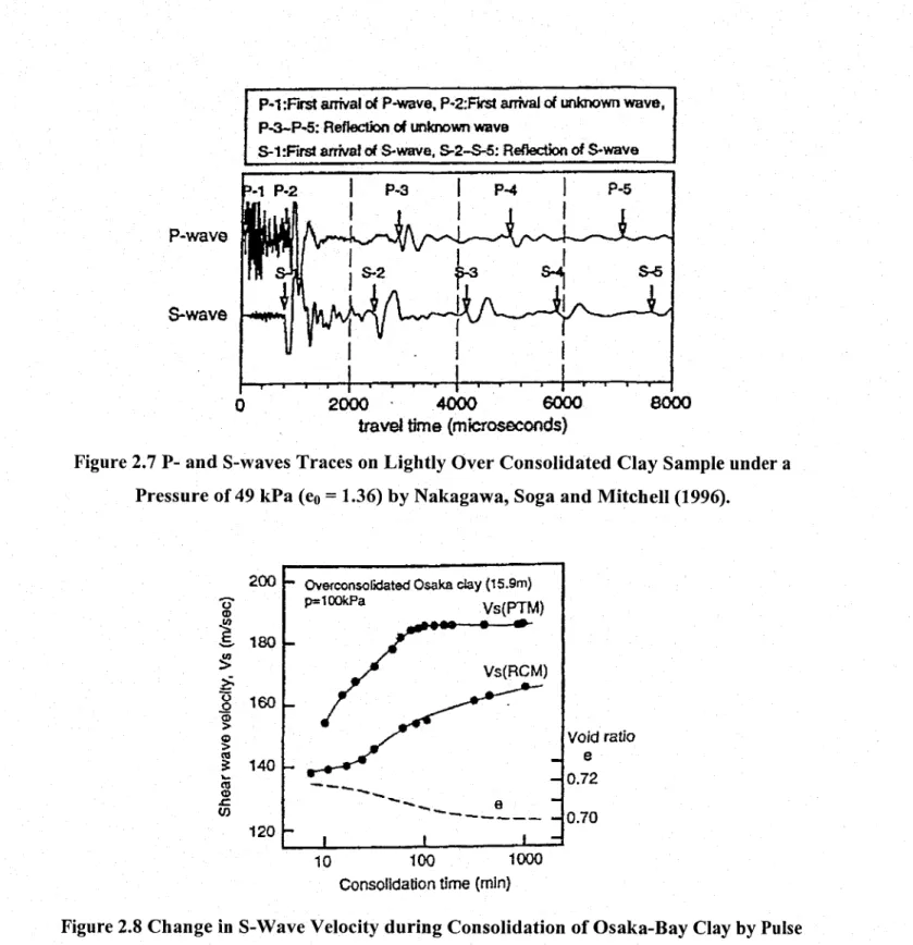
Figure 2.1 The Phase Response o f a Piezo-Actuator System... 9 Figure 2.2 Wiring, Polarization and Displacement Details o f Compression (a), Bender (b) and Shear-Plate (c) Transducers (after Brignoli, Goti and Stokoe II, 1996)... 13 Figure 2.3 Shear-Plate and Compression Transducers by University o f Western Australia (Ismail & Rammah, 2005) and a Commercial Shear Plate Setup...13 Figure 2.4 Two Sizes o f Shear Plate Transducers (Commercial and UWA Plates)... 14 Figure 2.5 Shear-Plates for Torsional Pulse Test in a Triaxial Setup (Nakagawa, Soga and Mitchell (1996)... 14 Figure 2.6 Effect o f Stacking and Analog Filtering on Wave Signal Forms; Fine Sand Sample under ct'c = 39.2 kPa (Nakagawa, Soga and Mitchell, 1996)... 15 Figure 2.7 P- and S-waves Traces on Lightly Over Consolidated Clay Sample under a Pressure o f 49 kPa (e0 =
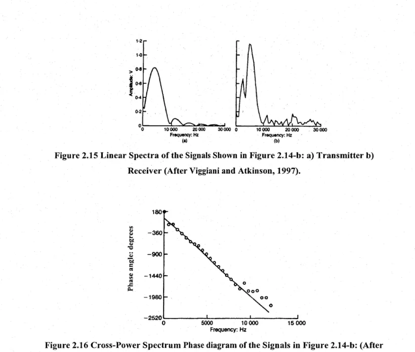
1.36) by Nakagawa, Soga and Mitchell (1996)... 16 Figure 2.8 Change in S-Wave Velocity during Consolidation o f Osaka-Bay Clay by Pulse Transmission and Resonant Column (Nakagawa, Soga and Mitchell, 1996)... 16 Figure 2.9 Typical Bender Elements Wiring, Polarization and Displacement Details: a) Transmitter; b) Receiver (Lings and Greening, 2001)... 17 Figure 2.10 Bender Elements Setup in a Triaxial Cell (Nakagawa et al., 1997)... 18 Figure 2.11 Very Large Electromagnetic Interference Masks the Arrival o f the Mechanical Wave (Tanner, 2004). ... 19 Figure 2.12 Typical Bender/Extender Elements Wiring, Polarization and Displacement Details: a) Transmitter; b) Receiver (Lings and Greening, 2001)... 19 Figure 2.13 Voltage Variation at Receiver for Step-Input Excitation [After: a) Jovicic, Coop and Simic (1996), b) Arulnathan, Boulanger & Riemer (1998) and c) Viggiani and Atkinson (1997)]...23 Figure 2.14 Bender Element test Results: input and output signals [After: a) Arulnathan, Boulanger and Riemer (1998) and b) Viggiani and Atkinson (1997)]... 24 Figure 2.15 Linear Spectra o f the Signals Shown in Figure 2.14-b: a) Transmitter b) Receiver (After Viggiani and Atkinson, 1997)... 26 Figure 2.16 Cross-Power Spectrum Phase diagram o f the Signals in Figure 2.14-b: (After Viggiani and Atkinson,
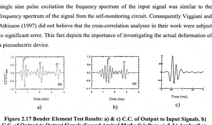
1997)... 26 Figure 2.17 Bender Element Test Results: a) & c) C.C. o f Output to Input Signals, b) C.C. o f Output to Output Signals (Second Arrival Method) [after: a) & b) Arulnathan, Boulanger and Riemer (1998), c) Viggiani and Atkinson (1997)]... 27 Figure 2.18 Cross-power Spectra o f the Signals Shown in Figure 2.14-b (After Viggiani and Atkinson, 1997).. 28 Figure 2.19 Cancelling the Near Field Effect with a Distorted Input W ave... 35 Figure 2.20 Dispersion Curve for Transmitter-Receiver Spacing o f 75-mm (Blewett et al., 2000)... 38 Figure 2.21 Deformation o f a Piezoelectric Ring Using Four-Node Tetrahedron Mesh (Peelamedu et al., 2003).40 Figure 2.22 Shear Modulus Number MG versus Void Ratio for Different Types o f Soils (Jamiolkowski, Leroueil and Lo Presti, 1991)... 43 Figure 2.23 Grain Size Distribution o f Five Types o f Soils Tested by Kokusho and Yoshida (1997)...46 Figure 2.24 Relationship between Voids Ratio and Normalized Shear Wave Velocity (Kokusho and Yoshida, 1997)... 47 Figure 2.25 Relationship between Uniformity Coefficient and Each o f Minimum and Maximum Normalized Shear Wave Velocity (Kokusho and Yoshida, 1997)...47 Figure 2.26 Shear Modulus as a Function o f Relative Density for Toyoura Sand (Bellotti et al., 1997)... 51
Figure 2.27 The versus Dr for Normally and Over-Consolidated Toyoura Sand (Bellotti et al., 1997)... 51
Figure 2.28 Mass Density versus Shear Wave Velocity for Different Geomaterials (Burns and Mayne, 1996)... 52 Figure 2.29 Multiple Regression Evaluation o f Total Unit Weight for Different Geomaterials (Bums and Mayne,
1996)... 53 Figure 2.30 Relationship between Mass Density, Shear Wave Velocity and Depth o f Overburden for
Geomaterials (Mayne, Schneider and Martin, 1999)... 54 Figure 2.31 Stages o f Unsaturated Conditions and Related Phenomena (Santamarina, Klein and Fam, 2001).... 57 Figure 2.32 Details o f a Seismic Compaction Mold (Ismail and Rammah, 2006)... 58 Figure 2.33 A Photo o f the Shear Transducer with the Rotation Mechanism (Ismail and Rammah, 2006)... 58 Figure 2.34 Determination o f Arrival Time from Three Frequency Traces (Ismail and Rammah, 2006)... 59
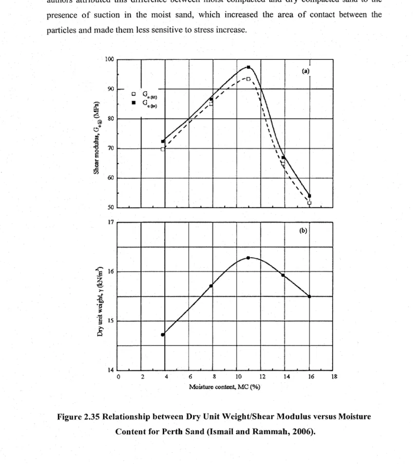
Figure 2.35 Relationship between Dry Unit Weight/Shear Modulus versus Moisture Content for Perth Sand
(Ismail and Rammah, 2006)... 60
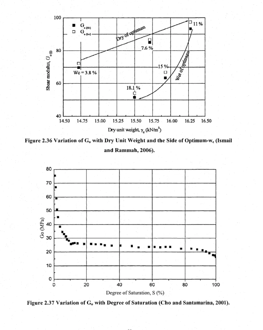
Figure 2.36 Variation o f G0 with Dry Unit Weight and the Side o f Optimum-wc (Ismail and Rammah, 2006)... 61
Figure 2.37 Variation o f G0 with Degree o f Saturation (Cho and Santamarina, 2001)... 61
Figure 2.38 Influence o f Degree o f Saturation on (G0)|1V o f Perth Sand (initial yd = 16 kN/rn3) during Isotropic Compression Test, (Ismail and Rammah, 2006)... 62
Figure 2.39 Variation o f (G0),j with Vertical Stress for Compacted Moist Sand (Ismail and Rammah, 2006)... 62
Figure 2.40 Variation o f V, with Compaction Water Content and Isotropic Confining Pressure (Claria Jr. and Rinaldi, 2007)... 63
Figure 2.41 Variation Vs with crm and wc: a) Samples Compacted Dry o f Optimum (Md), b) Samples Compacted Dry o f Optimum (Md'), c) Samples Compacted at the Optimum, d) Samples Compacted Wet o f Optimum (Mw) [Claria Jr. and Rinaldi, 2007]...64
Figure 2.42 Variation o f Vs with am for Samples Compacted at Different Moisture Contents but Tested at a Similar Degree o f Saturation (Clarih Jr. and Rinaldi, 2007)... 65
Figure 3.1 Rayleigh Damping versus Frequency (FLAC® Manual)... 70
Figure 3.2 A Model for a Bender Element Setup Installed in a Triaxial Apparatus... 73
Figure 3.3 Output Signals o f the Numerical Simulations for Bender Elements Pulse Test (Groups 1 & 2 )...74
Figure 3.4 Variation o f Direct Arrival Time with Input Frequency for points A, B and C Using Results of Simulations 1 and 2 ... 75
Figure 3.5 Cross-Correlation Arrival Times o f Shear Wave for Results o f Simulations No. 1 and No. 2 ...76
Figure 3.6 Cross-Correlation Based on both Input Force and Deformation at Emitter for Results o f Simulations 1 and 2 ... 77
Figure 3.7 Input and Output Signals, their C.C Function and its Energy Envelope for Simulation No. 1 (Fr = 12.5 kHz)... 78
Figure 3.8 The Energy Envelop and C.C. Function for a Simulation o f Group No. 2 ... 79
Figure 3.9 Different Arrival Times for Results o f Simulations 1 and 2 ...80
Figure 3.10 Output Signals o f the Numerical Simulations for Bender Elements Pulse Test (Groups 3 and 4 )...81
Figure 3.11 The Numerical Model and its Boundary Conditions... 83
Figure 3.12 Output Signals o f Simulation Group No. 5 (Excitation Area o f 2-mm-Diameter)... 85
Figure 3.13 Displacement Vectors for Simulation 5 at Different Times... 86
Figure 3.14 Lateral Displacements at Receiver for Simulation 6 ...88
Figure 3.15 Vertical Displacements at Receiver for Simulation 6 (Fr=30 kHz)...89
Figure 3.16 Lateral Displacement at a Different Reception Point for Simulation 6... 90
Figure 3.17 Lateral Displacements at Receiver for Simulation 7 ...91
Figure 3.18 Displacement Vectors for Simulation 7 at Two Times (Fr = 30 kHz)... 92
Figure 3.19 Lateral Displacements at the Receiver for Simulation 8 ... 93
Figure 3.20 Victor Displacements for Simulation 8 during Waves Travel through the Sample (Fr = 20 kHz) 93 Figure 3.21 The Travel Time using Different Methods for Simulation 8...94
Figure 3.22 Lateral Displacements at Receiver for Simulation 9 ... 95
Figure 3.23 The Elements Displacements in Simulation 9 while the S-wave is Halfway and at Receiver (Fr = 30 kHz)... 96
Figure 3.24 Displacement Vectors for Simulation N o .l (Fr. = 25 kHz)...99
Figure 3.25 Amplitude Decrease with Increasing Input Wave Frequency... 104
Figure 3.26 Displacement Vectors for Simulation No. IQ ...105
Figure 3.27 The Received Signals for Groups o f Simulations No. 1 and IQ ... 106
Figure 3.28 The Geometry o f the Used Model for Simulations 10, 11 & 12 (the mesh o f the model is 0.5mm squares)... 109
Figure 3.29 Output Signals for Group o f Simulation No. 10 at Different Damping Ratios and Boundary Conditions... 110
Figure 3.30 Output Signals for Group o f Simulation No. 11 at Different Input Frequencies and Damping Ratios. ...I l l Figure 3.31 Results o f Simulation Group No. 12 at Different Input Frequencies...112
Figure 3.32 The Critical Path o f a Reflected Compression Wave in an Oedometer Cell with Bender Elements Setup...113
Figure 3.33 Reflected P-wave Arrival Time with Respect to S-wave Arrival versus Poisson's Ratio in Triaxial Cells with Bender-Elements Setup... 114
Figure 3.34 Reflected P-wave Arrival Time with Respect to S-wave Arrival versus Poisson's Ratio in some
Oedometer Cells with Bender-Elements Setup... 115
Figure 3.35 Direct and Side-Reflected Paths in an Oedometer Cell (Dim. in mm)... 116
Figure 3.36 P-wave Arrival Times with Respect to S-wave Arrival versus Poisson's Ratio in a Large Oedometer Cell for a Pulse Test by Disks Setup...117
Figure 3.37 Direct and Side-Reflected Paths in a Proctor Mold...117
Figure 3.38 P-wave Arrival Times with Respect to S-wave Arrival versus Poisson's Ratio in Proctor Mold during a Pulse Test by Disks Setup... 118
Figure 3.39 Pulse Test on an Ottawa Sand Sample in the Large Oedometer Cell that Proves the Reflection at Sides... 119
Figure 4.1 Wigner-Ville Energy Analysis for a Numerical Simulation Result...124
Figure 4.2 Wigner-Ville Energy Analysis for a Laboratory Pulse Test on Ottawa Sand...125
Figure 4.3 Analyses o f some Numerical Simulations in the Frequency Domain Using Wigner-Ville Technique. ...127
Figure 4.4 Numerical Simulation o f a Pulse Test Using Ring Actuators Interpreted by Wigner-Ville Energy Analysis Method... 128
Figure 4.5 Simulation 11(a) Interpreted by Wigner-Ville Energy Analysis...129
Figure 4.6 Output Signals for Group o f Simulations No. 13...132
Figure 4.7 Integration o f Vgr for Obtaining the Characteristic Vs for Simulation No. 13 (Fr = 20 kHz)...133
Figure 5.1 Interference o f Waves at Receiver Due to Reflections on Pedestal and Top Cap for a Bender-Elements System... 136
Figure 5.2 Dimensions and Deformations o f a Piezoelectric Ring Actuator Polarized in the Radial Direction.. 137
Figure 5.3 Bender Element Mode o f Excitation... 138
Figure 5.4 The Configurations o f Piezoelectric Cylinders... 140
Figure 5.5 Dimensions o f the Chosen Piezoelectric Tubes for Having Rings... 141
Figure 5.6 Piezoceramic Ring and Cylinder Transducers with Schismatic Drawing for their Composition 141 Figure 5.7 Manufacturing a Piezoelectric Ring Setup...142
Figure 5.8 A Ring Actuator Glued to Porous Stone...143
Figure 5.9 Grain Size Distribution o f Ottawa Sand (C-109)...148
Figure 5.10 The Grain Size Distribution Curves for some Soil Types... 149
Figure 5.11 A Design for Cap Equipped with a Ring Actuator for Carrying out Pulse Tests at Laboratory (Setup 1)... 151
Figure 5.12: Small-Size Piezoelectric Rings and Porous Stones... 151
Figure 5.13 The First Setup that Incorporated Ring Actuators for Pulse Testing o f Soil: Emitter & Receiver Units... 152
Figure 5.14 Pulse Test Equipments and Wiring, Connected to an Oedometric Sample Loaded by a Simple Frame. ... 152
Figure 5.15 Design Drawings o f the Ring Actuators Setup for Measuring V p and V s in an Oedometric Ring (Setup 2)... 156
Figure 5.16 A Piezoelectric Ring Actuators Setup for Measuring Shear Wave Velocity o f Soil in a Proctor Mold (Setup 2 )... 157
Figure 5.17 Large Oedometer Cell with Piezoelectric Ring Actuators (Setup 2)... 158
Figure 5.18 Transmitter o f Setup 2 after Connecting the Grounding Wire... 159
Figure 5.19 Ring Actuator Pulse Tests in an Oedometer Ring (Setup A) and in a Proctor Mold (Setup B) during One Dimensional Compression Tests... 159
Figure 5.20 LG4 Till Proctor Sample Tested by Setup 2 Using a Rectangular Input Signal (t=30ps)... 160
Figure 5.21 Proctor Sample o f a LG4 Till Tested by Setup 2 Using a Rectangular Input Signal (t=15ps)... 162
Figure 5.22 LG4 Proctor Sample Tested by Setup 2 Using Sine Wave o f 20 kHz... 163
Figure 5.23 Coupling o f Compression and Shear Waves on Output Signal in a Pulse Test on Medium-Density Milby Sand Sample Tested by Setup 2 in an Oedometer Cell... 164
Figure 5.24 Pulse Test on Milby Sand Sample in Large Oedometer Cell...165
Figure 5.25 Proctor Sample o f Milby Sand (wc = 6.0 %, a v = 11.63 kPa) Tested with Setup 2 ...166
Figure 5.26 Drawing for Setup 3 in an Oedometeric Ring and a Picture for it Showing the Emitter and Receiver Units... 168
Figure 5.27 Milby Sand Proctor Sample Tested by Setup 3 Using Half-Sine Input (Fr = 12.5 kHz)...169
Figure 5.29 The Emitter Unit o f Setup 4 ... 171
Figure 5.30 Steps o f Manufacturing Setup 4 in Photos... 172
Figure 5.31 Pulse Test on Proctor Sample o f Concrete Sand Using Setup 4 ... 173
Figure 5.32 Pulse Test on Milby Sand by Setup 4 in Large Oedometer Cell...174
Figure 5.33 Effective Mass and Displacement o f a Piezo-Actuator (after PI Co.)... 175
Figure 5.34 The Emitter Unit o f Setup 5...177
Figure 5.35 Pulse Test on Proctor Sample o f Concrete Sand Using Setup 5... 178
Figure 5.36 Pulse Test on Proctor Sample o f LG4 Using Setup 5 ... 179
Figure 5.37 Pulse Test on Proctor Sample o f Concrete Sand Using Setup 5 (Fr=8 kHz)...180
Figure 5.38 Setup 6 and its Modifications... 181
Figure 5.39 Pulse Test on Fine Ottawa Sand in a Large Oedometric Ring... 182
Figure 5.40 Pulse Test on Fine Ottawa Sand in a Large Oedometric Ring (L=17.65mm)...183
Figure 5.41 Pulse Test on Fine Ottawa Sand in a Large Oedometric Ring (Pr. =116 kPa)...183
Figure 5.42 A Ring Setup with Solid Interior Stone and its Deformation Profile...184
Figure 5.43 A Ring Setup with Divided Interior Stone and its Deformation Profile...185
Figure 5.44 Some Photos for Setup 7c and its Manufacturing Processes... 186
Figure 5.45 Effect o f Output Signal Trimming on C.C. Function and W.V. Analysis... 187
Figure 5.46 Trimming Effect on Dispersion Curves o f Phase and Group Velocities...188
Figure 5.47 A Very Thin Layer o f Silt at each Cap Enhances Interaction... 189
Figure 5.48 A Drawing for the Emitter Unit o f Setup 8...189
Figure 5.49 A Photo for Setup 8 (without the Outer Aluminum Disc); the Sand Grains Cover the Porous Stone and Hides the Cuts... 190
Figure 5.50 The Second Arrival o f S-Wave is Clearly Recorded Using Ring Actuators... 191
Figure 5.51 Very Clear Separation between P- & S-Waves when Testing Weak Samples... 192
Figure 5.52 The Used Power Amplifiers during this Study... 194
Figure 5.53 Calibration Results for the Ring Actuators Setup Using a Plexiglass Cylinder o f 68-mm-Length.. 196
Figure 5.54 Output Signals for Pulse Tests by Ring Actuators on a Plexiglass Cylinder o f 93.2-mm-Length... 196
Figure 5.55 Output Signals for Pulse Tests by Ring Actuators on a Plexiglass Cylinder o f 101.7-mm-Length. 197 Figure 5.56 Pulse Tests Result on Plexiglass Cylinders o f Variable Lengths...197
Figure 6.1 Pulse Test on Dry Ottawa Sand Sample in the Oedometer Cell...201
Figure 6.2 Ottawa Sand Sample Tested by Different Input Shapes; Test 48; Setup 8...201
Figure 6.3 Sine Input versus Versed-Sine Shapes for Pulse Tests; Setup 8 ...202
Figure 6.4: Sine Input versus Winged-Sine Shapes for Pulse Tests; Setup 8... 203
Figure 6.5 Stress-Strain Relationship for Loose Ottawa Sand (C-109); Test 4 7 ... 205
Figure 6.6 Variation o f Vs with Vertical Stress for Loose Ottawa Sand (C-109) (Setup 7, Test-47, Ls= 35.3mm, Dr = 30%, e = 0.69, yd = 1.57)... 206
Figure 6.7 Variation o f Vs with Average Stress for Loose Ottawa Sand (Test-47)... 206
Figure 6.8 Variation o f Vp with Vertical Stress for Loose Ottawa Sand (C-109); Test 4 7 ... 207
Figure 6.9 Relationship between Vp and Vertical Stress for Loose Ottawa Sand (C-109); Test 4 7 ... 208
Figure 6.10 Relationship between Vs and Vertical Pressure for Loose Ottawa Sand (C-109); Test 47... 208
Figure 6.11 Relationship between V sl and Voids Ratio for Loose Ottawa Sand (C-109); Test 4 7 ...209
Figure 6.12 Relationship between Vsl and Voids Ratio for Loose Ottawa Sand (C-109); Test 4 7 ...210
Figure 6.13 Relationship between Poisson’s Ratio and Vertical Pressure for Loose Ottawa Sand (C-109); Test 47. 210 Figure 6.14 Ottawa Sand (C-109) (Test-46, Setup 8, Ls = 95mm, Dr = 83%, e = 0.53, yd = 1.73 t/m3) ... 211
Figure 6.15 Normalized Vs for Ottawa Sand (C-109) (Test-46, Ls= 95mm, Dr = 83%, e = 0.53, yd = 1.73)...212
Figure 6.16 Variation o f Vs with Voids Ratio for Ottawa Sand (C-109) (Test-46, Ls= 95mm, Dr = 83%, e = 0.53, yd= 1-73)... 213
Figure 6.17 VsI versus Voids Ratio for Ottawa Sand (Test-46, Ls= 95mm, Dr = 83%, e = 0.53, yd = 1.73)... 213
Figure 6.18 The Deformation Curve o f Milby Sand in an Oedometer Ring (Test 3 )... 214
Figure 6.19 Repeated Test Using Setup 4 for a Dry Milby Sand Sample in Oedometer Cell Showing the Variation o f Vs with Vertical Stress (Test 3)... 215
Figure 6.20 Variation o f Vp with Vertical Stress for Milby Sand in Oedometer Cell... 216
Figure 6.21 Variation o f Vs with crv0'25 for Milby Sand (Test 3)... 216
Figure 6.23 Relationship between Elastic Modulus and Voids ratio for Ottawa Sand (Test No. 3 )... 217
Figure 6.24 Variation o f Vs with Vertical Pressure for Dense Ottawa Sand in Test 4 0 ...218
Figure 6.25 Variation o f Vs with Voids Ratio in Test 4 0 ... 219
Figure 6.26 One-Dimensional Deformation Curves for Tests 46 and 4 0 ... 220
Figure 6.27 Relationship between VsI and Voids Ratio for Results o f Test 4 0 ... 220
Figure 6.28 Relationship between Average Stress Normalized Vs and Voids Ratio for Results o f Test 4 0 ... 221
Figure 6.29 Stress-Strain Relationships for LG4 Till in Tests 49, 43 & 42... 223
Figure 6.30 Relationships between Vs and Vertical Pressure for LG4 Till Samples... 223
Figure 6.31 Variation o f Vs! with Vertical Pressure for Proctor Samples o f LG4 Till (Tests 42, 43 and 49)... 224
Figure 6.32 Variation o f Vsl with Voids Ratio for LG4 Till Proctor Samples in Tests 42, 43 and 4 9 ... 224
Figure 6.33 Standard Proctor Compaction Curves for LG4 Till...225
Figure 6.34 Vs - Compaction Curve for LG4 Till at Three Different Pressures... 226
Figure 6.35 Elastic Shear Modulus o f Compacted LG4 T ill...227
Figure 6.36 Vs versus Applied Pressure for Compacted LG4 Till Samples... 228
Figure 6.37 Variation o f Vs with Voids Ratio for LG4 Till Samples under Different Pressures... 228
Figure 6.38 Variation o f VsI with Water Content for LG4 Till Samples in Proctor Mold... 229
Figure 6.39 Standard Proctor Test for Concrete Sand... 230
Figure 6.40 Shearing Rings Test on the Concrete Sand in Proctor Mold...230
Figure 7.1 The Different Sections o f the Dam (after Hydro-Quebec)... 234
Figure 7.2 Grading o f the Fill Materials...235
Figure 7.3 The Maximum and Minimum Densities o f the Fill Materials...235
Figure 7.4 The Maximum and Minimum Voids Ratio o f the Fill Materials...236
Figure 7.5 Variation o f Saturated Density with Soil Type...236
Figure 7.6 Variation o f emax and emin with Uniformity Coefficient... 237
Figure 7.7 Variation o f emax and e,™, with Coefficient o f Curvature...238
Figure 7.8 Variation o f emax and eniin with D 50... 238
Figure 7.9 Locations o f MASW Lines at Peribonka Dam Site... 239
Figure 7.10 Locations o f the Field Tests, Boreholes and U-Geophysical Survey Lines...240
Figure 7.11 Geologic Cross Section at Lines 1 and 2 ... 241
Figure 7.12 Geologic Cross Section at Lines 3 and 4 ...242
Figure 7.13 V sl and qclN Profiles (CPT 227 & CPT 228)...244
Figure 7.14 V sl and qclN Profiles (CPT 54 & CPT 55)... 245
Figure 7.15 V sl and qclN Profiles (CPT 62 & CPT 169)... 246
Figure 7.16 V sl and qclN Profiles (CPT 86 & CPT 177)... 247
Figure 7.17 Estimation o f D r and Vs Based on CPT Results, and the Measured C-Profile by M ASW ...250
Figure 7.18 a) Profiles o f V sl & qclN at Location o f CPT-55, b) Estimated Relative Density based on SPT 251 Figure 7.19 Test Results and Estimation o f Friction Ratio (Rf) and Material Index (Ic) for CPT-55... 252
Figure 7.20 Calculation o f OCR, Ko and Voids Ratio (e) Based on CPT and Vs Profiles...253
Figure 7.21 Different Voids Ratio Functions...255
Figure 7.22 Estimating Voids Ratio from Vsl for Different Soil Types... 255
Figure 7.23 A ll VS| - qciN Points o f Peribonka Dam Data Base...258
Figure 7.24 The Data Points in the Fill Soil...259
Figure 7.25 Data Points in the Fill Soil Excluding Abnormal Values... 260
Figure 7.26 The Relationship between Vsi and qciN for the Fill Soil (abnormal qc values corrected)... 261
Figure 7.27 Comparison between the Obtained Results in the Fill o f the Dam before Compaction and some Existing VsI - qc]N Correlations (Vs & qc Profiles are within 3.5m apart)... 262
Figure 7.28 Comparison between the Obtained Results in the Natural Soil before Compaction and some Existing V si - 9cin Correlations (Vs & qc profiles are within 3.5m apart)... 263
Figure 7.29 The Relationship between V s) and (N t)60for the Natural Soil...264
Figure 7.30 Comparison between the Obtained Results and the Existing VsI - (N , )60 Relationships... 265 Figure A .l Distribution o f Vs and Vp (lm ai and Tonouchi, 1982)... A5 Figure A.2 Relationships o f Vp and Vs to A Value (Imai and Tonouchi, 1982)... A6
Figure A.3 SPT N-Value versus Shear Wave Velocity for Different Soil Types (Imai and Tonouchi, 1982) A7
Figure A.4 Summarized Relationships o f Vs to N (Imai and Tonouchi, 1982)... A8 Figure A.5 Relationship between Dynamic Shear Modulus and SPT Blow Counts N (Imai and Tonouchi, 1982).
Figure A .6 Relationship between Small Strain Shear Modulus and SPT Number (Imai and Yokota, 1982)...A10 Figure A.7 Measured and Predicted Vs for Silica Sands (Baldi et al., 1989)... A15 Figure A.8 Relationship between Small Strain Shear Modulus and CPT Tip Resistance for Silica Sands (Baldi et al., 1989)... A15 Figure A.9 Normalized Shear Wave Velocity versus Normalized SPT N-Value (Kokusho and Yoshida, 1997).
... A18 Figure A.10 Gnuix to qc for Venice City Soil (Simonini and Cola, 2000)... A19
SY M B O L S A N D N O T A T IO N S
A SF age scaling factor for penetration-velocity equations
C piezo actuator capacitance
C.C cross-correlation function
Cc coefficient o f curvature
Q material constant in G a empirical equations
Cn overburden stress correction factor
Cp, c s
compressional and shear wave velocitiesCPT cone penetration test
Cu
coefficient o f uniformityD material damping ratio
D 5 0 median grain size
D io , D 3 0 , Deo grain size o f 10%, 30% and 40% passing, respectively
c h i strain coefficient (displacement normal to polarization direction)
d 3 3 strain coefficient (displacement in polarization direction)
D 0 , Di outer and inner diameter, respectively
D r relative density
E modulus o f elasticity (Young’s modulus)
e void ratio
<?i initial void ratio
e g constant in void ratio function
% ia x > C m in maximum and minimum void ratio
F cone friction ratio
FC fines content
F{e) void ratio function
f n J o resonant frequency
f F r frequency
f s measured cone sleeve friction
G shear modulus
g gravity acceleration (g = 9.81 m/s2) G max ; G 0 small-strain shear modulus
G s specific gravity
H height o f ring
I electrical current
Ic soil behavior type index
k
the wave-number1<33 ’ ^ 31 electromechanical coupling factors for a piezoelectric element
K soil bulk modulus
kf elastic frame bulk modulus
km mineral bulk modulus
kw interstitial pore-fluid bulk modulus K 0 coefficient o f earth pressures at rest
L , L S L b L« mi, m2 M, M max Mq , Mm , M e N N n n n, ng , na, nb N 60 ( Ni) 60 OCR P ' Pa Q Q Qm qc qciN r S, Sr *^opt. SPT T t Tc fs tp ,ref.
ut
pp gr Vp Vph Vpu yref. P VR Vs V s l , V s0 wc W compz
sample length bender lengthtip-to-tip distance in bender element test material constants for Vs empirical equation constrained modulus
modulus number
number o f wave-lengths (27i-count) measured blow count in SPT porosity
an exponent used in normalizing cone tip resistance an exponent o f stress in G0 / Vs empirical equations energy-corrected blow count
stress- and energy-corrected blow count overconsolidation ratio
mean effective pressure a reference stress o f 100 kPa material constant
dimensionless cone tip resistance
mechanical quality factor o f a piezoceramic measured cone tip resistance
normalized cone tip resistance radius o f ring actuator
degree o f saturation
maximum suction degree o f saturation standard penetration test
period o f a signal (1/Fr) time
curie point o f a piezoelectric element (°C) shear wave arrival time
compression wave arrival time
arrival time o f reflected compression wave measured cone pore pressure
peak-to-peak voltage volume
group velocity
compression wave velocity phase velocity
unconstrained compression wave velocity wave velocity o f reflected compression wave Rayleigh wave velocity
shear wave velocity
stress-normalized shear-wave velocity water content
compaction water content depth
y shear strain Y 3 If sat unit weight o f soil
Id dry unit weight o f soil
1 wavelength
% Lame’s constant
V Poisson’s ratio
S strain
friction angle
9 phase difference between two signals
m phase o f the cross-power spectrum
0 the phase angle (27iN)
p mass density
CO angular frequency
o'h horizontal effective pressure
t _ t
v m > ® o mean effective confining pressure _ f
Chapter 1
IN TR O D U C TIO N
1.1 Introduction
A soil specimen generally undergoes irreversible deformation under loading such that the stress-strain relations for loading and subsequent reloading are quite different from that for first loading. However, if a given cycle o f loading and unloading is repeated for a few cycles (about 10 to 20 cycles for sand and perhaps 100 or so for clay) the stress strain relation becomes a closed, long, narrow loop (hysteretic loop), whether the loading involves one dimensional strain, one-dimensional stress, or torsional loading (Hardin and Black, 1968). Two parameters have been used to define this stress-strain relation (hysteretic loop), namely; the vibration (dynamic) modulus and the damping. The modulus is defined by the slope o f a line from origin to the ends o f the loop, and the area of the loop is a measure o f the damping capacity o f the soil. These parameters determine the characteristics o f the corresponding (o f same amplitude) wave propagation, the modulus being related to the velocity o f propagation and the area o f the loop to the attenuation. For problems involving small-amplitude steady- state vibration, the soil can often be assumed to be linearly elastic if damping can be neglected, or viscoelastic. The assumption o f viscoelasticity should be a close approximation for all the small amplitude vibration problems.
The parameters defining the hysteretic loop stress-strain relation have been determined by measuring the force-displacement relation for a repeated loading test, such as cyclic torsional shear technique (ASTM 1987) or direct static stress-strain, or by the resonant- column technique. By the resonant-column technique the shear modulus (Gmax or G0) is determined from the resonant frequency o f a column of soil and the damping capacity can be determined from the amplitude o f vibration at resonance (Hardin, 1965) or by observation o f the decay o f free vibrations (Hall and Richard, 1963). Up till now, the damping capacity parameter has had little application. The most important soil param eter for the analysis o f small-amplitude soil vibration problems is the modulus. Recently, soil moduli at very small strains are being easily determined b y direct measurements o f shear wave velocity ( Vs) using piezoelectric transducers which can be mounted in many laboratory testing apparatuses. In the last two decades, different types o f transducers have been used including shear plate, bender
element, compression transducer, and bender/extender element. The m easurem ent simplicity, the immediacy o f the results and the possibility o f taking m easurements during other mechanical tests make this piezoelectric testing technique very attractive. Bender-elements method is the most com m only used technique for these measurements although o f its fundamental and interpretation problem s that were reported by m any researchers.
The piezoelectric pulse techniques have been used to measure the shear wave velocity o f soil since Lawrence (1963). These methods have gained limited practical application in geotechnical laboratories although w idely used. This is due to the perceived instrumental and interpretative problems. Identifying the exact time of arrival o f shear w ave is the m ost difficult and controversial part o f a pulse test. In extreme cases, the errors in G„mx values m ay be on the order o f 50% (Viggiani and A tkinson, 1995). The basic research into the area o f behaviour o f piezoelectric devices is far behind the effort put forth in the study o f soil behaviour using these sensors. Also, the study o f the interpretation problems o f piezoelectric pulse tests has been widespread, but no interpretation technique may claim preference. Bender-elements are the most commonly used devices for ^-measurements at laboratory. The determination o f
Gmax by resonant column m ethod is sophisticated and involved inputs o f the resonant
frequency o f the soil-equipment system, a variety o f device dependent calibration constants and specimen dimensions and mass. The resonant column test can be used to evaluate the stiffness o f soils at shearing strains ranging from 10"5 % to 1 %. However, analyses o f the test data are strictly valid only in the region o f very small strain (Isenhower, 1979) because analyses o f resonant column tests are based on the assumption that the behaviour o f soil is linear and elastic. Differences in shear modulus o f more than 50% may appear when comparing measurement results from the cross-hole test and the resonant column test for the same subsoil (Roesler, 1979). Piezoelectric devices can measure the shear modulus o f soil all over the strain range in a laboratory test; something behind the capability o f a resonant column test with a fraction o f its cost.
1.2 Importance of Shear Wave Velocity Measurements
For uncemented cohesionless soils, the shear-wave velocity (Vs) can be regarded as a fundamental engineering parameter. Vs can be an important tool in determining the physical properties o f soil because o f the direct relationship o f shear wave velocity o f soil to its physical properties. The m easurem ent o f the dynamic shear modulus is increasingly important
w ith regard to the investigation o f the dynamic properties o f the subsoil. The shear modulus at very small strains (Gmax or G0), which is directly related to shear wave velocity through soil bulk density,/?, {Gmnx = pVs ), is a key parameter in predicting soil behaviour and soil-structure interaction in many applications. The shear-wave velocity o f sand is also controlled primarily by the effective confining stresses and void ratio. Thus, there is an increasing interest in using shear-wave velocity to define the state of soil. The initial state o f a sand, defined by the void ratio and effective mean norm al stress relative to the steady/critical state at the same stress level, can be used to predict its large-strain response [Roscoe et al. (1958) and Been and Jefferies (1985)]. Robertson et al. (1992) suggested values o f normalized shear-wave velocity to evaluate the in-situ state o f cohesionless soils. They could identify the boundary between contractant or dilatant sands (loose or dense). The stiffness o f soil at very small strain, Gmax, is a useful parameter for characterizing the non-linear stress-strain behaviour o f soil for monotonic loading and it is required for analyses o f the dynamic and small strain cyclic loading o f soils.
The small-strain shear modulus of soil, G„wx, also termed elastic modulus, is a fundamental parameter in m any kinds of static and dynamic analyses involving deformational calculations (Richart et al., 1970), or liquefaction analysis. Recently, Gnwx is used in conventional static loading problems applications. For example, using the modulus degradation hyperbolas for degrading the elastic modulus to strain levels relevant to deformation problems in geotechnical engineering such as foundation settlement and determining the stress-strain-strength curves for soil (Burland, 1989; Tatsuoka and Shibuya, 1991, Bums and Mayne, 1996; Mayne et al. 1999). Gmax is also important in predicting soil behaviour during earthquakes, explosions, or machine and traffic vibrations. It can be equally important for small strain cyclic situations such as those caused by wind or wave loading. Knowledge o f the dynamic shear modulus is necessary for the design o f vibration isolation measures. Gmax may also be used as an indirect indication o f various soil parameters as it usually correlates well to other soil properties such as density, fabric, and liquefaction potential. It m ay also be used to indicate sample disturbance by comparing laboratory and field measurements. Besides providing information about the dynamic characteristics o f soil, measurements o f Vp and Vs w ith piezoelectric transducers in the triaxial test or in other