New Method for Exemplar Selection and Application to VANET Experimentation

HAL Id: hal-02133061

https://hal.archives-ouvertes.fr/hal-02133061

Submitted on 21 Oct 2019

HAL is a multi-disciplinary open access

archive for the deposit and dissemination of

sci-entific research documents, whether they are

pub-lished or not. The documents may come from

teaching and research institutions in France or

abroad, or from public or private research centers.

L’archive ouverte pluridisciplinaire HAL, est

destinée au dépôt et à la diffusion de documents

scientifiques de niveau recherche, publiés ou non,

émanant des établissements d’enseignement et de

recherche français ou étrangers, des laboratoires

publics ou privés.

New Method for Exemplar Selection and Application to

VANET Experimentation

Emilien Bourdy, Kandaraj Piamrat, Michel Herbin, Hacène Fouchal

To cite this version:

Emilien Bourdy, Kandaraj Piamrat, Michel Herbin, Hacène Fouchal. New Method for Exemplar

Selection and Application to VANET Experimentation. GLOBECOM 2018 - 2018 IEEE Global

Communications Conference, Dec 2018, Abu Dhabi, United Arab Emirates. pp.1-6,

�10.1109/GLO-COM.2018.8647908�. �hal-02133061�

New Method for Exemplar Selection and

Application to VANET Experimentation

Emilien Bourdy

, Kandaraj Piamrat

, Michel Herbin

, Hac`ene Fouchal

Email:{emilien.bourdy, michel.herbin, hacene.fouchal}@univ-reims.fr}

†_{LS2N, Universit´e de Nantes, BP 92208, 44322 Nantes Cedex 3, France}

Email:kandaraj.piamrat@univ-nantes.fr

Abstract—Nowadays, huge amount of data are generated and

collected in many domains and from various sources. Most of the time, the collected data are processed as common data where simple calculations are applied for the analysis, such as measuring the average, the maximum, the deviation, etc. Exemplar selection has a finer meaning since its aim is to study a few exemplars from common data (the most representative ones). The objective of this paper is to propose a methodology able to extract these representative exemplars from a dataset. The proposed method has been tested against well-known simulated as well as real dataset. It is then experimented on dataset extracted from experimentations of connected vehicle traces.

Index Terms—Exemplars, Sampling, Data mining, Intelligent

Transport Systems

I. INTRODUCTION

In networking era, the number of connected nodes increases tremendously as well as the number of data to be processed. At the same time, in VANETs (Vehicular Adhoc NETwork), the number of connected vehicles increases exponentially and it is hence impossible to study an individual vehicle one by one due to the huge number of connected cars. In order to analyze their behaviors, we need to explore their data and extract exemplars. To achieve this goal, we propose a new methodology based on an estimation of the local density in a neighborhood of each data. By doing this, we extract representative exemplars that will reflect the different behaviors. We can tune the number of exemplars, as we want to reduce the processing cost and time. If the behavior classes are known, we try to provide at least one exemplar in each class.

The contributions of this paper consist of two aspects. The first one concerns the proposition of the new sampling method and the second one concerns the application of this proposed method to a VANET dataset obtained from the SCOOP@F project [12]. The results achieved with this method can be used in order to identify representative samples for further purposes such as focusing on small samples of cars instead of the whole population or to extract representative behaviors.

The rest of the paper is organized as follows. First, some backgrounds and related works are provided in Section II. Then, the sampling method is presented in Section III along with the assessment on different well-known random and real datasets. The application of methodology to roadway experimentation is presented in Section IV. Finally, we provide conclusion and future works in Section V.

II. RELATEDWORKS

For a better comprehension of readers, some backgrounds on sampling techniques are provided in this section.

A set of exemplars is a classical way for storing and representing the cognitive structures [1]. The exemplars are real data extracted from a large dataset unlike the prototypes that are artificial data obtained from calculating statistics. Thus, the selection of few exemplars that represent the whole dataset is one of the first step when exploring a dataset. For instance, the selection of exemplars is central to several clustering methods [2]. The selection of exemplars is a case-oriented process, which is also called sampling [3]. The goal is to extract a small subset of representative data from the dataset.

The use of sampling technique is necessary when the dataset is too large. However, sampling techniques are also used when the treatment of each individual data needs lots of money, time, effort, etc. Moreover, the selection of exemplars is essential in all the fields where tests or treatments are not possible to implement on the whole population (i.e. the whole dataset). In such trials, there may be risks associated with individual treatment. So ethical reasons involve in testing the treatment on only a small sample of the population. Data are described gen-erally with a large number of variables. Because of the sparsity of high dimensional data space, the selection of exemplars becomes very difficult when data lies within such a space. The phenomenon is known as the curse of dimensionality [4]. The method we propose uses the approach of parallel coordinates [15] to escape the curse of dimensionality when extracting exemplars.

In the literature, many k Nearest Neighbors (kNN) tech-niques exist [16], but they are used with classified data [17]– [19]. Here we use a kNN methodology with both classified and non-classified data. When used with classified data, we can retrieve them to prove the efficiency of our methodology. The area of VANET is a very challenging domain nowadays. It attracts many research teams mainly to prepare the future vehicles, which will probably be connected and autonomous. Connected vehicles exchange a lot of messages and the need of analysis on these large amount becomes very urgent. In [6], the authors present a formal model of data dissemination within VANETs and study how VANET characteristics, specifically

the bidirectional mobility on well defined paths, have an impact on performance of data dissemination. They investigate the data push model in the context of TrafficView, which have been implemented to disseminate information about the vehicles on the road. In [7], [8], the recent challenges and futures issues on cloud vehicular domain are presented and the extracted data from such networks is very important to handle. In [9], the authors handle two aspects: the derivation of real mobility patterns to be used in a VANET simulator and the simulation of VANET data dissemination achieved with different broadcast protocols in real traffic setting. Most of data analysis are done on one hop sent messages as in [11] but it could be interesting to analyse data over routing issues as presented for different protocols in [10] .

III. THEPROPOSEDSAMPLINGMETHOD

Let Ω be a dataset with n data defined by Ω ={X1, X2, X3, ...Xn}.

The goal of sampling is to select a subset of Ω, which is called the subset Σ where

Σ ={Y1, Y2, Y3, ...Yp} with Yj∈ Ω.

When sampling, p is much smaller than n (p << n) and Yj

(with 1 ≤ j ≤ p) is a representative or exemplar of Ω. This paper describes a new method to select these exemplars.

Our method is based on an estimation of the local density in a neighborhood of each data. The first exemplar we select is the one with the highest local density. Then the nearest neighbors of this exemplar are removed from Ω. We obtain the following exemplars while iterating the process until the dataset is empty.

A. Local Density

In this subsection, we explain how we estimate the local density of each data and how we define the nearest neighbors of an exemplar. Finally, we study the number of exemplars we can propose using this sampling method.

In this paper, we only consider multidimensional quantita-tive data. Thus, Xi with 1≤ i ≤ n is a vector defined by:

Xi= (v1(i), v2(i), ...vp(i))

where v1, v2,... vp are the p variables that are the features of

data. In this context, each data lies a p-dimensional data space. Usually, the density is defined using a unit hyper-volume. For instance, the hypersphere of radius α can define the unit hyper-volume. In the data space, the local density at X is then equal to the number of data of Ω lying inside the unit hypersphere centred in X. Unfortunately, the definition of density comes up against the curse of dimensionality [4]. When the dimension of the data space increases, the volume of the available data becomes sparse and the classical definition of density has no meaning. For circumventing this drawback, we define the density for each variable using the approach of parallel coordinates [15] (see Fig.1). Therefore, we have p densities, each defined in a one-dimensional space. The sum

of these densities gives us a density-based index that we use in the whole data space.

Let us define the density computed in the one-dimensional space of the variable vj (with 1≤ j ≤ p). The dataset Ω is

projected in this space and we obtain n values with: Ωj={vj(1), vj(2), vj(3), ...vj(n)}.

These values are in the range [minj, maxj] where minj =

min

1_≤i≤n(vj(i)) and maxj = max1_≤i≤n(vj(i)). Let us define the

unit interval we use to compute the density at each value x. Let k be an integer between 1 and n. If we expected a local density equal to k, then the length αj we propose for the

unit interval is equal to αj=

maxj−minj

n ∗ k. Thus, the local

density at x is equal to the number of elements of Ωj that are

in the unit interval [x− αj/2, x + αj/2]. The local density

at Xi for the variable vj is then defined by:

densityj(Xi) = #{ [vj(i)− αj/2, vj(i) + αj/2] ∩ Ωj }.

Finally, the local density at Xi for all the variables is defined

by:

density(Xi) =

∑

1≤j≤p

densityj(Xi).

We select the data, which has the highest local density. This data is the first exemplar of Ω:

Y1= arg max

Xi∈Ω

density(Xi).

B. Nearest Neighbors

The previous procedure enables us to select only one exemplar. We obtain the following exemplars by reducing the dataset and iterating this procedure. The dataset is reduced by removing Y1 and its nearest neighbors.

Let us describe our definition of the nearest neighbors of a data X in a dataset Ω. The neighbors of Xi for the variable vj are the data of Ω that are in the unit interval centered in Xi. This neighborhood Nj is defined by:

Nj(Xi) ={Xk ∈ Ω with vj(k)∈ [vj(i)−αj/2, vj(i)+αj/2]}.

The nearest neighbors of Xi for all the variables should be

in the neighborhoods for each variable. Thus, the nearest neighbors of Xi are in the neighborhood N defined by:

N (Xi) =

∩

1_≤j≤p

Nj(Xi).

To select the second exemplar Y2 we exclude the first one

Y1 and its nearest neighbors N (Y1). We apply the procedure

defined in the previous section within a reduced dataset Ω \

N (Y1). Then Y2the data with the highest local density within

the reduced dataset.

We iterate the procedure until the reduced dataset is empty. The exemplars we obtain give us the samples of Ω.

C. Number of Exemplars

We set our method of sampling using the parameter k where

k is an expected local density at each data. The value of k lies

between 1 and n when the dataset has n data. In this section, we explain how the value of k can change the number of exemplars selected through our sampling method.

Let us consider a toy example with 200 simulated data (n = 200) with 5 variables (p = 5). Fig.1 displays the profiles of these data with 200 dashed broken lines. The exemplars are selected using the parameter value k = 100. We obtain 7 exemplars (bold broken lines in Fig.1).

Fig. 1. Profiles of 200 simulated data with 5 variables (dashed lines) election of 7 exemplars with a parameter value k=100 (bold lines)

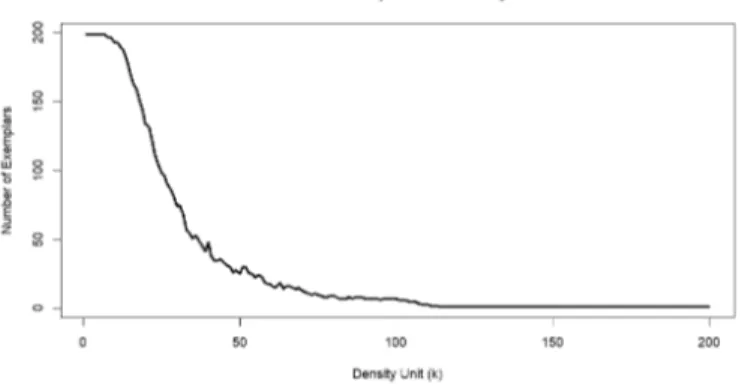
The number of selected exemplars decreases when the parameter value k increases. Fig.2 shows that the number of selected exemplars decreases from 200 to 1 when the density parameter k increases. This property of our method enables us to adapt a strategy to select the number of samples that we extract from the dataset. If we want a specific number of samples selected from the initial dataset, then we can adjust the parameter k to obtain the expected number of exemplars.

Fig. 2. Number of selected exemplars decreases from 200 to 1 when the density parameter k increases from 1 to 200

D. Assessment of the Method

The exploratory analysis of a dataset is complex for many reasons. The dataset is often divided into classes but the distribution of these classes is unknown. Moreover, the number

of these classes is also unknown. To better understand data, the use of a complementary exploratory trial on a smaller dataset is often necessary. The selection of a reduced number of samples should then represent all the classes of the dataset. For this reason, we will evaluate our sampling method under controlled conditions when the distribution of the classes is known. But of course, the method remains designed for applications in ex-ploratory analysis when the classes are unknown. This method is particularly useful when classes have large overlapping and when the classes have very different numbers of data. In such cases, the classical methods of clustering very often fail.

Let us consider a dataset with known distribution of classes for assessing our sampling method. We verify that the distribu-tion of the selected exemplars between classes remains com-parable with the distribution of data within the initial dataset. Table I gives the results we obtain with some simulations.

In the first five rows of the table, we use the dataset displayed in Fig.1. This dataset is simulated using four classes with a large overlapping. The 200 data are randomly distributed between these classes. (42, 51, 65, 42) is the distribution between the four classes. The number of selected exemplars decreases when the parameter k increases. We obtain 25, 18, 13, 9 and 7 exemplars using respectively 50, 60, 70, 80 and 100 as values of k. In these five simulations, the four classes are effectively represented by the exemplars. However, when k increases, the number of selected exemplars becomes too small for representing each class.

In the last five rows of Table I, we simulate five datasets with respectively 4, 5, 6, 7 and 8 classes. The number of data in each class is randomly selected and it could be very different from one class to another one. The datasets have 200 data and the parameter k is equal to 80 when selecting exemplars. When the number of classes increases, the number of exemplars becomes too small for representing each class (see the two last rows of the table). However, these classes are represented if the number of selected exemplars increases (i.e. if we decrease the value of the parameter k).

Let us study the sampling with real datasets. We consider some datasets of UCI repository (see in [5]). Table II displays the selection of exemplars using our blind method (i.e. when the classes are unknown) on the classical dataset called ”Iris”, ”Wine”, ”Glass”, ”Haberman” and ”Ecoli”.

These datasets have respectively 3, 3, 5, 2 and 8 classes. Our sampling method gives generally an exemplar in each class. Obviously the method fails if the number of classes is high compared to the number of selected exemplars. Moreover, the method often fails if the number of elements within one class is very low. For instance, in the last line of Table II, two classes have only 2 elements and these classes are not represented by any exemplar. But these classes can be represented by an exemplars if we increase the number of exemplars we select. For each of these datasets, we have measured the time to execute the algorithm with all possible values of k. It gives us the curves on Fig. 3. In this figure, for all k values, we show the time (in seconds) required to compute the exemplars. For more readability, we only show time values for k < 100 since

TABLE I

DISTRIBUTION BETWEEN CLASSES WITHIN A DATASET(n = 200)AND WITHIN THE SELECTED EXEMPLARS

Number of Distribution in dataset Number of Exemplars distribution classes (n = 200) selected between classes

exemplars 4 (42, 51, 65, 42) 25 (4, 8, 8, 5) 4 (42, 51, 65, 42) 18 (5, 6, 4, 3) 4 (42, 51, 65, 42) 13 (3, 3, 5, 2) 4 (42, 51, 65, 42) 9 (2, 3, 3, 1) 4 (42, 51, 65, 42) 7 (2, 2, 2, 1) 4 (7, 103, 62, 28) 10 (1, 3, 4, 2) 5 (40, 47, 55, 9, 49) 10 (2, 3, 2, 2, 1) 6 (6, 12, 76, 80, 24, 2) 9 (2, 1, 2, 1, 2, 1) 7 (23, 16, 51, 46, 1, 36, 27) 8 (1, 1, 1, 2, 0, 1, 2) 8 (37, 9, 3, 19, 48, 12, 45, 27) 9 (3, 0, 0, 1, 1, 1, 3, 1) TABLE II

DISTRIBUTIONS BETWEEN CLASSES WITH A REAL DATASET AND WITH SELECTED EXEMPLARS(n =NUMBER OF DATA, p =NUMBER OF VARIABLES) Name of n p Distribution Number of Distribution

dataset in dataset exemplars of exemplars Iris 150 4 (50, 50, 50) 8 (3, 3, 2) Wine 178 13 (59, 71, 48) 9 (2, 4, 3) Glass 214 9 (70, 76, 17, 13, 9, 29) 19 (1, 6, 1, 5, 1, 5) Haberman 306 3 (225, 81) 10 (7, 3)

Ecoli 336 7 (143, 77, 2, 2, 35, 20, 5, 52) 23 (3,9,0,0,3,3,2,3)

time execution is less than one second for each database.

Fig. 3. Execution time of the algorithm with different values of k

IV. APPLICATION TOVANETDATA

In this section, the scenario in which VANET data are collected and their description are provided. Then, the obtained results are presented.

A. Scenario and Data Description

In the Scoop@f [12] (Cooperative System at France) project, Intelligent Transport System (ITS) is experimented in the real life. To do so, connected vehicles drive on roadway and communicate with the infrastructure or other vehicles via a specific WiFi called ITS-G5. Messages used in Scoop@f are CAM [13] (Cooperative Awareness Message) and DENM [14] (Decentralized Environmental Notification Message). CAM is an application beacon with information about ITS station position, speed if it is a mobile station, etc. DENM is used to

warn about events. In this experimentation, the vehicle drives on a roadway and sends DENMs automatically. The event of this experimentation is a slippery road. When vehicle sends DENM, it logs the 30 previous seconds and 30 next seconds. We used these logs with our methodology.

The logs contain 3,201 data of 17 variables (7 for the acceleration control, the steering wheel angle, the strength braking and 8 for the exterior lights). The acceleration control is defined by the brake, gas and emergency brake pedals, collision warning, ACC (Adaptive Cruise Control), cruise control and speed limiter utilization. And the exterior lights are defined by the low and high beam, left and right turn signal (warning is the combination of both), daytime, reverse, fog and parking light.

B. Results

This subsection presents the results obtained with the ex-emplar selection method proposed previously. The objective is to describe characteristics from the experimentation and trying to model vehicle behavior on this type of road. By using the 3,201 data, we obtain results in Fig.4 where we can see that there is no big difference among data. This can be explained by the fact that roadway or highway has less variation than urban road. We then used our methodology with different values of k∈ {40, 80, 100, 140, 180, 200, 500}, which result in Table III. With k = 40, 142 samples are extracted, 102 with k = 80, 92 with k = 100, 58 with k = 140, 48 with k = 180, 46 with k = 200, and 18 with k = 500. The decrease in number of samples in comparison with the number of entries is explained by the fact that there is a lot of data that have equal values. With our methodology, a pre-processing is achieved by dividing by{22, 31, 34, 55, 66, 69, 178} the number of data to

be processed. This method can be very interesting for a pre-processing of big data in VANET.

Fig. 4. Profiles of 3,201 data with 17 variables from roadway experimentation.

k Number of exemplars Division 40 142 22 80 102 31 100 92 34 140 58 55 180 48 66 200 46 69 500 18 178 TABLE III

SELECTION OF EXEMPLARS WITH DIFFERENT VALUES OF THE

PARAMETERkFROM ROADWAY EXPERIMENTATION.

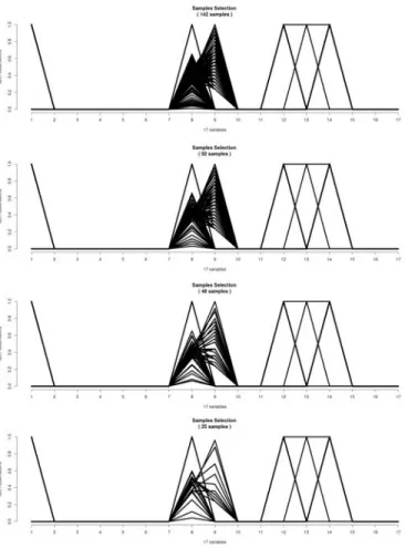
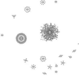
In order to illustrate the impact of variation of k to the number of representative samples, Fig.5 presents the obtained profiles while varying k (for more readability, only the samples are printed). It can be seen that it is very difficult to distinguish exemplars among data. To provide a clearer view, Fig.6 and Fig.7 present two extreme cases where one obtained with the smallest values (k=40) and another with the greatest value (k=500). In fact, these figures present the exemplars (central nodes) obtained with the algorithm and their connected neigh-bors (small nodes), and each number correspond to the number of the observation. It can be seen that the number of exemplars can be limited depending on the need of use case. When the value of k increases, the number of selected exemplars decreases. It has to be noticed here that the most important is to find the compromised tuning between the desired number of exemplars and the desired processing time and costs.

V. CONCLUSION AND FUTURE WORK

In this paper, we have presented a new methodology to select exemplars from a dataset containing multidimensional quantitative data. Our method is based on an estimation of the local density in a neighborhood of each data. With this methodology, it is also possible to select exemplars from classes, and then reduce the number of data in these classes. This methodology was first tested with random data and then with known real data. And, finally, it is applied to VANET data from the Scoop@f [12] project to perform exemplars of the situation described by the experimentation.

In the near future, we will use the methodology with other experimentations and will develop tools to create classes representing each experimentation. Furthermore, this work is

Fig. 5. Profiles of 3,201 data with 17 variables from roadway experimentation with varying values of k.

Fig. 6. Data Network with k=40

a contribution for designing tools to analyze data of roadway experimentations in the project Scoop@f.

Fig. 7. Data Network with k=500

ACKNOWLEDGEMENT

This work was made possible by EC Grant No. INEA/CEF/TRAN/A2014/1042281 from the INEA Agency for the SCOOP project. The statements made herein are solely the responsibility of the authors.

REFERENCES

[1] Frixione, M., Lieto, A.: Prototypes Vs Exemplars in Concept Represen-tation. Int. Conf. on Knowledge Engineering and Ontology Development KEOD (2012)

[2] Frey, B.J., Dueck, D.: Clustering by Passing Messages Between Data Points. Science Vol. 315, 972–976 (2007)

[3] Cochran, W.G.: Sampling Technique. Ed. Wiley Eastern Limited (1985) [4] Houle, M.E., Kriegel, H.P., Kroger, P., Shubert, E., Zimek, A.: Can Shared-Neighbor Distances Defeat the Curse of Dimensionality? Proc. 22th Int. Conf. on Scientific and Statistical Database Management, Ed. Springer (2010)

[5] Bache, K., Lichman, M.: UCI Machine learning repository.

http://archive.ics.uci.edu/ml, University of California, Irvine, School of

Information and Computer Sciences (2013)

[6] Nadem T, Shankar P, L. Iftode;: A Comparative Study of Data Dissemina-tion Models for VANETs 3rd Annual InternaDissemina-tional Conference on Mobile and Ubiquitous Systems (MOBIQUITOUS), July 2006.

[7] Mekki T., Jabri I., Rachedi A. Benjemaa M. Vehicular cloud networks: Challenges, architectures, and future directions. Elsevier Vehicular Com-munications, Volume: 09, pp.268-280, 2017.

[8] Rachedi A., Badis H. BadZak: An hybrid architecture based on virtual backbone and software defined network for Internet of vehicle. IEEE International Conference on Communications, May 2018, Kansas City, United States, 2018.

[9] Castellano A., Cuomo F.: Analysis of urban traffic data sets for VANETs simulations CoRR abs/1304.4350 (2013)

[10] Ramassamy C., Fouchal H., Hunel P. Classification of usual protocols over wireless sensor networks Communications (ICC), 2012 IEEE Inter-national Conference on, 622-626

[11] Bernard T., Fouchal H. Slot scheduling for wireless sensor networks Journal of Computational Methods in Sciences and Engineering 12 (s1), 1-12

[12] Scoop@f: http://www.scoop.developpement-durable.gouv.fr/

[13] CAM: ETSI EN 302 637-2; Intelligent Transport Systems (ITS); Ve-hicular Communications; Basic Set of Applications; Part 2: Specification of Cooperative Awareness Basic Service. European Standard. ETSI, Nov. 2014.

[14] DENM: ETSI EN 302 637-3; Intelligent Transport Systems (ITS); Ve-hicular Communications; Basic Set of Application; Part 3: Specifications of Decentralized Environmental Notification Basic Service. European Standard. ETSI, Nov. 2014.

[15] Heinrich, J., Weiskopf, D.: State of the Art of Parallel Coordinates. STAR ? State of The Art Report, Visualization Research Center, Univer-sity of Stuttgart, Eurographics (2013)

[16] Garcia, S. and Derrac, J. and Cano, J. & Herrera, F. (2012).Prototype selection for nearest neighbor classification: Taxonomy and empirical study. IEEE transactions on pattern analysis and machine intelligence, 34(3), 417-435.

[17] Pkalska, E., Duin, R. P., & Paclk, P. (2006). Prototype selection for dissimilarity-based classifiers. Pattern Recognition, 39(2), 189-208. [18] P. Grother, G.T. Candela, and J.L. Blue, Fast Implementations of

Nearest-Neighbor Classifiers, Pattern Recognition, vol. 30, no. 3, pp.459-465, 1997

[19] Kim, B. S., & Park, S. B. (1986). A fast k nearest neighbor finding algorithm based on the ordered partition. IEEE Transactions on Pattern Analysis and Machine Intelligence, (6), 761-766.