Numerical simulation of resin transfer molding using linear boundary element method

(1)

HAL Id: hal-01716290

https://hal.archives-ouvertes.fr/hal-01716290

Submitted on 26 Mar 2019

HAL is a multi-disciplinary open access

archive for the deposit and dissemination of

sci-entific research documents, whether they are

pub-lished or not. The documents may come from

teaching and research institutions in France or

abroad, or from public or private research centers.

L’archive ouverte pluridisciplinaire HAL, est

destinée au dépôt et à la diffusion de documents

scientifiques de niveau recherche, publiés ou non,

émanant des établissements d’enseignement et de

recherche français ou étrangers, des laboratoires

publics ou privés.

Numerical simulation of resin transfer molding using

linear boundary element method

Fabrice Schmidt, P Lafleur, Florentin Berthet, Pierre Devos

To cite this version:

Fabrice Schmidt, P Lafleur, Florentin Berthet, Pierre Devos. Numerical simulation of resin transfer

molding using linear boundary element method. Polymer Composites, Wiley, 1999, 20 (6), pp.725-732.

�10.1002/pc.10396�. �hal-01716290�

(2)

Numerical Simulation of

Resin Transfer Molding Using

Linear Boundary Element Method

F.

M. SCHMIDT

EnStimac

Route

de

Teillet,

81

01 3

Albi CT

Cedex 09,

France

P. LAFLEUR

CRASP,

E€ok Polytechnique

Montreal,

QC, H3C

3A7,

CQnada

F. BERTHET

EnStimac

Route de

Teillet,

81 0 1 3 Albi

CT Cedex

09,

France

P.

DEVOS EnStimac

Route de

Teillet,

81 01 3 Albi

CT

Cedex

09,

France

Using mass conservation and Darcy's law to describe flow through isotropic porous media leads to a Laplace equation, which may be solved numerically at

each time step using the boundary element method. For anisotropic porous media

in which the permeability matrix is symmetric, the problem can be solved in the same way by rotating and stretching the coordinates. The numerical model has been compared with analytical solutions and experimental data in the case of radial

front flows and with finite element for a frontal injection.

1 INTRODUmION

he resin transfer molding

(m

process has be-

T

come popular in a variety of industries: sporting goods, defense, military, automotive, and aerospace

(1, 2). It is widely used in the manufacturing of large components of fiber reinforced materials. BasicaUy it is a two-step process. In the first step, a fiber preform composed of several layers of fiber mats or woven rov- ing is produced. In the second step, the resin is injected into a mold filled with the preform. The resin enters the mold through one or several injection gates and impregnate progressively the preform with or without vacuum assistance.

The main advantage of this process in comparison with others is its adaptability. This process makes it

possible to produce simultaneously a component and a material that perfectly fit the property requirements

locally and globally (3). This is done by combining a

variety of fiber types, levels, and architectures with a variety of cores and resins.

Because of its economic interest, this process has replaced traditional lay-up of prepregs for some appli- cations (in particular to avoid time and labor expensive surface preparation prior to painting). Even though components are industrially produced, the fill-

ing

step is still not very well understood and therefore predicted. The mold materials are seldom transparent so that the flow cannot be visualized, and it is very difficult to determine how the resin will flow and impregnate the preform. Roper design of the vent and injection port location is crucial to prevent large air

pockets from being trapped during flow (if no vacuum assistance is used). The more complicated the mold, the more difficult (and also expensive) it is to adjust

(3)

F.

M. Schmidt, P.

LaJZeur, F.

Berthet, and P. Dews

the gates’ locations. This difficult task becomes an ex-

pensive one if it is done by a trial and error method. Problems can be anticipated by a proper process simulation. The numerical analysis of resin flow in the mold is a very important (technical and economical) task in designing the RTM mold and to understand the impregnation of the preform.

Several numerical methods have been developed to simulate the filling step of FClM. Cai (4) has developed

a simplified

filling

simulation for both Newtonian and power law fluid with a 1D flow closed form solutions.

Using geometry simplifications and an assemblage of mold sections, the total filling time, the inlet pressure or flow rate was calculated. The calculation showed a

good agreement with Coulter and Giiceris TGMOLD

(5). Methods based on 2D finite difference have been used by Li and Gauvin (6) and by Coulter et al. (7, 8). The authors themselves notice the difficulty of finding realistic boundary conditions and point out the limita- tion of these methods for FClM. _{Finite element meth-}

ods have been used by many authors as Trochu et al.

(9) or Hoareau (1 0). The control volume method has been used by Lee et al. (1 1). These methods have the disadvantage of needing the meshing of either the whole preform or of the wetted region of the preform. Many authors have chosen a 2D formulation because the thickness of the component for impregnation is small in comparison with other dimensions. Neverthe- less, Young et al. (12) have developed a 3D formulation of the finite element method with control volume method for thick components. With this coupled technique, remeshing at each time step is avoided and only the domain of calculation is recalculated at each time step.

In this study, following Um and Lee (13) and Hada- vinia et al. (14), the resin flow will be solved numerically by the boundary element method

(BEM).

Tmdi- tional boundary element methods are particulaxy suitable for solving linear problems (Newtonian fluids). However, the methods have also been extented to solve nonlinear problems by iterative or incremental procedures. The variation of the boundary element method for a wide range of nonlinear problems in- cluding non-Newtonian fluids flows have been de- scribed in detail elsewhere (15, 16). and here we will

only describe the technique when the resin is considered Newtonian. The results of numerical calculation will be compared to numerical solutions available for centrally injected anisotropic porous media. The numerical simulations will also be compared to finite elements results and experiments.

2 GOVERNING EQUATIONS

The impregnation of a fibrous preform is usually modeled as a flow through anisotropic homogeneous porous media and is governed by Darcy’s law

K:;

21

the where

3

is the velocity vector, [K] =

permeability tensor, p the resin pressure and p the viscosity (constant for a Newtonian resin). Combining Eq 1 with the continuity equation gives:

w3

-+

7. (-

v

p) = 0

Equation 2 can be reduced to Laplace’s equation by rotating and stretching the coordinates. The trans-

formed coordinat s 2 m a y be deduced from the sys- tem coordinates

4

using the following relationship:

r

a 1 ~ 3 ,

-I

where (a1.

pl,

az,

pz)

and (Al,

A2)

are the components of the eigenvectors and the eigenvalues of the permeability matrix, respectively, and K, = the equivalent permeability. Using the coordinates

?

Eqs

1 and 2 can be rewritten as:

(4)

A p = O (5)

2.1c9lcolrtlonafpnAnalyticp1Qolutioll

Let u s consider the radial impregnation of an aniso-

tropic fibrous medium by an incompressible New- tonian fluid. Equations 4 and 5 are available. Using

cylindrical coordinates, in 2D relative to the principal directions, the pressure can be calculated from Eq 5:

where po and pfrepresent the inlet and front pressure respectively whereas R, and %are the inlet and front

radii. Fluid velocity, in the new system of coordinates,

can be obtained from (4):

(7) The flow front velocity is given by the relationship between the phase (fluid) average u to the intrinsic phase average V (front velocity) ( 1 7).

726

where E is the system porosity. If we assume that the porous medium is anisotropic and homogeneous, the

(4)

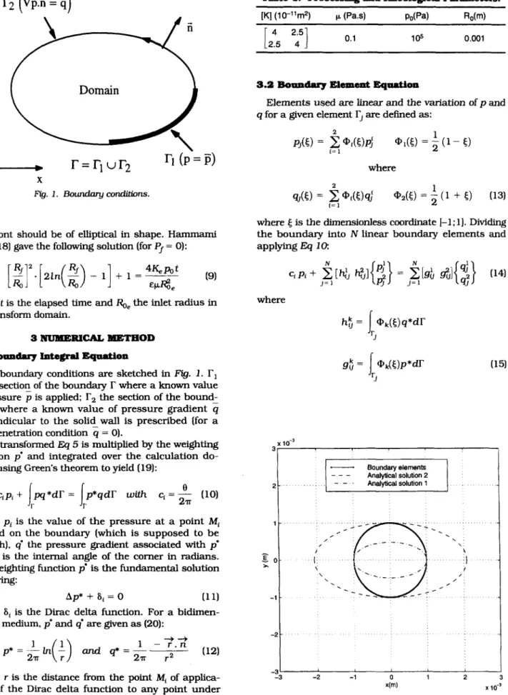
Table 1. Processing and Rheological Parameters.

yt

I-,

r=rlur2

r1

(P

=

Y A

m.

1 . Boundary conditions.

flow front should be of elliptical in shape. Hammami

et

aL

(18) gave the following solution (for Pr = 0):

[ 3 [ 2 1 n ( 3 - 11

+

1 =- 4K,

Po

(9)

wee

where

t is

the elapsed time and

be

the inlet radius in

the transform domain.

3NUMERXCALlllLETHOD 3.1 Boundary Integral Equation

The boundary conditions are sketched in FSg. 1 . is the section of the boundary

r

where a known value of pressure is applied:

rz

the section of the bound-

ary

r

where a known value of pressure gradient

4

perpendicular to the solid wall is prescribed (for a non-penetration condition

4

= 01.

The transformed

I

Q

5 is multiplied by the weighting function p' and integrated over the calculation do-

main using Green's theorem to yield (19):

where pi is the value of the pressure at a point Mi located on the boundary (which is supposed to be smooth),

6

the pressure gradient associated with p' and 8 is the internal angle of the comer in radians.

The weghting function p' is the fundamental solution satisfying:

A p *

+

6 , = 0 (1 11

where 6 i is the Dirac delta function. For a bidimen- sional medium, p' and q' are given as (20):

where r is the distance from the point M i of application of the Dirac delta function to any point under consideration.

[K] (10-'lrn2) p (Pas) P O P 4 RO(@ 105 0.001

3.2 Boundary Element E q d m q for a given element

rj

are defmed as:

Elements used are

linear

and the variation of p and

where

6

is the dimensionless coordinate [-l;l]. Dividing the boundary into

N

linear boundary elements and applying

m

10:

-

Boundary elements Analytical solution 2 Analytical solution 1 1 -

-

L 0 - k -1 -

I

-3 -3 -2 -1 0 1 2 3

FYg. 2. Circular inlet between two ellipses.

(5)

F.

M.

Schmidt, P. Jhjkur,

F.

Berthet, and P. Deuos

Since pressure is unique at any point: resin front is updated using a forward Euler integra-

Equation 14 can be rewritten in matrix form as:

(16) where:

N, = %-l + wj + b j c ,

Fluxes are unique at any point of smooth surfaces and unknown after or before a comer (transition from known pressure to known flux or vice versa). As long

as there is only one unlcnown per node, a NZN system

can be obtained. Such a system can be reordered as:

A x =

F (17)

where X is the vector of N unknowns, A is a NZN ma- trix obtained by reordering G and H. F is the known

vector computed from the boundary conditions and the Nand G matrices.

3.3 Reain Front

updating

At each time step AC the flow of resin inside the mold is regarded as quasi-steady. Unknown pressure p and pressure gradient q on the boundary are calcu- lated by using Eq 17. Then, the new location of the

Rg. 3. Comparison between BEM and analytical flow fronts (t =

200 d.

tion scheme:

(181

+

_{x ( t +}_At)₌

_?(t)

₊

_{A t (}

+ + +

u . n ) n

On the resin front, only the n o d component of the resin velocity is needed since there is no tangential component of the velocity. Combining Eqs 4 and 18 we obtain:

x ( t + At) = ?(t) - A t

+

In addition, the nodes close to the mold are relocated using an orthogonal condition.

4 MODEL ASSESSMENT

The boundary elements method developed for the FCIM process was compared to analytical solutions, fi-

nite element simulations and experimental data. The

first case considered was the central injection of a n anisotropic and orthotropic fibrous medium. The porous media was rotated with an angle of 45" for a pur- pose of generality. The values of the different param-

eters used are given in Table 1.

The matrix

[Kl

is the permeability matrix in the

2

coordinates system. It is the expression of the princi-

pal permeability matrix O

]

rela-

1, 5.10-"

tive to coordinates such as

(2

3

= 45". The flow front should be of elliptical shape. The half-lengths

%

and

0.08 -. . <. . .. . . * . . . .. . . .. . . ... ... ... ... .

..

. . .. . .

..

. . . ... ... . . .

..

. . .

..

. . .

(6)

m.

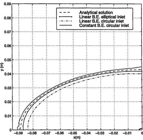
4 . Comparison b e t w e e n lin-

ear and _{contant BEM}_and_analyti- c d f i w j f o n t s . 0.09 0.08 0.07 0.06 ! I I I I Analytical solution Linear B.E. circular inlet Constant B.E. circular inlet

-

...

!

...

Linear

B.E.

elliptical inlet

...

.-.-.-

-

...

-..

.

...

.

...

.:.

...

:.

...

.<

...

..i

...

i..

...

:.

...

.i..

...

;

{

h

Table 2. Processing and Rheological Parameters. E Y >. / I (

i

0 I ' I I I I I I I -0.09 -0.08 -0.07 -0.06 -0.05 -0.04 -0.03 -0.02 -0.01 0 x(m) 105 0.001

%p of the principal axis of the ellipse can be com-

puted with Eq 9. The half-lengths of ellipses are re- lated to principal permeabilities by:

In Eq 9, the pressure po is applied in the

2

system coordinates which implies an elliptical inlet. In fact, there is two possible elliptical inlets. Ifwe proceed to a

BEM simulation with a circular inlet located between these two ellipses (see Fig. 2). the BEM flow front should be located between the analytical flow fronts corresponding to these ellipses.

Figure 3 shows the comparison between the flow front which has been computed

using

the boundary element method with h e a r elements and the an-- cal solutions at t = 200 s for ellipses of half axes (0,00208: 0.001) and (0,001: 0,00048). The time step used for the numerical simulation is A t = 0 . 1 s and the CPU time for the complete simulation is one minute on IBM Risk 6000. The simulation is in good agreement with the analytical solution and the calculated flow front is located between the analytical solu-

tions corresponding to the half-axes. m u r e 3 also shows the sensitivity of the method to the selected inlet geometry. A small variation of the inlet geometry has important role on the shape of the flow front posi- tion.

In Fig. 4, different boundary element simulations are shown for an orthotropic case for one quarter of the domain. The values of the processing and rheological parameters are given in Table 2.

The boundary element simulation with constant elements leads to some problems close to the mold wall

(Fig. 4). Moreover, it overestimates the flow front posi- tion. Linear elements improve the contact description. Two different inlet geometry were compared: a circular inlet and an elliptical one. The difference between the

boundary element method and the analytical solutions can be explained by the sensitivity of the inlet geometry.

4.2 Cornparimon W i t h Finite Element Simulation

A second system consisting of a frontal injection of resin into a fibrous preform located between two par- allel solid walls was used to compare k i t e element and boundary element methods. The resin was as- sumed to be an incompressible Newtonian fluid flow-

ing

through an anisotropic one layer medium.

The finite element simulation has been carried out

using

a numerical model first developed by Hoareau

et aL (21) and derived from FORGE2@, software. The numerical model is based upon an updated lagrangian

finite element method (FEM). The domain is meshed

(7)

F. M. Schmidt, P. L.u@ur,

F.

Berthet, and P. Devos

q=o

Fig.5. Finiteelementmeshatt=200s.

agreement for linear elements. The discrepancy between the BEM and FEM flow fronts increases in the lower part.

4.3 Cornpariaon With Experimental Data

Experimental data available for the case of central injection into a transparent mold was used to compare BEM and experimental measurement. The dimensions of the mold are 0.5 m per 1 m (Rg. 7) and

a silicone oil resin was used to impregnate an isotropic fibrous medium made of six layers of OCF 86 10 fiber mat. All details of the procedure can be found in

reference (22). The values of the processing and rheological parameters are given in Table 3. The CPU time for the complete simulation is 2 min. The agreement between the BEM and the experimental data is fair

except near the walls. The numerical flow fi-onts shown

in Fig. 8.a are symmetric while the experimental ones are non-symmetric ( R g . 8.b). This is due to the dif- ficulties of placing the preform of reinforcing fibers perfectly in contact with the mold walls. The permeability will increase near the wall generating preferen- tial flows.

5 CONCLUSION

5. The values of the processing and rheological parameters are the same as the one given in Table 1 .

The CPU time for the FEM simulation is about half- an-hour. As shown in Fig. 6, the agreement is fair for both constant and linear boundary elements except close to the lower wall. As expected, we have a better

The flow of a Newtonian resin through anisotropic and homogeneous media has been simulated using a

boundary element method. The algorithm which is

used to capture the transient h n t flow is rather sim- ple and can accurately predict the front shape at a

Rg. 6. Comparison between BEM

and FEMjlowfronts at t = 200 s.

(8)

Numerical Simulation of KlM

clamping

/

Fg. 7. Cross section of the ex- perimental mold-h thickness of

the mold

base

Plexiglas

sheet

Table 3. Processing and Rheological Parameters. [K] (104m2) fi (Pas) P C W ) %(m)

15 0.01

Fg. 8. Comparison between BEM

simulations la) and experiments

m.

\

fiber mats

low cost. The numerical model has been validated by comparison with analytical solutions for a central in- jection and with finite element for a frontal injection. The anisotropic and orthotropic fibrous medium have been investigated. I I I I I I I

.

I I . .~ . . . . . I " I ' . . . . . . I ' . / . . . I . . . I . / J . . I . . -0.15 . . . . . . ,./ . . . . I . / / I . . . . . . I . / '

,

-0.25

I

I I I I / I I I I 1 I

1

0 0.1 0.2 0.3 0.4 0.5 0.6 0.7 0.8 0.9 1 x(m)

..-..

I

:'14.SS'..

37

6 :

53.5s:

8 2 - 5 6

(9)

F.

M.

Schmidt, P.

LaJlau;

F.

Berthet, and P. Devos

Preliminary comparison with experimental data available for the case of central injection into a trans-

parent mould have been processed. However, further comparisons between BEM simulations and experi- ments are needed to improve the model.

In

particular, the relocation scheme used for the nodes close to the mold has to be improved in order to take into account the contact between the resin and the mold.

Further developments will allow the simulation of the flow of resin through a typical FClW reinforcement (i.e. inhomogeneous porous media). The boundary ele- ment method will be applied to each subregion (as- sumed to be piecewise homogenous) as if they were independent of each other.

REFERENCES

1. C. F. Johnson, N. G. Chavka, R A. Jeryan, C. J. Monis, a n d D. A. Balbington, Design a n d fabrication of a HSRTM crossmember module, proceedings of the third

annual ASM/ESD advanced Composites Conference, 2. A. Arnold and W. Becker, RTM: simultaneous design and tooling reduces cost and lead time, proceedings of

the 23rd International SAMPE Technical Conferences

(1991).

3. D. A. Steenkamer, The innuence of preform design and manufacturing issues on the processing and perfor- mance of resin transfer molded composites (Volume I

and II). Thesis of Uniuersitg of Delaware (1994).

4. Z. Cai, Simplified mold filling simulation in resin trans-

fer molding, Journal of Composite Materials, Vol. 26, No

5. J. P. Coulter and S. I. Guceri, resin transfer molding: process review, modeling and research opportunities- Proceedings of M a n u f w International 88, Atlanta GA, N04. p. 79, 86 (1988).

6. S. Li and R. Gauvin, Numerical Analysis of the Resin Flow in Resin Transfer Molding. Journal of Reinforced 7. J. P. Coulter and S. I. Guceri, resin impregnation dur- ing the manufacturing of composite materials subject to prescribed injection rate- Journal of reinfmced plastics

and composites, May, Vol. 7, p. 200-219 (1988). 8. J. P. Coulter and S. I. Guceri, resin impregnation dur-

ing composites manufacturing: theory and experimenta- tion, Composites Science and Technology, Vol. 35, p. pp. 197-217 (1987).

17, p. 2606-2630 (1992).

Plnstics and C o m p o ~ i t e ~ , Vol. 10, 314-327 [May 1991).

317-330 (1989).

9. F. Trochu, R. Gauvin, Gao Dong Ming, and J.-F. Boud- r a u l t , RTMFLOT, An Integrated Software Environment for the Computer Simulation of the Resin Transfer Mold- ing Process. Journal of Reinforced Plastics and Com-

10. C. Hoareau, F. Trochu, R Gauvin, and M. Vincent, Proc.

11. L. James Lee. W. B. Young, and R J. Lin, Mold filhng and cure modelling of and SlUM processes. Corn-

posites structures, Vol. 27, 109-120 (1994).

12. W. B. Young, K. H. L. M. Fong, L. J. Lee, and M. J. Liou, Flow simulation in molds with preplaced fiber mats,

pdymer Composites. 12. p. 391 (1991).

13. M.-K. Um and W. I. Lee, A study on the Mold Filling Process In the Resin Transfer Molding. Polymer Engi-

neering and Science, Vol. 31, No. 11, 765-771 (Mid- June, 1991).

14. H. Hadavinia. S. G. Advani, and R. T. Fenner, The evo- lution of radial fingering in a hele-Shaw cell using C1

continuous Overhauser boundary element method.

Engineering Analysis Boundary Elements, Vol. 16, 183- 195 (1995).

15. M. B. Bush, The application of Boundary Element Method to Some Fluid Mechanics Problems, PhD Thesis, University of Sydney ( 1984).

16. R. Zheng, Boundary Element Method for some problems

in Fluid Mechanics and Rheology, PhD Thesis, University 17. C. L. Tucker, 111, and R. B. Dessenberger, "Chapter 8:

Governing equations for flow and heat transfer in sta-

tionary fiber beds," Flow and rheology in polymer corn- posites manufacturing edited by s. G. Advani, Elsevier Science B. V. (1994).

18. A. Hammami, F. Trochu, R. Gauvin & S. Wirth. Direc- tional Permeability Measurement of Deformed Rein- forcement. J. of Reinforced Plastics and Composites. Vol.

15 (June 1996).

19. C. A. Brebbia and J. Dominguez, Boundary Element: An

introduction course. McGraw-Hill Book Company, Sec- ond edition (1992).

20. N. Ozisik, Heat Conduction, J o h n Wiley & Sons (1980). 21. C. Hoareau, Injection sur renfork etude du remplissage

de moule et d&rmination t h b r i q u e de la permbbilite des tissus, t W s e d e doctorat de l'ecole d e s mines de Paris, in French (1994).

22. Zhang, Zheng, * Simulation par elements h i s du rem- plissage des moules par le p r o c i d t de moulage par transfert de resine.. Memoire d e Maitrise, in French, h l e Poytechnique de Montrt5al( 1992).

posites, Vol. 13. 262-270 (March 1994).

Of ICCM-9. M a d r i d Vol. 3. pp. 481-488 (July 1993).

of Sydney (1991).

732 POLYMER COMPOSITES, DECEMBER 1999, Vol. 20, No. 6

Powered by TCPDF (www.tcpdf.org) Powered by TCPDF (www.tcpdf.org) Powered by TCPDF (www.tcpdf.org) Powered by TCPDF (www.tcpdf.org) Powered by TCPDF (www.tcpdf.org) Powered by TCPDF (www.tcpdf.org) Powered by TCPDF (www.tcpdf.org) Powered by TCPDF (www.tcpdf.org)