Validation of a New Finite Element for Incremental Forming Simulation
Using a Dynamic Explicit Approach
C. Henrard1, C. Bouffioux2, L. Duchêne3, J.R. Duflou4 and A.M. Habraken1
1 Université de Liège, Department ArGEnCo - MS2F, Chemin des Chevreuils 1, 4000 Liège, Belgium 2Vrije Universiteit Brussel, Department MeMC - TW, Pleinlaan 2, 1050 Brussels, Belgium
3Royal Military Academy, Department COBO, Avenue de la Renaissance 30, 1000 Brussels, Belgium 4Katholieke Universiteit Leuven, Department PMA, Celestijnenlaan 300A, 3001 Heverlee, Belgium
Abstract: A new method for modeling the contact between the tool and the metal sheet for the incremental
forming process was developed based on a dynamic explicit time integration scheme. The main advantage of this method is that it uses the actual contact location instead of fixed positions, e.g. integration or nodal points. The purpose of this article is to compare the efficiency of the new method, as far as accuracy and computation time are concerned, with finite element simulations using a classic static implicit approach. In addition, a sensitivity analysis of the mesh density will show that bigger elements can be used with the new method compared to those used in classic simulations.
Keywords: Finite Element Method, Dynamic Explicit, Incremental Forming
INTRODUCTION
Single point incremental forming (SPIF) is a sheet metal forming process that is very appropriate for rapid prototyping because it does not require any dedicated dies or punches to form a complex shape. Instead, it uses a standard smooth-end tool mounted on a numerically controlled multi-axis milling machine. The tool follows a complex tool-path and progressively deforms a clamped sheet into its desired shape [1,2].
Simulating this process is a complex task. First, the tool diameter is small compared to the size of the metal sheet. Moreover, during its displacement, the tool deforms almost every part of the sheet, which implies that small elements are required everywhere on the sheet. For implicit simulations, the computation time is thus prohibitive. In this article, the simulations were performed using the finite element code Lagamine developed at the University of Liège [3]. In order to decrease the simulation time, a new method using a dynamic explicit time integration scheme has been developed.
This article begins by briefly summarizing the new developments introduced in the finite element code used. Then, it presents the reference simulation, the line test, used throughout this article. The next three sections present the results obtained for the prediction of the shape, the force on the tool and the computation times. Finally, some conclusions are drawn, followed by future perspectives.
NEW DEVELOPMENTS: MST
Classic finite elements use a penalty method to model contact between the tool and the sheet [4]. This approach has several drawbacks, the most important one being the fact that the penalty coefficient must be as large as possible in order to be accurate and reduce the remaining interpenetration. Since the coefficient is added to the stiffness matrix, that matrix becomes ill-conditioned, leading to a poor convergence of the implicit simulations. The new method, called MST (Moving Spherical Tool), uses a dynamic explicit time integration scheme. Without damping, and if a diagonal (or lumped) mass matrix is used, the solution of the equilibrium equation is straightforward:
where = inertia forces,
= internal forces, equivalent to the stress state, = external forces.
A typical explicit time step is presented in Fig. 1. The innovative part of this method concerns the way the contact forces are taken into account. First, they are ignored when solving the equilibrium equation. Then, the error in the contact with the tool is computed geometrically. This depends only on the position and velocity of the nodes close to the tool at the end of the time step. Finally, the nodal acceleration at the beginning of the time step can be corrected in order to meet the required contact conditions at the end of the time step. The correction on the acceleration, multiplied by the nodal mass, is equivalent to the contact forces.
Fig. 1: Dynamic explicit time step
Compared to a more classic approach, the main improvement here consists in being able to take into account a point of contact anywhere inside the elements without using penalty. Moreover, a special strategy is used to keep track of the nodes close to the tool from one step to the other. More information about this method can be found in a previous article by the author [5].
REFERENCE SIMULATION: LINE TEST
The validation of the new approach will now be performed on the so-called line test simulation. This simple SPIF test is presented in Fig. 2. Starting with the tool tangent to the top surface of the metal sheet, the tool-path is composed of three steps: a 5 mm indent into the sheet metal (A→B), a 100 mm line along the x-axis (B→C) and the unloading (C→D). These three steps are respectively performed in 0.2, 0.6 and 0.2 seconds.
The tool diameter is 10 mm. The thickness of the sheet is 1.2 mm. The material used is an Aluminum alloy AA3003-O with p =2700 [kg/m3], E=70000 [MPa], v=0.33 and σ0=33 [MPa]. Its yield locus is modeled using a
Hill law (F=1.22; G=1.19; H=0.81 and N=L=M=4.06) and the hardening is considered isotropic and follows a Swift-type law
where σF is the yield stress and εpl, the plastic strain. The parameters were chosen equal to K=183, ε0=0.00057
and n=0.229.
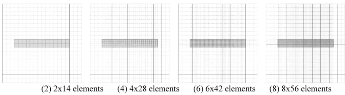
Four different meshes were tested, as presented in Fig. 3. The smallest element sizes (expressed in mm) are respectively: (2) 9.1x 9.1; (4) 4.55 x 4.55; (6) 3.03 x 3.03 and (8) 2.28 x 2.28. Two different element types were used: an eight-node brick element with one integration point called BWD3D [6,7], and a four-node shell element with six degrees of freedom for each node - three translations and three rotations - called COQJ4 [8]. In the case of brick elements, three layers of elements were used along the thickness.
The boundary conditions simply consist in clamping the sheet along its four edges. For brick elements, all the nodes along the thickness were fixed; as for shell elements, the nodes were fixed only in translation, not in rotation.
As far as the time integration scheme is concerned, both the classic static implicit and the new dynamic explicit schemes were tested.
Fig. 2: Schematic presentation of the line test
Fig. 3: Four meshes used for the line test with the number of elements in the center region
SHAPE RESULTS
Comparison of integration schemes and element types.
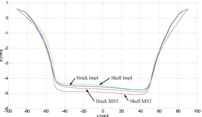
In this section, the shape of the metal sheet will be analyzed in a cross-section along the tool-path for the finest mesh (number 8 in Fig. 3) at two different instants during the simulation, i.e. after the indent and when the tool arrives at the end of the line. In the case of the brick elements, the average vertical position of the nodes along the thickness is presented. Those results are shown in Fig. 4 and 5. Four simulations are compared: implicit (with contact using penalty) and dynamic explicit (with MST algorithm), both with brick and shell elements.
After the indent, the results of all simulations are quite similar (deviation of maximum 0.2 mm), except around the boundary conditions. This is due to the fact that the rotational degrees of freedom of the shell elements were not fixed. It has been proved that if the six degrees of freedom are fixed, the shape is closer to the brick
simulation around the edges.
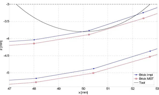
At the end of the line, however, the situation is quite different. There is a maximum deviation of 0.5 mm between the shell implicit and the shell MST. This variation may either be due to the difference in the contact treatment or to the time integration scheme. The MST algorithm has been designed to model the contact accurately. Its efficiency can be seen in Fig. 6, where the top and bottom surfaces of two simulations performed with brick elements are presented. The implicit simulation shows interpenetration, whereas the MST exhibits perfect contact.
Fig. 4: Shape shown in a cross-section after the indent
Fig. 6: Zoom on the contact region between the tool and the metal sheet
The deviation between the curves in Fig. 5 must therefore result from the time integration algorithm. Indeed, with the explicit algorithm, the simulation is conditionally stable, i.e. the time step has a maximum value, which is given by the equation
for shell and brick elements, respectively. Δtc is the critical time step and Lmin is the smallest element dimension
in the mesh. Without mass multiplication and for the finest mesh (number 8 in Fig. 3), this relation leads to time steps of the order of magnitude of 4.10-7 s for shell and 6.10-8 s for brick elements. The number of time steps required to reach the final time of 1.0 s is huge. For the simulation presented, a mass scaling factor of 20 was used. The time steps increase, i.e. 2.10-6 and 3.10-7 s approximately, but the inertia terms also become larger, leading to bigger errors. In this matter, the major difference between shell and brick elements stems from the fact that the smallest element dimension in the shell mesh is in the plane of the sheet, whereas it is one third of the thickness (since three brick elements are used in that direction) for brick elements. This fact reduces
considerably the number of time steps to be performed with shell elements.
Mesh size influence.
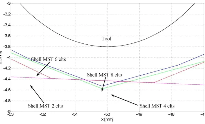
This section examines the influence of the mesh size on the results of the simulations. Fig. 7 shows a zoom on the tool after the indent for the four meshes seen in Fig. 3 with shell elements using the MST algorithm. (It should be noted that neither the thickness of the elements nor their curvature is shown in this figure, but is taken into account by the program.) It can be seen that small differences appear, depending on the mesh size. In particular, meshes 4 and 8 have a node under the tool, which results in a negative peak. However, that temporary error no longer appears when the tool is at the end of the line, as can be seen in Fig. 8. Except for mesh 2, which is too coarse, and to a lesser extent mesh 4, the deviation between the results is small. As a result, one may conclude that a relatively coarse mesh can be used with the MST algorithm.
Fig. 7: Zoom on the tool after the indent for four different shell meshes
Fig. 8: Tool at the end of the line for four different shell meshes
FORCE RESULTS
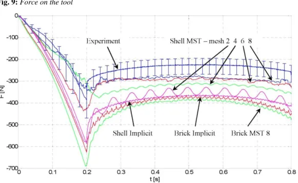
In this section, the prediction of the tool force is analyzed. In Fig. 9, the evolution of the vertical component of the tool force is presented for different simulations, along with the experimental measurement - and its variation - performed in Leuven (Belgium) by the team of Prof. J.R. Duflou. As can be observed in the graph, the best results are obtained with shell elements using the MST algorithm and the finest mesh, whereas the brick elements predict a much higher force. This result seems logical for two reasons: first, the shell element is inherently better adapted to modeling sheet metal forming processes; second, the MST algorithm has been
designed to adjust the contact forces in order to get perfectly accurate geometrical results. It can also be observed that the coarser the mesh, the greater the oscillations in the force.
To conclude this section, it may be mentioned that the only drawback to the MST algorithm in force prediction is that parasitical oscillations appear due to the explicit integration scheme. A smoothing of the curves1 is therefore necessary.
Fig. 9: Force on the tool
COMPUTATION TIMES
In this section, the computation times are shown in hours2 for different simulations (Table 1). The most important remark to be made here is that the MST algorithm is slower than the classic implicit algorithm. For shell elements, however, this difference is much smaller than for brick elements, where the computation times are so significant as to be unacceptable. Therefore, time efficiency is another advantage of shell elements.
Table 1: Computation times in hours
Implicit MST
Brick 41 5793
Shell 18 129
The reason why the MST algorithm is slower than the implicit one is that the number of time steps is far more substantial and the Lagamine code is not optimized for explicit computation.
1
The smoothing was performed using a moving average algorithm.
2 If
CONCLUSIONS AND PERSPECTIVES
This article presents the validation of a new dynamic explicit code. The main characteristic of this code, as compared to more classic approaches, comes from the way the contact forces are taken into account. Instead of using a penalty approach applied on fixed position, the contact forces are adjusted on the exact contact location at the end of every time step in order to achieve exactly some geometrical requirements with respect to the spherical tool. The advantage of the method described above is, for one, that a more accurate prediction of the force can be obtained. Additionally, a coarser mesh can be used since the exact contact location is used. As to the shape prediction, the use of an explicit algorithm unfortunately increases the number of time steps. In order to keep the computation time within acceptable limits, a mass scaling factor was used, increasing the inertia terms in the equilibrium equation, and hence slightly decreasing the accuracy of the results.
In the future, the possibility of applying the same technique to an implicit algorithm will be evaluated. In that case, the parasitical oscillations appearing in the force prediction due to the explicit algorithm would disappear. Furthermore, the number of time steps would be considerably smaller, thereby reducing the computation time.
Acknowledgements
The authors of this article would like to thank the Institute for the Promotion of Innovation by Science and Technology in Flanders (IWT) and the Belgian Federal Science Policy Office (Contract P5/08) for their financial support.
As Research Director, A.M. Habraken would like to thank the Fund for Scientific Research (FNRS, Belgium) for its support.
References
[1] C. Henrard, A.M. Habraken, A. Szekeres, J.R. Duflou, S. He, A. Van Bael and P. Van Houtte: "Comparison of FEM Simulations for the Incremental Forming Process", Advanced Materials Research, Vols. 6-8 (2005), pp. 533-542 (Trans Tech Publications, Switzerland)
[2] J. Jeswiet, F. Micari, G. Hirt, A. Bramley, J. Duflou and J. Allwood: "Asymmetric Single Point Incremental Forming of Sheet Metal", CIRP Annals, Vol. 54/2 (2005), pp. 623-649 (Technische Rundschau, Bern,
Switzerland)
[3] S. Cescotto and H. Grober: "Calibration and Application of an Elastic-Visco-Plastic Constitutive Equation for Steels in Hot-Rolling conditions", Engineering Computations, Vol. 2 (1985), pp. 101-106
[4] A.M. Habraken and C. Cescotto: "Contact between Deformable Solids, the Fully Coupled Approach",
Mathematical and Computer Modeling, Vol. 28/4-8 (1998), pp. 153-169
[5] C. Henrard, C. Bouffioux, A. Godinas and A.M. Habraken: "Development of a Contact Model Adapted to Incremental Forming", Proc. of the 8th Esaform conference, Vol. 1 (2005), pp. 117-120
[6] Y.Y. Zhu and S. Cescotto: "Transient Thermal and Thermomechanical Analysis by F.E.M.", Computers and
Structures, Vol. 53-2 (1994), pp. 275-304
[7] J. Wang and R.H. Wagoner: "A New Hexahedral Solid Element for 3D FEM Simulation of Sheet Metal Forming", Proc. of the 8th NUMIFORM conference, 2004, pp. 2181-2186
[8] P. Jetteur and S. Cescotto: "A Mixed Finite Element for the Analysis of Large Inelastic Strains",