2D PROFILES OF CO
2, CH
4, N
2O AND GAS DIFFUSIVITY IN A
WELL AERATED SOIL: MEASUREMENT AND FINITE ELEMENT
MODELING
M. Maiera, B. Longdozb,c, T. Laemmela, H. Schack-Kirchnera, F. Langa aSoil ecology, University of Freiburg, Germany
b INRA, UMR Ecologie et Ecophysiologie Forestières, UMR1137, Champenowc, F-54280, France c TERRA, Gemblowc Agro-Bio-Tech, University of Liège, Gembloux, 5030, Belgium
KEYWORDS: 2D mapping, Carbon dioxide, Methane, Nitrous oxide, Finite Element Modeling, Gradient method.
ABSTRACT
Soil gas fluxes depend on soil gas concentrations and physical properties of a soil. Taking soil samples for physical analysis into the laboratory strongly modifies soil gas concentrations and also cuts roots that sustain the activity in the rhizosphere. Since microbial processes interact with gas concentrations in soil, we need to study gas transport and production in situ.
We developed a method to monitor the transport and production and consumption of carbon dioxide (CO2), methane (CH4), and nitrous oxide (N2O) in soils in situ in a two dimensional (2D) profile using tetra-fluoromethane (CF4) and sulfur hexafluoride (SF6) as tracer gases and Finite Element Modeling of soil gas transport. Continuous injection of the inert tracer gases and 2D gas sampling in a soil profile allowed for inverse modeling of the 2D profile of soil gas diffusivity. In a second step, the 2D profiles of the production and consumption of CO2, CH4, and N2O were inversely determined.
Soil gas concentrations were monitored in a Scots pine stand in South-West Germany during a rain-free week in the fall. The 2D relative (so as to be independent of gas species) soil gas diffusivity profile showed large horizontal variability. Relative soil gas diffusivity was found to be anisotropic with the vertical direction greater by a factor of 1.26. Topsoil moisture decreased slowly over time resulting in an increase in relative soil gas diffusivity. The soil was found to be a source of CO2, and a net sink of CH4 and N2O, with the highest production (CO2) and consumption (CH4, N2O) occurring in the topsoil. The gas concentration and production profiles of CO2 were nearly horizontally homogenous, while those for CH4 showed larger horizontal differences. Net consumption of CH4 and net production of CO2 both increased as the soil dried. This occurred despite reverse trends for these variables in the topsoil (0-8 cm depth) which were more than offset by the underlying soil becoming more active. Sensitivity tests showed that the determination of 2D profiles of soil gas diffusivity and production and consumption of CO2 and CH4 were more reliable than the estimates for N2O because the magnitudes of these for N2O were very low. Our method represents a useful tool for the analyses of soil gas flux heterogeneities and associated microbial processes within soil profiles.
1.Introduction
Soils play an important role in the global carbon cycle and in the global balance of the most important greenhouse gases (GHG), carbon dioxide (CO2), methane (CH4), and nitrous oxide (N2O). Chamber methods are widely used and allow for a fast and reliable estimation of soil-atmosphere fluxes of GHG but do not allow for investigating gas production processes within the soil. To understand the dependence of GHG fluxes on environmental factors, it is necessary to understand the spatial dimension of consumption and production of GHG in soils in detail.
Soils are a source of CO2 from respiration by roots, microorganisms, and macrofauna. Under aerobic conditions soil organic matter is consumed by microbes with emission of CO2∙ Under anaerobic conditions emissions can occur as CH4, which has a much higher greenhouse radiative forcing (Solomon, 2007). CH4 and N2O can be simultaneously produced or consumed at various soil micro-sites depending on the availability of oxygen in the local atmosphere (Kuzyakov and Blagodatskaya, 2015; Smith et al., 2003). The balance between overall production and consumption will make a soil a net producer or consumer of CH4 or N2O. Thus, understanding soil aeration is central to understanding consumption and production of GHG in soils (Smith et al., 2003).
Soils are complex three dimensional (3D) hierarchical structures consisting of aggregates and pores that result in various physical, chemical and biological properties. On the aggregate scale, large gradients between the center and outer surface of each aggregate of e.g. organic carbon, nutrients, and gas concentrations are usually expected. On the profile scale, vertical gradients of soil color, texture, and nutrient content dominate, and soils are usually assumed to be horizontally homogeneous. Yet, phenomena such as the preferential flow of water through soil shows that the assumption of horizontally homogeneous properties and processes is not always justified. Laboratory studies on soil core samples and soil monoliths have shown that profiles of soil gas concentrations and soil gas diffusivity can vary strongly in the lateral direction (Kühne et al., 2012; Lange et al., 2009), demonstrating the need to include the horizontal component in soil gas studies. The gas environment in laboratory studies is completely different from the natural soil profile which is obvious e.g. for soil samples from anoxic subsoils. Microbial processes in the rhizosphere are different when roots are cut and some processes like methane consumption (von Fischer et al., 2009) can depend on gas concentrations in the soil. Thus, results from laboratory analysis do not represent the natural system and cannot include e.g. plant-soil interactions and the spatial interaction between different areas. Therefore, it is necessary to investigate production and transport of soil gases in situ and to include spatial patterns.
Assuming molecular diffusion as exclusive gas transport process, in situ soil gas fluxes can be calculated based on gas concentration gradients from field measurements and knowledge of the soil gas diffusivity using Ficḱs law (DeJong and Schappert, 1972; Maier and Schack-Kirchner, 2014; Sánchez-Cañete and Kowalski, 2014). Soil gas diffusivity depends on the properties of the diffusing gas and the structure and content of the air filled pores and can be assessed using many semi-empirical diffusivity models available in the literature (Allaire et al., 2008), but which would fit best for a given soil is usually not known (Pingintha et al., 2010). Soil gas diffusivity can be also assessed by analyzing intact soil samples in the laboratory (Jassal et al., 2005; Kühne et al., 2012). Yet, this procedure is destructive and not repeatable, and cannot consider the effect of macro-structures such as stones, coarse roots, or cracks (Lange et al., 2009). Another option is to measure soil gas diffusivity in situ (Werner et al., 2004). However, only few such methods are suitable for monitoring soil gas diffusivity over time, and none of these address 2D questions in soil gas transport.
Our objectives were to develop a method to monitor, (1), the 2D profile of soil gas diffusivity in situ and, (2), the 2D profiles of the production and consumption of CO2, CH4, and N2O in the soil. We developed an automatic system that allows for continuous injection of two tracer gases simultaneously into the soil, and gas sampling at different positions in a soil profile. Inverse modeling of tracer gas transport allows for deriving the 2D profiles of soil gas diffusivity and, in a second step, the 2D profiles of the production and consumption of CH4 CO2, and N2O. To test these methods we conducted a one-week rain-free field campaign and studied how the 2D gas concentration and production profiles changed over time when soil moisture decreased.
2. Materials and methods
2.1 SITE DESCRIPTION AND SOIL CHARACTERISTICS
Measurements were carried out at the experimental forest site Hartheim in the Upper Rhine Valley (South-West Germany, 47° 56' N, 7° 36' E, 201 m above sea level; Maier et al., 2010). The 55-year-old Scots pine stand (Pinus sylvestris L.) has dense understory vegetation with grasses and bushes. The mean annual temperature is 10.3°C, the mean annual precipitation is 642 mm.
The soil developed in the former floodplain of the Rhine River on stratified layers of sand and gravel covered by a 0.2-0.6 m thick layer of alluvial loamy silt. The soil is a Haplic Regosol (calcaric, humic) (FAO, 2006) with a pHH2O of 7.8-8.2. Humus type is mull with a 0.02 m litter layer consisting of old pine needles and decomposed leaves. Litter porosity is 780% with a moisture content of 5-20%. Intense earthworm activity can be observed. The interface of humus and mineral soil was set to 0 m depth. The texture of the Ah horizon is loamy silt (0-0.2 m depth), followed by a transitional Ah/C horizon with less silt and more gravel (0.2-0.4 m depth), underlain by alluvial sand and gravel. Total porosity φ was 0.77 m3m-3 in 0-0.1 m depth, and 0.64 m3m-3 in 0.2-0.25 m depth (Maier et al., 2012). The organic carbon content is 14.2 kg m-2 and concentrates in the Ah and the Ah/C horizons where most of the roots can be found (Goffin et al., 2014; Maier et al., 2010).
2.2 EXPERIMENTAL SET-UP
2.2.1 SOIL GAS SAMPLING
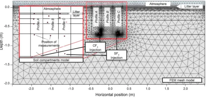
In 2009 two parallel access trenches (0.8 m depth, 1.2 m length, 0.5 m width) were dug with a separation of 2 m. Holes for gas sampling tubes were drilled through the soil between the trenches (Goffin et al., 2014; Goffin et al., 2015; Parent et al., 2013). A 1.5 m long gas-permeable sampling tube (Accurel PPV8/2, Membrana, Wuppertal, Germany) was installed into each of these holes and the trenches were refilled. The nominal depths of the tubes were 0, 0.08, 0.17, 0.35, and 0.68 m, with three replicates of each separated by 0.3 m in the direction along the trenches. Exact positions were documented and included in the gas transport modeling (Fig. 1).
The sampling tubes were connected to the surface via gas impermeable tubes. Each sampling tube was individually accessible using an electromagnetic valve system with 24 channels (Matrix, Ivrea, Italy). When a sampling tube was selected for gas analysis, sampling air circulated in a closed loop through the valve system to the analyzers and back into the respective sampling tube. Tests showed that 20 min were sufficient to equilibrate the air inside the sampling system (analyzers and sampling tubes) with the soil air. Gas concentrations were measured continuously, switching every
20 min between the positions, so that every position was measured four times per day. Daily mean values were used for soil gas modeling.
Fig. 1. 2D models of the soil profile. Gas sampling positions and spatial soil compartments are displayed in the conceptual model (zoom section).The interface between litter layer and mineral soil is set to 0 cm depth. The mesh used for Finite Element Modeling consisted of 8032 elements.
2.2.2 TRACER GAS INJECTION
The two tracer gases (CF4 and SF6) were fed separately and simultaneously into the two outer sampling tubes at the 0.68 m depth to measure soil gas diffusivity, as indicated in Fig. 2a and b (middle tube not shown), with CF4 in the left tube and SF6 in the right. The tracer gas concentrations at the respective injection positions were not used, since they were affected by the additional diffusive resistance of the sampling tube. The tracer gases can be considered as inert and their solubility in water is low. They were fed in continuously at a constant rate using a peristaltic pump (Ismatec IPN, IDEX Health & Science GmbH, Wertheim, Germany), so that after a certain time a steady state could be assumed for their transport. The injection rates were checked automatically every 6 h by bypassing each gas into a reservoir for 10 min and monitoring the increase in gas concentration (Laemmel et al., 2017). The pump rate was reduced to a minimum (< 0.05 ml min-1) by using pure CF
4 and SF6. The flow of soil air through the profile induced by the injection was negligible compared to the associated diffusion rates (Laemmel et al., 2017; van Bochove et al., 1998).
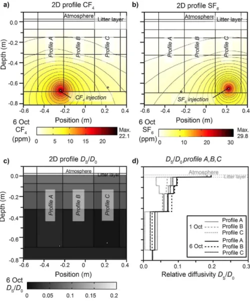
Fig. 2. Inversely modeled tracer gas concentrations and DS/ D0 on Oct 6, 2014. a) Contour plot of the
2D steady-state profile of CF4. CF4 was injected at the bottom left, b) Contour plot of the 2D
steady-state profile of SF6. SF6 was injected at the bottom right, c) The 2D DS/D0 profile showed a higher DS/D0
in the topsoil < 0.3 m depth and highest values in the litter layer, d) While the topsoil was drying from Oct 1-6, DS/ D0 in the topsoil increased. Horizontal patterns, i.e. differences between Profile A, B and C
persisted.
2.2.3 GAS ANALYSIS
The gas concentrations were measured simultaneously in the field for CO2 and CH4 using a GreenHouseGas Analyzer Ultraportable (Los Gatos Research Inc., Mountain View, US) and for N2O, CF4 and SF6 using a photoacoustic field gas monitor (Innova 1416, Lumasense, Ballerup, DK). The moisture content of the sampled air was conditioned using a dew point controller set to 8 °C. The stabilization of the water vapor allowed for a high N2O measurement precision with the photoacoustic gas monitor that was checked against a gas chromatograph in the laboratory prior to the field sampling. Accuracy was 1% of the reading for both field devices and all gases. Precision (standard deviation) was 2 ppb for CH4 and N2O, 300 ppb for CO2, < 1 ppb for CF4 and SF6. The time constant of the analyzers was < 1 min. The gas analyzers were stored in an air-conditioned cabinet as the accuracy of both devices would have been affected by temperature changes.
2.2.4 CHAMBER MEASUREMENTS
Soil-atmosphere fluxes of all analyzed gases were measured at the last day of the field campaign around noon using a non-steady-state chamber (Maier et al., 2017). Nine steel collars (diameter 15.8 cm, height 17 cm) were installed the day before the measurement. The mobile chamber lid was equipped with a small fan and a vent. Chambers were closed for 15 minutes and air was circulated between the chambers and the gas analysis system described above. Insertion depth of the collars was 2-4 cm and was considered for the calculation of the respective chamber volume. The effective chamber volume was increased by the internal volume of the gas analysis system. Flux calculations were performed using linear regressions versus time of the gas concentration changes of CO2 and CH4 (over the first 5 min) and CF4, SF6, and N2O for the full 15 min (Levy et al., 2011). Flux measurements that yielded regressions with P values > 0.05 were set to zero flux.
2.2.5 ANCILLARY MEASUREMENTS
Soil water content was monitored by averaging two horizontally installed probes per depth at 0.07 m and 0.24 m depth (ThetaProbe ML1, Delta-T Devices, Cambridge, UK). Air and soil temperature were routinely monitored using PT100 type sensors. A Vaisala PTB100 pressure sensor was used to measure barometric pressure (Vaisala Oy, Helsinki, Finland). Further meteorological data such as precipitation, relative humidity and wind speed were also measured (Hoist et al., 2008).
Soil physical data were available from earlier studies (Maier et al., 2012). In total more than 60 soil cores of 200 cm3 volume (height 5 cm) were taken at different sampling depths down to 0.9 m when the gas sampling tubes were installed (Maier et al., 2012). The porosity of the samples was determined by vacuum pycnometry. Soil gas diffusivity was measured for each core using a nonstationary one-chamber method (Maier et al., 2010). Diffusivity measurements were repeated at different soil moisture levels to obtain site and depth specific diffusivity functions (Maier et al., 2012). The soil samples were saturated with water and placed in a filter bed that allowed applying defined water potentials (see Maier et al., 2010).
2.3 GAS TRANSPORT USING FINITE ELEMENT MODELING
2.3.1 BACKGROUND: 1D GAS TRANSPORT MODELING
In a 1D soil profile, the diffusive gas flux (F, mol m-2 s-1) can be determined from Ficḱs law based on gas concentration gradients and soil gas diffusivity using Eq. (1).
where DS (m2 s-1 ) is the effective gas diffusion coefficient of the respective gas species in the soil, ρa
(mol m-3) is the air molar density, C (mol mol-1) is the gas concentration, and z (m) is the position. D
S
depends on the properties of the diffusing gas (diffusivity in free air D0 m2 s-1) and the structure of the air filled pores, that is often addressed as tortuosity (Werner et al., 2004). Tortuosity and volume of the air-filled pores depend on the total pore volume and the soil moisture. D0 is affected by air pressure and temperature (Massman, 1998). Since diffusivity in the gas phase is orders of magnitude largeer than that in the aqueous phase (Wilhelm et al., 1977), diffusion within soil pore water can be neglected in unsaturated soils (Jassal et al., 2004).
2.3.2 2D GAS TRANSPORT MODELING USING FINITE ELEMENT MODELING
To facilitate and extend the gradient method we used Finite Element Modeling (FEM) to model soil gas transport and production in 2D using the COMSOL Multiphysics pde solver (Version 5.2 COMSOL Inc., Burlington, Massachusetts, US). Molecular gas diffusion was assumed to be the only transport mechanism in the soil. 2D gas transport in the soil was described using
where DSi (m2 s-1) is the 2D effective soil gas diffusion coefficient tensor of gas species i in the soil, in
which the horizontal and vertical directions are linked by an anisotropy factor, and Ci (mol mol-1) is the gas concentration of gas species i. The relative soil gas diffusivity DS/D0, which is independent of gas species, was used to calculate (DSi) by multiplying by D0i (cm2 s-1), the D0 of gas species i. D0i is 0.21 cm2 s-1 for CH
4, 0.15 cm2 s-1 for CO2, 0.09 cm2 s-1 for SF6 (Fuller et al., 1966), 0.14 cm2 s_1 for N2O (Marrero and Mason, 1972), and 0.12 cm2 s-1 for CF
4 (Raw and Raw, 1976) at standard conditions. These D0i were modified for changes in barometric pressure and temperature according to Massman (1998).
During the field measurements, soil gas concentrations changed slowly day to day. Test runs with time dependent modeling showed that a steady state was reached within 6-10 h. Since we used daily mean values we assumed steady state diffusion, which simplified the gas budget equations to
where P i (mol m-3 s-1) represents the production rate density of the gas species i. The tracer gases were inert and diffused through the soil matrix without being produced or consumed except for their constant injection at isolated points in the profile (P i equals a point source). Time dependent modeling would be required in case of fast changes of soil gas concentrations, e.g., after rain, or strong wind events (Maier et al., 2010) or large changes in barometric pressure that can induce advective gas transport in the soil.
2.3.3 TRANSPORT AND PRODUCTION MODELING OF THE FIELD STUDY
The field study gas transport was modeled in 2D in a sufficiently large domain (Fig. 1, width 5 m, depth 2 m). The domain was split into large homogeneous compartments that formed three central profiles (A, B, C; see Fig. 1) and side profiles to the left and right. The model included a thin litter layer (0-0.02 m) and an atmospheric layer. The gas sampling locations were more or less in the center of the soil compartments (Fig. 1). The upper boundary of the atmospheric layer was set to the measured atmospheric gas concentrations as Dirichlet boundary condition, and acts therefore as sink and source for the gases. The atmosphere was assumed to be well mixed and the effective diffusivity was set to 10 D0i. The sides and the bottom of the modeled domain were impermeable (Neumann boundary condition). The width of the model was stepwise incremented until no effect on the tracer gas distribution in the entire profile was observed, to ensure that the dimension of the modeled area did not affect the modeling outcome within the profiles A, B and C. The tracer gases were injected at 0.68 m (CF4, left) and 0.64 m (SF6, right) depth. A physically optimized mesh with 8032 elements was automatically generated by the software and used for the modeling.
2.3.4 INVERSE MODELING
2D profiles of DS/D0 and P i were derived by two successive inverse modeling runs, respectively. Each soil compartment in Fig. 1 was assumed to be homogeneous and assigned an independent value for DS/ D0, PCO2, PCH4 and PN20at the beginning. Gas specific production rates (Pi) and DS/D0 values were inversely modeled for each of the soil and litter compartments of profile A, B and C down to a depth of -0.7 m. Pi and D
S/D0 of the wide compartments to the left and right of the central profiles were set to the mean of the respective values of profile A-C at the respective depth. Anisotropy of diffusivity (different vertical and horizontal values for DS) was also used as a fitting
parameter since gas transport in soil cannot be considered isotropic (Kühne et al., 2012). The values for the fitting parameters were obtained by inverse modeling such that the objective function minimized the differences between modeled and measured concentrations. For this we used Leven-berg-Marquardt and SNOPT (Sparse Nonlinear Optimizer) algorithms.
To avoid arbitrary results, a special penalty function was used for each fitting parameter, so that the optimization algorithm minimized the sum of the penalty function and the objective function. It consisted of the sum of squares of the difference between neighboring compartments for the variable to be optimized, e.g, the penalty function for PCH4, (PFCH4) is given by
where represents two horizontally neighboring compartments, and
two vertical neighbors. The weight of the penalty function was adjusted individually for the vertical and horizontal direction and was adapted for each fit parameter (DS/D0 and Pi), to account for the different orders of concentrations and P i. For PCO2 and PCH4 the penalization for the horizontal differences was 10 and 2 times stronger than for the vertical direction, respectively, since we expected dominating vertical gradients. For PN2O the same penalization was used for the horizontal and vertical direction. The penalty function for DS/D0 was 4 times stronger for the horizontal direction since we expected the vertical variability to be naturally higher. The penalization of differences between litter layer and mineral soil was reduced (by a factor of 0.01) to allow large jumps in DS/D0 between these layers. The penalty functions remained unchanged for all days modeled. Daily mean values of the gas concentrations were used. The quality of fit between measured (input) and modeled data was evaluated with the standardized root-mean-square error (SRMSE), normalized by dividing by the minimum to maximum range.
Two consecutive inverse modeling steps were used. First, DS/D0 values in all soil compartments and the anisotropy factor were determined using the injection rates and profile measurements of both tracer gases (SF6, CF4) simultaneously. Next the PCH4, PCO2, and PN2O values in all soil compartments were determined using the DS/D0 compartment values and the CO2, N2O, and CH4 profile measurements.
Fig. 3. a) Comparison of known ("forward") and inversely modeled DS/D0 values. Synthetic tracer gas
concentration were modeled forward for two known 2D DS/D0 profiles, and then used to inversely
model 2D DS/D0 profiles again, b) Modeled vs measured SF6 and CF4 concentrations showed good
agreement and low Standardized Root Mean Square Errors (SRMSE). c) Comparison of inversely FEM modeled DS/D0 profiles and DS/D0 valuesderived from diffusivity model (Ma = ; Mo 00 = ; Mo 97 = ; M-Q =
). Boxplots are slightly shifted in depth for better visibility. Inversely modeled DS/D0 data include 3
Table 1. Relative errors (Rel. er)., mean (and standard deviation) between known ("forward") and inversely modeled DS/D0 and Pi values per depth of two simulated profiles, (e.g. Rel. er. Pi = Pi (inverse)/Pi(forward)-1).
Depth (m) Rel. er.
(%) DS/D0 Rel. er. P CH4 (%) Rel. er. P CO2 (%) Rel. er. P N2O (%) 0.01 -4(5) -9(34) -2(2) 6(39) -0.04 1 (3) 1 (2) 0(3) -2(17) -0.12 -1 (1) -4(8) 4(6) -2(9) -0.25 0(2) 7(17) -2(14) 3(15) -0.6 0(0) - 26 (68) 4(21) 6(39)
2.3.5 SENSITIVITY AND VALIDATION
To evaluate the sensitivity of the FEM approach we used two approaches: (a) To assess the accuracy and sensitivity of the inverse modeling procedure we synthetically generated data sets of soil gas concentrations at the gas sampling locations with Eqs. (1) and (2) using known 2D profiles of DS/D0 and P i, and then used these concentrations as inputs to the inversion algorithms described above to recalculate DS/D0 and P i, as done for 1D by Novak (2007). Differences between the known input data from the forward model and the inversely modeled 2D profile of DS/D0 and P i were attributed to the inverse modeling procedure. To obtain realistic parameter sets, we used 2D profiles from our model results to generate the synthetic data sets. The evaluations were done in two steps. First the gas concentrations for the synthetic tracer study were simulated. The simulated tracer gas concentrations at the gas sampling locations were used to determine DS/D0 of the soil compartments by inverse modeling which were then compared to the known assumed
DS/D0 values. Next these inverted DS/D0 values were used in a forward determination of gas concentrations at the gas sampling locations with known assumed PCH4, PCO2
, and PN2O followed by
inversion to recalculate the respective Pi in the soil compartments, (b) To consider the sensitivity to measurement errors in the input data we used the daily minimum and maximum soil gas concentrations in addition to the daily mean for the inverse modeling.
To validate the 2D gas transport modeling we compared the modeled soil-atmosphere fluxes with those measured by the field chambers. Modeled 2D profiles of DS/D0 were also compared to values derived from well-known soil diffusivity models.
Table 2. Standardized root mean square error (SRMSE) between measured and inversely modeled gas concentrations (SF6, CF4, CO2, CH4, N2O) on Oct 1 and Oct 6, 2014.
Date SRMSE CF4 SRMSE SF6 SRMSE CH4 SRMSE CO2 SRMSE N2O
Oct 1, 2014 0.0495 0.0176 0.0141 0.0305 0.0451
Table 3. Comparison of mean values (and standard deviation) of soil-atmosphere fluxes of the tracer gases SF6 CF4, and the greenhouse gases CO2, CH4, and N2O based on estimations using chamber
measurements and modeled profile fluxes using COMSOL.).
Method
(unit) Date CF4 (nmol m
-2 s) SF
6 (nmol m-2 s) CH4 (nmol m-2 s) CO2 (µmol m-2 s) N2O (nmol m-2 s)
COMSOL Oct 1, 2014 0.123 (0.104) 0.073 (0.043) -1.03 (0.186) 1.68 (0.22) -0.061 (0.03) COMSOL Oct 7, 2014 0.140 (0.106) 0.095 (0.075) -1.29 (0.049) 1.92 (0.056) -0.032 (0.010) Chamber Oct 7, 2014 0.125 (0.105) 0.109 (0.048 -1.52 (0.195) 3.07 (0.459) -0.053 (0.080)
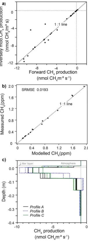
Fig. 4. Inversely modeled CH4 concentrations and PCH4 a) 2D CH4 profile on Oct 6, 2014. CH4
concentrations decreased with soil depth, b) The pattern of the CH4 Profile A, B and C persisted and
shifted to higher CH4 values from Oct 1 to Oct 6, 2014. c) The 2D PCH4 profile showed a high CH4
consumption in the Ah horizon down to 0.17 m depth, d) Maximum CH4 uptake shifted from the litter
2.3.6 REFERENCE VALUES FROM DIFFUSIVITY MODELS
A common way to express the soil gas diffusivity is to use the relative soil gas diffusivity DS/D0 that is independent of the diffusing gas.
Reference values of the relative soil gas diffusivity DS/D0 were calculated using four well-known diffusivity models from the literature.
1) Ma: DS/D0 = a∙εb with parameters a = 1.50 and b = 2.74 determined at the same site (Maier et al., 2012).
2) Mo 00: DS/D0 = ε2.5∙ϕ-1 (Moldrup et al., 2000). 3) Mo 97: DS/D0 = 0.66∙ε3∙ϕ-3 (Moldrup et al., 1997). 4) M-Q: DS/D0 = ε3.33∙ϕ-2 (Millington and Quirk, 1961).
In these relationships ϕ, (m3 m) is the porosity and ε (m3 m -3) is the filled pore volume. The air-filled pore-volume was calculated as the difference between porosity and volumetric soil water content. Reference DS/D0 values were calculated for both soil moisture measurements at each depth as an indication of variability.
2.4 FIELD MEASUREMENTS
Soil gas concentrations were monitored from Oct 1 to Oct 7, 2014. There was no rain during the field measurements and the mean soil moisture content decreased from 36.3 to 32.8 % in the topsoil (loamy silt) and remained stable at 30 % at 0.24 m depth (loamy sand) (see online supplement). Daily mean air temperature remained stable at 13.0 °C, mean soil temperatures at 0.03, 0.1, 0.2, and 0.4 m depths ranged between 14.0 and 14.5 °C.
SF6 and CF4 were continuously injected into the soil at rates of 0.26 µmol s-1 and 0.33 µmol s-1, respectively, on Oct 1. The injection rates slowly increased during the measurement period, reaching values of 0.31 µmol s-1 and 0.41 µmol s-1, for SF
6 and CF4, respectively on Oct. 6. Chamber measurements were conducted at the end of the campaign. Reference DS/D0 estimates using the formulas above were calculated based on measured soil physical properties and soil moisture contents for Oct. 6.
Fig. 5. a) Comparison of known ("forward") and inversely modeled PCH4 values. Synthetic CH 4
concentration were modeled forward for two known 2D PCH4 profiles, and then used to inversely model
2D PCH4 profiles again, b) Modeled vs measured CH
4 concentrations showed good agreement and low
SRMSE. c) Inversely modeled PCH4 data (as shown in Fig. 4d) including 3 lines per profile that represent
3 Results and Discussion
3.1 INVERSE MODELING OF SOIL GAS DIFFUSIVITY
3.1.1 2D PROFILES OF SOIL GAS DIFFUSIVITY
Tracer gas concentrations reached 8.5 ppm SF6 and 6 ppm CF4 at the positions next to the respective injection tube (Fig. 2a and b). Maximum concentration of SF6 was higher than that of CF4 although the SF6 injection rate was lower. This was partly due to the lower D0 of SF6 compared to CF4, but also due to the spatial heterogeneity of the gas diffusivity of the soil, as seen from the fact that DS/D0 in profile C (SF6 injection) was lower than DS/D0 of profile A (CF4 injection) (Fig. 2c). Tracer gas concentrations increased towards the injection tubes, having concentric isolines (Fig. 2a and b). Tracer gas concentrations decreased slightly during the observation period although the injection rate was slightly increasing (see online supplement). This indicated increasing bulk diffusivity in the soil profile over time that can be explained by the measured decreasing soil moisture content and increasing air-filled porosity.
DS/D0 was higher in the topsoil (< 0.3 m depth) than in the deeper soil, with highest values in the litter layer (Fig. 2c and d). The 2D DS/D0 profile showed substantial horizontal differences between the topsoil compartments of up to 50%.
Soil moisture in the topsoil decreased faster than in the subsoil during the measurements. Correspondingly, DS/D0 of the litter layer and topsoil increased from Oct 1 to Oct 6, while DS/D0 changed marginally in the subsoil. The decreasing soil water content in the topsoil resulted in an increasing air-filled porosity and higher DS/D0 values.
The clear differences in DS/D0 between litter layer, topsoil and subsoil persisted for the whole measurement campaign (Fig. 2d), reflecting the large physical differences of the organic litter layer, the silty topsoil and the sand dominated subsoil. Also the relative spatial pattern persisted with profile C always having the lowest DS/D0 (Fig. 2c and d). This indicates that we have to consider relevant spatial patterns of soil aeration that persist over time, with some areas in a soil profile can
e.g. receive a better supply with atmospheric oxygen or methane, or become anaerobic when soil
moisture increases. Studies on soil monoliths showed high spatial heterogeneity in DS/D0 as a result of macro-pores like cracks and burrows that can play an important role for soil aeration (Allaire et al., 2008; Lange et al., 2009). Our results showed that we have to expect relevant and persistent 2D patterns in DS/D0 even in soils that are considered to be homogeneous as at our study site.
Including an anisotropy factor as a fit parameter in the inverse modeling yielded a better fit for the SF6 and CF4 concentrations with a lower SRMSE. The inversely modeled anisotropy factor was 1.26 (vertical DS/horizontal DS). This is close to the factor of 1.38 that was observed in a study using soil cores from a forest site and laboratory measurements (Kühne et al., 2012). We argue that both earthworms and gravity are major engineers of this effect. Earthworms preferentially burrow vertical holes while gravity destabilizes preferentially horizontal pores.
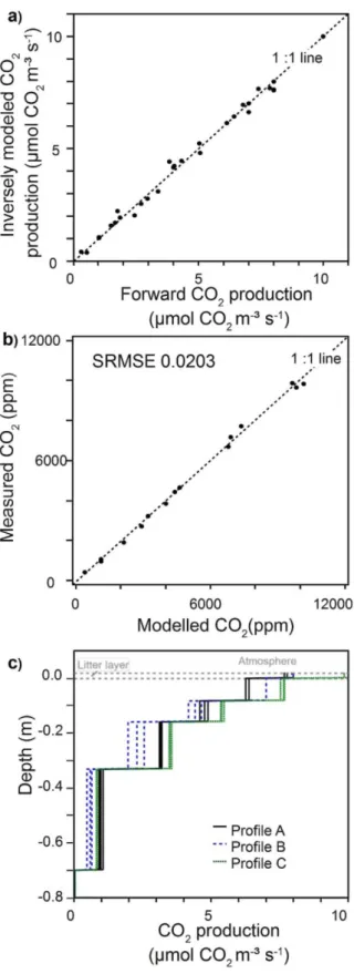
Fig. 6. Inversely modeled CO2 and PCO2 a) 2D CO2 profile on 6 Oct, 2014. b) Modeled CO2 profiles shifted
slightly towards lower CO2 concentrations from Oct 1 to Oct 6. c) The 2D PCO2 profile showed the
highest CO2 production in the litter layer and top soil, d) From Oct l to 6, Profile A, B, and C showed a
slight decrease in PCO2 in the litter layer and increase in the mineral soil.
3.1.2 UNCERTAINTY IN THE MODELED DIFFUSIVITY PROFILE AND COMPARISON WITH D
S/D
0MODELS
The sensitivity test using known ("forward") and inversely modeled 2D diffusivity profiles showed good agreement between the DS/D0 values (Fig. 3a). Inversely modeled DS/D0 values in the litter layer underestimated known values by at most 4% on average (Table 1). The high DS/D0 values deviating from the 1:1 line represent the litter layer in profile B. The inverse modeling procedure seemed to best fit DS/D0 values at greater depths.
Good agreement between measured and modeled SF6 and CF4 concentrations (Fig. 3b) was achieved by inverse modeling of the 2D DS/D0 profiles, with standardized root mean square errors SRMSE < 0.05 (Table 2). Including the daily minimum and maximum soil SF6 and CF4 concentrations allowed giving a measure of uncertainty in the inversely modeled DS/D0 profiles of Oct 6 (Fig. 3c). The range between the replications of the profiles derived from the daily minimum, mean and maximum concentrations were lowest in the subsoil. We think that the FEM approach yielded sensitive estimates of the DS/D0 profile. Yet, inaccurately modeled values occurred in the litter layer, where DS/D0 values were highest, and concentration gradients were lowest.
SF6 and CF4 surface fluxes were estimated using the FEM approach and compared to chamber fluxes. Both methods showed good agreement (Table 3) supporting the concept of the FEM
approach. FEM derived DS/D0 estimates were compared to values derived from diffusivity models that were calculated for both soil moisture measurements at each depth (Fig. 3c). The DS/D0 values derived from diffusivity models and from FEM showed the same decrease with depth. DS/D0 derived from the Ma and Mo 00 models are similar, but they changed their order with depth because the Mo 00 model uses an additional parameter. Differences in DS/D0 obtained from the different diffusivity models were large. The M-Q and Mo 97 diffusivity models were closest to the FEM derived profiles. Surprisingly, the on-site calibrated Ma model didn't perform as well as the M-Q and Mo 97 models, probably due to plot scale variability in texture and soil structure at this site.
All (SF6, CF4, CO2, CH4, N2O) chamber derived fluxes agreed well with the fluxes estimates from the 2D FEM approach (Table 3), which are largely dependent on an accurate DS/D0 assessment. Hence, we think that the M-Q and FEM derived DS/D0 estimates are most realistic. This also means that estimating the surface flux using the gradient method (Maier and Schack-Kirchner, 2014) yielded better results for the in situ determined DS/D0 than it would for the Ds/D0 derived from diffusivity
models. The large differences in Ds/D0 values between the diffusivity models demonstrate the
difficulty of choosing the best model a priori, and the need to validate a chosen model by measurements on local samples.
Fig. 7. a) Comparison of known ("forward") and inversely modeled pco2 values. Synthetic CO 2
concentrations were modeled forward for two known 2D pco2 profiles, and then used to inversely
model 2D pco2 profiles again, b) Modeled vs measured C0
2 concentrations showed good agreement
and low SRMSE. c) Inversely modeled pco2 data (as shown in Fig. 6d) including 3 lines per profile that
3.2 INVERSE MODELING OF PRODUCTION AND CONSUMPTION OF CH
4, CO
2AND
N
2O
3.2.1 CONCENTRATIONS AND CONSUMPTION OF CH
4IN THE SOIL PROFILE
Chamber measurements and gas transport modeling showed that the soil at Hartheim was a CH4 sink during the study period (Fig. 4, Table 3), ranging from -1.52 to -1.03 nmol m-2 s-1. Soil CH
4 concentrations slowly increased over time, and the spatial pattern between the different sampling positions persisted (see online supplement). Soil CH4 was always below ambient concentrations and decreased with depth, indicating CH4 consumption (negative production) throughout the soil profile. Concentrations < 0.2 ppm were reached at depth > 0.5 m (Fig. 4a). CH4 concentrations between 0.15 and 0.4 m depth were higher in profile B than in the other profiles (Fig. 4b).
FEM showed that more than 85% of the CH4 consumption occurred in the top 0.2 m of the soil where the atmospheric CH4 supply was the best, reaching -10.6 nmolm-3 s-1 (Fig 4c and d). The layers below received less CH4 and CH4 consumption rates were lower. A similar decrease in CH4 consumption with depth was observed in all profiles, yet horizontal differences between the profiles were substantial (Fig. 4c and d). Profile B showed the highest CH4 consumption in the topsoil, while the CH4 consumption in the subsoil was the lowest (Fig. 4d). The observed low CH4 consumption does not necessarily mean that the microbial composition in this compartment was different; it could also result from the reduced supply due to CH4 consumption in the soil above. CH4 concentrations increased slowly at all measurements locations over time, e.g. at 0.17 m depth from 0.40 to 0.49 ppm (see online supplement). Inverse modeling of PCH4 showed that the higher CH4 concentrations resulted from the higher diffusivity and - counter-intuitively - a higher CH4 consumption. The higher diffusivity led to a better supply with CH4 stimulating a higher methanotrophic activity, so that deeper layers became more active. Maximum methanotrophic activity shifted from the litter layer (Oct 1) down into the topsoil (Oct 6) over time (Fig. 4d), probably because the litter layer (including mineral compounds) became too dry. Other studies (Adamsen and King, 1993; Karbin et al., 2016; Niklaus et al., 2016; Rosenkranz et al., 2006;) also showed that CH4 consumption is highest in the top centimeters of the mineral soil and that a decreasing soil water content is often associated with a higher CH4 consumption (Borken and Beese, 2006; Butterbach-Bahl et al., 2002; Hartmann et al., 2011). Stiehl-Braun et al. (2011) observed that the most active zone of CH4 consumption shifted downward within the soil profile during a drought. Although we were far from experiencing a drought, a similar shift of CH4 consumption was observed. This could be explained by a better supply of atmospheric CH4 to deeper layers due to increasing soil gas diffusivity. Our observation supports the hypothesis that diffusion of atmospheric CH4 into the soil is the main limiting factor for CH4 oxidation in upland forest soils (Ball et al., 1997; Smith et al., 2003).
CH4 can be consumed and produced at the same time within a soil profile (Butterbach-Bahl et al., 2002) and this possibly occurred in our soil. It is important to note that all PCH4 rates are net rates and that this can always include CH4 production, e.g. in oxygen depleted zones within aggregates (Kuzyakov and Blagodatskaya, 2015). Approaches using the isotopic signatures of CH4 can help answer questions of the partitioning between sink and source (Fischer and von Hedin, 2002), and would further improve the spatial mapping of methanotrophic and methanogenic activity in the soil.
3.2.2 UNCERTAINTY IN THE MODELED CH
4CONSUMPTION PROFILE
A sensitivity test using known ("forward") and inversely modeled 2D PCH4 profiles showed generally good agreement between the PCH4 values (Fig. 5a). Yet, inverse modeling underestimated mean PCH4 in the litter layer by 9% (Table 1) resulting from a substantial underestimation in the litter layer in the profile B (2 points left of the 1:1 line in Fig. 5.a). The relative error was also large in the subsoil, as a result of PCH4 values close to zero; absolute PCH4 errors were small in this case.
Good agreement between measured and modeled CH4 concentrations (Fig. 5b) was achieved by inverse modeling of the CH4 profiles, with SRMSE < 0.02 (Table 2). Chamber measurements and FEM derived soil-atmosphere CH4 fluxes showed good agreement on Oct 7 (Table 3). Including daily minimum and maximum soil CH4 concentrations in the inverse modeling on Oct 6 confirmed the vertical pattern in the PCH4 and the horizontal differences between profiles A-C (Fig. 5c). The Min-Max PCH4 values showed a wider range in profile B in the upper soil, this can be interpreted as a higher uncertainty.
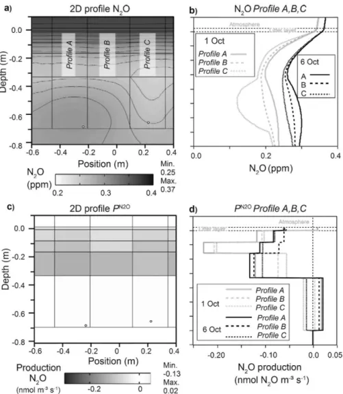
Fig. 8. Inversely modeled N2O and PN2O profiles, a) 2D profile of N2O concentrations on Oct 6. b) N2O
concentration profiles had a minimum around 0.3 m depth. The atmospheric N2O concentration
increased slightly by 0.015 ppm from Oct 1-6 and the whole gas profile was shifted from Oct 1 to 6. c) On Oct 6, the topsoil was taking up N2O and the subsoil tended to N2O production on Oct 6. d) The
pronounced N2O uptake in 0.07-0.15 m depth on Oct 1 leveled out by Oct 6.The 2D PN2O profile changed
3.2.3 CONCENTRATIONS AND PRODUCTION OF CO
2IN THE SOI PROFILE
Measurements and modeling showed that the soil-atmosphere flux of CO2 at Hartheim represented the largest GHG flux during our study (Table 3), ranging from 1.68 to 3.07 µmol m-2 s-1. Soil CO
2 concentrations slightly decreased with time (see online supplement). CO2 concentrations increased with depth, reaching > 10000 ppm (Fig 6a and b). Most of the CO2 was produced in the top 0.3 m (Fig. 6c and d), which is also the most intensively rooted zone (Goffin et al., 2014). PCO2 reached 10 µmol m-3 s-1 in the litter layer (Fig. 6c and d). The subsoil > 0.35 m depth also contributed to the CO2 production. The modeled PCO2 profiles agreed well with that found by Goffin et al. (2014) at the same site and other sites where most of the soil CO2 originates from the upper soil layers (Davidson et al., 2006; Novak, 2007).
Horizontal differences in CO2 and PCO2 were observed (Fig. 6), but they were less pronounced than differences in DS/D0 or PCH4. We conclude that soil respiration is not affected by soil gas diffusivity as long as the soil is well aerated, but that soil respiration rather depends on the homogenous distribution of roots and organic carbon at this site.
Soil CO2 efflux (= sum of PCO2 per area) increased during the monitoring period by 14% (Fig. 6d, Table 3), despite the fact that soil CO2 concentrations slightly decreased (from 10500 ppm to 9800 ppm at 0.65 m depth, see online supplement). This might seem counterintuitive at the first glance, but can be easily explained by the increase in Ds/D0 (Fig 2d). The increase in total soil respiration
from Oct 1 to Oct 6 was due to the increase of PCO2 in the mineral soil while PCO2 in the litter layer decreased. This decrease probably resulted from litter drying and becoming biologically less active, as it was also observed for PCH4
3.2.4 UNCERTAINTY IN THE MODELED CO
2PRODUCTION PROFILE
Known ("forward") and inversely modeled 2D PCO2 profiles showed good agreement (Fig. 7a). While the mean PCO2 values agreed well in all depths (Table 1), the standard deviation increased with depth, indicating that the horizontal variability was not correctly reflected. Since PCO2 values were small in the subsoil, absolute PCO2 errors were still small.
Good agreement between measured and modeled CO2 concentrations (Fig 7b) was achieved by inverse modeling of the CO2 and PCO2 profiles, with SRMSE < 0.04 (Table 2). Including daily minimum and maximum soil CO2 concentrations Oct 6 yielded narrow minimum-maximum ranges for PCO2 i∏ profile A&C, and slightly larger uncertainty ranges for profile B (Fig 7c). These uncertainty ranges were small compared to the changes in the 2D PCO2 profiles between Oct 1-6. The FEM derived CO
2 flux was 37% lower than the FEM derived flux (Table 3). This can be attributed to CO2 produced in the litter layer that hardly affects the CO2 concentrations. As a result, the uncertainty of PCO2 estimation in the litter layer was higher and lead to a deviation between gradient based flux estimations and chamber measurements (Davidson and Trumbore, 1995; Maier and Schack-Kirchner, 2014). Studies comparing chamber method and gradient flux method yielded better agreement when the soil surface was dry and inactive (Myklebust et al., 2008; Tang et al., 2003; Tang et al., 2005; Vargas and Allen, 2008). The litter layer was still moist in our study. Davidson and Trumbore (1995) used the flux difference between gradient flux method and chamber measurements to derive the litter borne soil respiration, in our case this would be 37% of the chamber measured efflux. This means, that the PCO2 in the litter layer was probably much higher than estimated by the FEM.
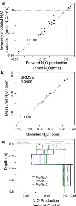
Fig. 9. a) Comparison of known ("forward") and inversely modeled PN2O values. Synthetic N 2O
concentration were modeled forward for two known 2D PN2O profiles, and then used to inversely
model 2D PN2O profiles again, b) Modeled vs measured N
2O concentrations showed good agreement
and low SRMSE. c) Inversely modeled PN2O data (as shown in Fig. 6d) including 3 lines per profile
3.2.5 CONCENTRATIONS AND CONSUMPTION AND PRODUCTION OF N
2O IN THE SOIL
PROFILE
Chamber measurements and the FEM approach showed that the soil was a sink for N2O during our study. Soil-atmosphere fluxes ranged from -0.06 to -0.03 nmol m-2 s-1 (Table 3), agreeing with N
2O uptake observed at other sites (Butterbach-Bahl et al., 2002; Chapuis-Lardy et al., 2007; Rosenkranz et al., 2006). Soil N2O concentrations were always below ambient concentrations and decreased with depth (Fig. 8a and b), reaching 0.16 ppm at 0.65m depth. N2O concentrations fluctuated on a diurnal scale, but daily mean values showed stable temporal trends (online supplement). The N2O concentrations in the subsoil were more scattered than in the topsoil. Below 0.3 m depth, the 2D N2O profiles showed horizontal concentration gradients as high as the vertical gradients below 0.3 m depth (Fig. 8a and b).
Most of the N2O consumption occurred in the topsoil reaching -0.23 nmol m-3s-1 (Fig 8c and d). Subsoil (> 0.35 m depth) N2O fluxes were an order of magnitude smaller than the soil-atmosphere flux. Modeling yielded small negative and positive PN2O values, and horizontal fluxes as large as vertical fluxes. The 2D profiles of PN2O were more variable than CO
2 or CH4. Soils can be sinks but also sources for atmospheric N2O, depending on the prevailing process, consumption or production of N2O (Chapuis-Lardy et al., 2007).
3.2.6 UNCERTAINTY IN THE MODELED N
2O CONSUMPTION AND PRODUCTION PROFILE
A sensitivity test using known ("forward") and inversely modeled 2D PN2O profiles showed that the mean PN2O values agreed reasonably (Table 1, Fig. 9a). Standard deviations were high, indicating that the horizontal variability was not properly reflected. Nevertheless, good agreement between measured and modeled N2O concentrations (Fig 9b) was achieved by inverse modeling of the N2O and PN2O profiles, with SRMSE < 0.05 (Table 2). Including daily minimum and maximum soil N2O concentrations in the inverse modeling resulted in wide minimum-maximum ranges of PN2O (Fig. 9c), due to the scattering of the N2O concentrations on the diurnal scale.
Chamber measurements and FEM derived soil-atmosphere fluxes were in the same order of magnitude, but mean values seemed to deviate. The observed difference in the mean N2O flux, however, was not significant since the chamber measurements had a very high variability (Table 2). This variability probably results from N2O consumption and production at the aggregate scale at hotspots (Chapuis-Lardy et al., 2007; Davidson and Verchot, 2000; Kuzyakov and Blagodatskaya, 2015) that can be expected in the microbial highly active moist litter layer. We have to consider that both N2O production and N2O consumption may occur simultaneously at different microsites next to each other (Conrad, 1996; Smith et al., 2003). The scale of the FEM model compartments was much larger than these microsites. Nevertheless, our 2D mapping approach can indicate the effective net process within the analyzed compartment.
The sensitivity tests showed that the inverse modeling step can introduce artifacts and have an important impact on the modeled 2D profiles. Using daily mean concentrations of N2O reduced most of the scattering in the data. Knowing this, N2O data have to be interpreted carefully.
3.3 MODELING ASPECTS
Simple sensitivity tests showed that the FEM approach could produce reasonable results for the 2D profiles of DS/D0: PCO2 and PCH4.
Higher uncertainty has to be expected in the litter layer, and generally when PN2O is modeled. This effect can be attributed to the small concentration gradients that were found in the litter layer for all gases, and especially in the N2O soil profile where fluxes and gradients were minimal.
Additionally, the design of the physical model affects the results obtained, e.g. choosing several smaller or few larger soil compartments, or using discrete PCO2 values for the soil compartments or a mathematical function describing the whole PCO2 profile (Maier and Schack-Kirchner, 2014; Novak, 2007). Inverse modeling questions may be ill posed, and a penalty function required. Choosing the right penalty function is essential, since it favors certain structures in the optimized parameter. Both steps, the choice of the physical model and the penalty function affect the results of the modeling and have to be chosen carefully. However, leaving the physical model and the penalty function unchanged for all days modeled allowed us to reliably interpret the changes over the days.
3.4 FUTURE APPLICATIONS
Soil gas diffusivity needs to be known to interpret soil gas concentrations. Unfortunately, it is not possible to know a priori which of the existing diffusivity models fits a given soil best. Monitoring soil gas diffusivity over a longer time with changing soil water contents would allow deriving more realistic diffusivity models.
Our approach allowed analyzing spatial patterns of soil gas diffusivity and the production of GHG in the soil, and monitoring the temporal dynamics of these. Modeling soil gas transport in 3D should be a next step since most soils exhibit complex structures such as compacted zones, cracks, mouse holes or large roots. Combining the FEM approach with methods using isotopically labeled CO2 (Hagedorn et al., 2016; Klein et al., 2016) would allow further investigation of the below ground allocation of carbon. Combining the FEM approach with methods that are able to map methanotrophic activity in the soil (Niklaus et al., 2016) would allow for a better understanding of methane consumption in soil.
4 Conclusions
We conclude that our new method represents a valuable tool for analyzing spatial and temporal variability of gas fluxes and production at a soil profile scale and that it will allow novel insights into the dynamics of soil gases. The method was able to produce reliable results if sufficiently strong gas concentration gradients occur. Further development must include the 3D investigation of soil gas processes in more complex soils.
ACKNOWLEDGEMENTS
We would like to thank Prof. Schmid, Center for Technomathematics, Bremen University, for their assistance with FEM, N. Koele for proofreading, and the German Research Foundation (DFG) for funding this research project (Ma- 5826/2-1). We also would like to thank the anonymous reviewer and M. Novak for their substantial contribution and constructive comments.
APPENDIX A. SUPPLEMENTARY DATA
Supplementary data associated with this article can be found, in the online version, at http://dx.doi.Org/10.1016/j.agrformet.2017.07.008.
References
Adamsen, A., King, G.M., 1993. Methane Consumption in Temperate and Subarctic Forest Soils: Rates, Vertical Zonation, and Responses to Water and Nitrogen. Appl. Environ. Microbiol. 59 (2), 485-490.
Allaire, S.E., Lafond, J.A., Cabral, A.R., Lange, S.F., 2008. Measurement of gas diffusionthrough soils: comparison of laboratory methods. J. Environ. Monit. 10 (11),1326-1336.
Ball, B., Smith, K.A., Klemedtsson, L., Brumme, R., Sitaula, B.K., Hansen, S., Priemé, A., MacDonald, J., Horgan, G.W., 1997. The influence of soil gas transport properties on methane oxidation in a selection of northern European soils. J. Geophys. Res. 102 (D19), 23309.
Borken, W., Beese, F., 2006. Methane and nitrous oxide fluxes of soils in pure and mixed stands of European beech and Norway spruce. Eur. J. Soil Sci. 57 (5), 617-625.
Butterbach-Bahl, K., Breuer, L., Gasche, R., Willibald, G., Papen, H., 2002. Exchange of trace gases between soils and the atmosphere in Scots pine forest ecosystems of the northeastern German lowlands. For. Ecol. Manage. 167 (1-3), 123-134.
Chapuis-Lardy, L., Wrage, N., Metay, A., Chotte, J.-L., Bernoux, M., 2007. Soils, a sink for N2O? A review. Global Change Biol. 13 (1), 1-17.
Conrad, R., 1996. Soil microorganisms as controllers of atmospheric trace gases (H2, CO, CH 4, OCS, N2O and NO). Microbiol. Rev 60, 609-640. Davidson, E.A., Savage, K.E., Trumbore, S.E., Borken, W., 2006. Vertical partitioning of CO2 production within a temperate forest soil. Global Change Biol. 12 (6), 944-956.
Davidson, E.A., Trumbore, S.E., 1995. Gas diffusivity and production of CO2 in deep soils of the eastern Amazon. Tellus B 47 (5), 550-565.
Davidson, E.A., Verchot, L.V., 2000. Testing a Conceptual Model of Soil Emissions of Nitrous and Nitric Oxides. Global Biogeochem. Cycles 14 (4), 1035-1043.
DeJong, E., Schappert, H.J.V., 1972. Calculation of soil respiration and activity from CO2 profiles in the soil. Soil Science 113 (5), 328-333.
FAO, 2006. World reference base for soil resources 2006: A framework for international classification, correlation and communication. FAO, Rome 128 pp.
Fischer, J.C., von Hedin, L.O., 2002. Separating methane production and consumption with a field-based isotope pool dilution technique. Global Biogeochem. Cycles 16 (3) 8-1-8-13.
Fuller, E.N., Schettler, P.D., Giddings, J.C., 1966. New method for prediction of binary gas/phase diffusion coefficients. Ind. Eng. Chem. 58 (5), 18-27.
Goffin, S., Aubinet, M., Maier, M., Plain, C, Schack-Kirchner, H., Longdoz, B., 2014. Characterization of the soil CO2 production and its carbon isotope composition in forest soil layers using the flux-gradient approach. Agr. For. Met. 188, 45-57.
Goffin, S., Wylock, C, Haut, B., Maier, M., Longdoz, B., Aubinet, M., 2015. Modeling soil CO2 production and transport to investigate the intra-day variability of surface efflux and soil CO2 concentration measurements in a Scots Pine Forest (Pinus Sylvestris, L.). Plant Soil 390 (1-2), 195-211.
Hagedorn, F., Joseph, J., Peter, M., Luster, J., Pritsch, K., Geppert, U., Kerner, R., Molinier, V., Egli, S., Schaub, M., Liu, J.-F., Li, M., Sever, K., Weiler, M., Siegwolf, R.T.W., Gessler, A., Arend, M., 2016. Recovery of trees from drought depends on belowground sink control. Nature plants 2, 16111. Hartmann, A.A., Buchmann, N., Niklaus, P.A., 2011. A study of soil methane sink regulation in two grasslands exposed to drought and N fertilization. Plant Soil 342 (1-2), 265-275.
Hoist, J., Barnard, R., Brandes, E., Buchmann, N., Gessler, A., Jaeger, L., 2008. Impacts of summer water limitation on the carbon balance of a Scots pine forest in the southern upper Rhine plain. Agr. For. Met. 148 (11), 1815-1826.
Jassal, R., Black, A., Novak, M., Morgenstern, K., Nesic, Z., Gaumont-Guay, D., 2005. Relationship between soil CO2 concentrations and forest-floor CO2 effluxes. Agr. For. Met. 130 (3-4), 176-192. Jassal, R.S., Black, T.A., Drewitt, G.B., Novak, M.D., Gaumont-Guay, D., Nesic, Z., 2004. A model of the production and transport of CO2 in soil: Predicting soil CO2 concentrations and CO2 efflux from a forest floor. Agr. For. Met. 124 (3-4), 219-236.
Karbin, S., Hagedorn, F., Hiltbrunner, D., Zimmermann, S., Niklaus, P.A., 2016. Spatial micro-distribution of methanotrophic activity along a 120-year afforestation chronosequence. Plant Soil 31, 978.
Klein, T., Siegwolf, R.T.W., Korner, C, 2016. Belowground carbon trade among tall trees in a temperate forest. Science 352 (6283), 342-344.
Kuhne, A., Schack-Kirchner, H., Hildebrand, E.E., 2012. Gas diffusivity in soils compared to ideal isotropic porous media. J. Plant Nutr. Soil Sci. 175 (1), 34-45.
Kuzyakov, Y., Blagodatskaya, E., 2015. Microbial hotspots and hot moments in soil: Concept & review. Soil Biol. Biochem. 83, 184-199.
Laemmel, T., Maier, M., Schack-Kirchner, H., Lang, F., 2017. An in situ method for realtime measurement of gas transport in soil. Eur. J. Soil Sci. 68 (2), 156-166.
Lange, S.F., Allaire, S.E., Rolston, D.E., 2009. Soil-gas diffusivity in large soil monoliths. Eur. J. Soil Sci. 60 (6), 1065-1077.
Levy, P.E., Gray, A., Leeson, S.R., Gaiawyn, J., Kelly, M.P.C., Cooper, M.D.A., Dinsmore, K.J., Jones, S.K., Sheppard, L.J., 2011. Quantification of uncertainty in trace gas fluxes measured by the static chamber method. Eur. J. Soil Sci. 62 (6), 811-821.
Maier, M., Machacova, K., Lang, F., Svobodova, K., Urban, O., 2017. Combining soil and tree-stem flux measurements and soil gas profiles to understand CH4 pathways in Fagus sylvatica forests. J. Plant Nutr. Soil Sci. 21, 53.
Maier, M., Schack-Kirchner, H., 2014. Using the gradient method to determine soil gas flux: A review. Agr. For. Met. 192-193, 78-95.
Maier, M., Schack-Kirchner, H., Aubinet, M., Goffin, S., Longdoz, B., Parent, F., 2012. Turbulence Effect on Gas Transport in Three Contrasting Forest Soils. Soil Sci. Soc. Am. J. 76 (5), 1518.
Maier, M., Schack-Kirchner, H., Hildebrand, E.E., Hoist, J., 2010. Pore-space CO2 dynamics in a deep, well-aerated soil. Eur. J. Soil Sci. 61 (6), 877-887.
Marrero, T.R., Mason, E.A., 1972. Gaseous Diffusion Coefficients. J. Phys. Chem. Ref. Data 1 (1), 3. Massman, W.J., 1998. A review of the molecular diffusivities of H2O, CO2, CH4, CO,O3, SO2, NH3, N2O, NO, and NO2 in air, O2 and N2 near STP. Atmos. Environ. 32 (6), 1111-1127.
Moldrup, P., Olesen, T., Gamst, J., Schjønning, P., Yamaguchi, T., Rolston, D.E., 2000. Predicting the Gas Diffusion Coefficient in Repacked Soil. Soil Sci. Soc. Am. J. 64 (5), 1588.
Moldrup, P., Olesen, T., Rolston, D.E., Yamaguchi, T., 1997. Modeling diffusion and reaction in soils: VII. Predicting gas and ion diffusivity in undisturbed and sieved soils. Soil Sci. 162 (9), 632-640. Myklebust, M.C., Hipps, L.E., Ryel, R.J., 2008. Comparison of eddy covariance, chamber, and gradient methods of measuring soil C02 efflux in an annual semi-arid grass, Bromus tectorυm. Agr. For. Met. 148 (11), 1894-1907.
Niklaus, P.A., Le Roux, X., Poly, F., Buchmann, N., Scherer-Lorenzen, M., Weigelt, A., Barnard, R.L., 2016. Plant species diversity affects soil-atmosphere fluxes of methane and nitrous oxide. Oecologia 181 (3), 919-930.
Novak, M.D., 2007. Determination of soil carbon dioxide source-density profiles by inversion from soil-profile gas concentrations and surface flux density for diffusion-dominated transport. Agr. For. Met. 146 (3-4), 189-204.
Parent, F., Plain, C, Epron, D., Maier, M., Longdoz, B., 2013. A new method for continuously measuring the δ 13 C of soil CO
2 concentrations at different depths by laser spectrometry. Eur. J. Soil Sci. 64 (4), 516-525.
Pingintha, N., Leclerc, M.Y., Beasley Jr., J.P., Zhang, G., Senthong, 2010. Assessment of the soil CO2 gradient method for soil CO2 efflux measurements: Comparison of six models in the calculation of the relative gas diffusion coefficient. Tellus B 62 (1), 47-58.
Raw, C, Raw, T.T., 1976. Diffusion of gaseous fluoromethanes in air. Chem. Phys. Lett. 44 (2), 255-256.
Rosenkranz, P., Bruggemann, N., Papen, H., Xu, Z., Seufert, G., Butterbach-Bahl, K., 2006. N2O, NO and CH4 exchange, and microbial N turnover over a Mediterranean pine forest soil. Biogeosciences 3 (2), 121-133.
Sánchez-Cañete, E.P., Kowalski, A.S., 2014. Comment on Using the gradient method to determine soil gas flux: A review by M. Maier and H. Schack-Kirchner. Agr. For. Met. 197, 254-255.
Smith, K.A., Ball, T., Conen, F., Dobbie, K.E., Massheder, J., Rey, A., 2003. Exchange of greenhouse gases between soil and atmosphere: Interactions of soil physical factors and biological processes. Eur. J. Soil Sci. 54 (4), 779-791.
The physical science basis: Contribution of Working Group I to the Fourth Assessment Report of the Intergovernmental Panel on Climate Change. In: Solomon, S. (Ed.), 1. publ ed. VIII, 996 S.
Stiehl-Braun, P.A., Hartmann, A.A., Kandeler, E., Buchmann, N., Niklaus, P.A., 2011. Interactive effects of drought and N fertilization on the spatial distribution of methane assimilation in grassland soils. Global Change Biol. 17 (8), 2629-2639.
Tang, J., Baldocchi, D.D., Qi, Y., Xu, L., 2003. Assessing soil CO2 efflux using continuous measurements of CO2 profiles in soils with small solid-state sensors. Agr. For. Met. 118 (3-4), 207-220.
Tang, J., Baldocchi, D.D., Xu, L., 2005. Tree photosynthesis modulates soil respiration on a diurnal time scale. Global Change Biol. 11 (8), 1298-1304.
van Bochove, E., Bertrand, N., Caron, J., 1998. In situ estimation of the gaseous nitrous oxide diffusion coefficient in a sandy loam soil. Soil Sci. Soc. Am. J. 62 (5), 1178.
Vargas, R., Allen, M.F., 2008. Dynamics of Fine Root, Fungal Rhizomorphs, and Soil Respiration in a Mixed Temperate Forest: Integrating Sensors and Observations. Vadose Zone J. 7 (3), 1055.
von Fischer, J.C., Butters, G., Duchateau, P.C., Thelwell, R.J., Siller, R., 2009. In situ measures of methanotroph activity in upland soils: A reaction-diffusion model and field observation of water stress. J. Geophys. Res. 114 (Gl).
Werner, D., Grathwohl, P., Hohener, P., 2004. Review of Field Methods for the Determination of the Tortuosity and Effective Gas-Phase Diffusivity in the Vadose Zone. Vadose Zone J. 3 (4), 1240-1248. Wilhelm, E., Battino, R., Wilcock, R.J., 1977. Low-pressure solubility of gases in liquid water. Chem. Rev. 77 (2), 219-262.