Spatial approach of the energy demand modeling at urban scale

(1)

HAL Id: dumas-01095161

https://dumas.ccsd.cnrs.fr/dumas-01095161

Submitted on 15 Dec 2014

HAL is a multi-disciplinary open access archive for the deposit and dissemination of sci-entific research documents, whether they are pub-lished or not. The documents may come from teaching and research institutions in France or abroad, or from public or private research centers.

L’archive ouverte pluridisciplinaire HAL, est destinée au dépôt et à la diffusion de documents scientifiques de niveau recherche, publiés ou non, émanant des établissements d’enseignement et de recherche français ou étrangers, des laboratoires publics ou privés.

Distributed under a Creative Commons Attribution - NonCommercial - NoDerivatives| 4.0 International License

Quentin Darakdjian

To cite this version:

Quentin Darakdjian. Spatial approach of the energy demand modeling at urban scale. Environmental and Society. 2013. �dumas-01095161�

(2)

M

ASTER

S

CIENCES ET

T

ECHNIQUES DES

E

NVIRONNEMENTS

U

RBAINS

S

PECIALITE

:

V

ILLE ET

E

NERGIE

Année 2012/2013 Thèse de Master STEU

Diplôme cohabilité par l’École Centrale de Nantes,

l’Ecole Nationale Supérieure des Techniques Industrielles et des Mines de Nantes l’Ecole Supérieure d’Architecture de Nantes,

l'Université de Nantes Présentée et soutenue par :

QUENTIN DARAKDJIAN

le 7 octobre 2013 à l’Ecole des Mines de Nantes

TITRE:APPROCHE SPATIALISEE DE LA MODELISATION DE LA DEMANDE D’ENERGIE A L’ECHELLE URBAINE

TITLE:SPATIAL APPROACH OF THE ENERGY DEMAND MODELING AT URBAN SCALE

JURY

Président : Bernard Bourges Professeur – EMN

Examinateurs : Bruno Lacarrière Enseignant Chercheur - EMN

Gwendall Petit Ingénieur - IRSTV

Marjorie Musy Ingénieur de Recherches - ENSAN

Directeur de mémoire : Bruno Lacarrière

Laboratoire/Institution : GEPEA, Ecole des Mines de Nantes

(3)

(4)

Abstract in english

In the European Union, the residential building sector is responsible for about 22 % of the total energy consumption. Over the last decades policy-makers recognized the high potential of this sector to contribute towards reductions of CO2 emissions through the energy consumption reduction.

Thermal buildings models is the subject of several researches and several model tools resulted in. Diversity of local contexts, data availability and stakeholders goals lead to search flexible models, with ability to create information for different application. However, renewal of buildings are decided at urban scale, hence the interest to expend the knowledge of the energy demand at a local scale instead of single building.

The main goal of this stage is to link three well-known and complementary approaches: The physics of buildings, the typological approach and the Geographical Information Systems. By exploring the potential of bottom-up approaches, the models existing for single buildings are extrapolated for a complete set of households in a neighbourhood.

Two models of the heating demand at a district scale have been developed and tested on the neighbourhood of St Felix in Nantes. The first one is static and mainly inspired of EPCs (Energy Performance Certificates) while the second one is dynamic and funded on an electrical analogy (5R2C). Both of them couple GIS, the typological approach and building physics. Results are analysed to check relevancy of the prototypical approach and to study energy retrofitting potential from different actions.

Résumé en français

Dans l’Union Européenne, le secteur des bâtiments résidentiel est responsable d’environ 22 % des consommations énergétique. Depuis plusieurs décennies, les politiques reconnaissent le potentiel de ce secteur à pouvoir contribuer significativement à la réduction des émissions de gaz à effet de serre grâce à la réduction des consommations énergétique.

La modélisation thermique des bâtiments fait l’objet de nombreux travaux de recherche et de nombreux outils de modélisation en ont aboutis. Néanmoins, les larges actions de rénovation se décident à l’échelle locale, d’où l’intérêt de connaître les demandes en énergie à l’échelle du quartier et non plus à celle du bâtiment individuel.

L’objectif de ce stage est de lier trois approches maîtrisées: La physique des bâtiments, l’approche typologique et les Systèmes d’Informations Géographique. En explorant le potentiel des approches ascendantes, les modèles existants pour les bâtiments seuls sont extrapolés pour un ensemble de logements d’un quartier.

Deux modèles de demande en chauffage sont développés et testés à St Felix à Nantes. Le premier est statique et principalement inspiré des DPE (Diagnostiques de Performance Energé-tique) alors que le deuxième est dynamique et fondé sur une analogie électrique (5R2C). Les deux approches couplent les SIG, l’approche typologique et la physique des bâtiments. Les ré-sultats sont analysés pour vérifier l’intérêt de l’approche typologique et pour étudier le potentiel d’amélioration du rendement énergétique de différentes actions.

(5)

First of all, I wish to thank the director of the DSEE department, Laurence Lecoq, the director of the laboratory GEPEA, Jack Legrand and every single person who supported me during this work placement at l’Ecole des Mines de Nantes, from the 18th _{March to the 17}th_September. But also, to the Institute de Recherche en Sciences et Techniques de la Ville and the Ecole des Mines de Nantes for the financing of the internship.

I especially acknowledge:

Bruno Lacarrière, teacher-researcher at Ecole des Mines de Nantes for his availability and his numerous advices all along the stage.

Bernard Bourges, professor at Ecole des Mines de Nantes for making this stage possible and his trust.

Gwendall Petit and Erwan Bocher, scientific engineers at Institut de Recherche Sciences

et Techniques de la Ville, for their help on Geographical Information Systems and coding in OrbisGIS.

Marjorie Musy, researcher at Ecole National Supérieur d’Architecture de Nantes, for super-vising the stage.

I also extend my thanks to teachers of Master II, Sciences et Techniques des Environnements Urbains, for their teaching and their passion.

Finally, I want to thank my family who has always supported me, especially my parents and my sister for their generosity and their unconditional support. I include my rink hockey team which became my secondary family during this year.

(6)

3.2 Displaying of the yearly energy consumption for heatings of St Félix buildings. Green buildings are more efficient than red ones . . . 50 3.3 Energy consumption according the shape ratio and the age of buildings . . . 50 3.4 Temporal profile of simulated heating needs for the district of Saint Félix and the

external temperature for the heating period 2003-2004 . . . 51 3.5 Zoom in of the figure 3.4on the month of December . . . 52 3.6 Classified power curve of the building number 88 and repartition of the base and

the supporting energy for a separation at 60 % of the maximum power . . . 52

3.7 Classification of the thousandth maximum power needed per square meter of floor 53

3.8 Percentage of supporting energy consumed by buildings considering the maximum

based power at 60 % of the maximal power needed during the heating period . . 54

3.9 General scheme of the project path . . . 56

A.1 Sample of buildings and their associated minimum encompassing rectangles (blue) 63

A.2 Impact of solar gains depending on the main orientation of the encompassing rectangles of buildings . . . 64

(11)

1.1 Categories of thermal models . . . 22

1.2 Electrical/Thermal analogy . . . 23

1.3 Metabolic rates according to human activities, Source: INNOVA . . . 25

2.1 Glazing Ratio (%) according to age and type of buildings . . . 33

2.2 Orientation coefficients in function of the direction of one façade. Source: APUR 35 2.3 Associated obstruction coefficient to the number of building obstruction . . . 38

3.1 Values of heat transfer coefficients [W/m2_/K_{], and the building ventilation [vol/h]} according to the age. Sources: Monteil, APUR and Calculation method 3CL-EPC 42 3.2 Heating needs (HN) of apartments buildings in kW h/m2_{· yr} _{for the static and} dynamic models developed in this report, compared with MEDUS, APUR and PREBAT . . . 48

3.3 Heating needs (HN) of individual households in kW h/m2_{· yr} _{for the static and} dynamic models developed in this report, compared with MEDUS and PREBAT 49 C.1 Values of U [W/m2_/K_{], heat transfer coefficients of roofs, floors, walls and} win-dows, according to the age . . . 73

(12)

Nomenclature

3CL Energy rating method for consumption housing calculation

AP Attachment Proportion

APUR Parisian Urbanism Agency

CAD Computer-Aided Design

CAUE Architecture Urban Environment Council

CERMA Laboratory Architectural and Urban Ambient Environment

CNRS National Center for Scientific Research

DHW Domestic Hot Water

DSEE Energy Systems and Environment Department

EPC Energy Performance Certificate

EPFL Swiss Federal Institute of Technology in Lausanne

ESP-r Energy Systems Research Unit, building performance software

GIS Geographical Information System

GHG Greenhouses Gases

GEPEA Process Engineering for Environment and Food Laboratory

GR Glazing Ratio

HN Heating Needs

IGN National Geographic Institute

INSEE National Institute for Statistics and Economic Studies

IPCC Intergovernmental Panel on Climate Change

IRIS Detailed geographical statistics

IRSTV Research Institute of Urban Sciences and Technologies

MATLAB MATrix LABoratory

MEDUS Modelling Energy Demand at Urban Scale

MET Metabolic Equivalent of Task

PREBAT National Program for Research and Experimentation on Building energy

SQL Structured Query Language

(13)

Climate change and global warming are phenomena that all scientists agree with. IPCC [1] showed that there are several likely scenarios for the further coming years of the Earth, but that all of them follow an average rise of the temperatures, an elevation of the sea level and more natural disasters. Natural reasons, but above all anthropogenic ones explain these changes. Indeed, GHG are mainly released in the atmosphere due to the massive use of fossil energy since the industrial revolution. With this abundant use of energy per inhabitant and the radical rise of the Earth population, the impact on the ecosystem and the human being would lead to an irreversible situation if no measures are taken.

Under these challenges, France, signing the Rio declaration in 1992 and the Kyoto protocol in 2000, promised to develop a program based on sustainable development for the XXI century, according to the French government [2]. Even if the Kyoto protocol shows effort in reducing emission, it is still far from the 50 % reduction recommended by the scientist community. In Europe, countries secure a 20 % reduction of their GHG for 2020. France, put its greenhouse gases reduction target at a division of 4 times for 2050 based on 2010.

Once, those targets fixed it is necessary to write action plans to estimate the potential in different sectors. Indeed, every activity sector emit GHG, but what is important, is to know where the reductions would be significant. The environmental aspect is predominant, but an energetic transition has also to be driven by the economy and the social point of view. As Nantes Métropole [3], communities establish concrete projects to reach international targets acting on waste and

water management, urban policy, energy and so on. Always according Nantes Métropole [3],

among all economic sectors, the residential is the largest energy consumer in the region with 30 % of total final energy, and has the largest reduction potential. Considering all buildings, that is to say by adding tertiary infrastructure the total rise to 51 % of the total final energy.

The emission of waste heat from energy consuming activities plays a significant role in the development of urban heat island. Until recently, there are relatively few studies on the urban climate that have explicitly included waste heat (anthropogenic heating) in their analyses. One reason for this is the relative difficulty in obtaining the necessary data for estimating spatial and temporal profiles of anthropogenic heating.

(14)

Intern ship context

The training took place in the Ecole des Mines de Nantes in the DSEE (Energy Systems and Environment) department. The main aim of this laboratory is to develop research activities in the field of process engineering applied to energy management and environmental systems. DSEE actively participates in the Master Sciences et Techniques des Environnements Urbains and pre-pares students of this Master to deal with various aspects of what the department treats. DSEE also belongs to the CNRS (Centre National de la Recherche Scientifique) laboratory through its strong implication onto the energy engineering where researchers of the school work on energy production and sustainable energy system at local scale. Moreover, the department and the IRSTV (Institut de Recherche Sciences et Techniques de la Ville) are co-workers and I had the chance to strengthen the links during these 6 months of intern-ship by the use of OrbisGIS which is a software developed by the IRSTV.

This Master Thesis is the following work of Alexis Monteil [4] and David Garcia-Sanchez [5], about the energy consumption at local scale and on coupling physical and statistical approach. The interest of thermal behaviour modelling of buildings do not need to be demonstrated and is well mastered, as show the numerous computer software and different tools dedicated to the subject. Since, it is long and expensive to study in details each household to get the Energy Performance Certificates, Monteil [4] and Garcia Sanchez [5] showed that a prototypical approach by period and type is relevant to gather buildings and to study them.

The initial title of this stage was "Evaluation model of the energy demand at a district scale based on GIS" but finally turns into "Spatial approach of the energy demand modelling at urban scale" to avoid the word evaluation which is not the main work of this intern-ship. This report presents the physical models, the spatial approach and the corresponding evaluation of the energy consumptions. This work broadly treats about the exploring of bottom-up approaches and the integration of a GIS in engineering models developed originally for isolated buildings.

(15)

(16)

Chapter 1

Literature survey

This first chapter is a bibliography review of the buildings energy consumption modelling. It presents the objectives of simulations of the energy demand at urban scale, some basics of building engineering, data bases, Geographical Information Systems and varieties of modelling approaches. Based on related works, this literature survey will permit to build a model coupling a prototypical approach, spatial treatments and buildings physic.

1.1 Energy demand at local scale

1.1.1 Objectives of the simulation

The major aim of any model is to represent from a limited number of input data, the reality of a situation to reach objectives. The adapted degree of details is the one which allows the user to make a decision based on sure informations. The importance to integrate the objectives of the modelling is easily understandable to avoid useless parameters. Contrariwise, having a modelling tool built with the target to answer to several objectives is actually never fully adapted to fill one. This does not mean to build one model by objective but to limit the specificities of each simulation.

In the application of the energy demand at urban scales the basics rules are unchanged. According to the users and the cases, output data, given by the model, are different. The target can be the power profiles, yearly consumptions, temporal variables or greenhouse gases emissions for instance. Consequently, input data to gather for the simulation are not the same.

In intern ship objective is to create a tool able to generate energy performance certificates for a district where households characteristics are partially unknown and bills not available. In addition to the attribution of etiquettes, the tool should output consumption depending on the time and should localize results on maps. The approach selected is the bottom-up and is based on whole buildings. To reach this aim, there is a necessity to combine available data as: the topographic or cadastral databases, aerial imagery, meteorological data, various measurements, surveys and so on. From these relevant input data an engineering model based on physics buildings, statistics and Geographical Information Systems should lead to different forms of output. The objectives

(17)

and possibilities of the simulation are multiples and are listed in the non-exhaustive following list:

• Visualize energy consumptions or maximum power needed for each building on maps.

• Get power profiles of individual buildings or buildings by type if the simulation is dynamical.

• Easiness and high flexibility to adapt and update maps for any changes (construction, destruction or retrofitting) in the neighbourhood. The output changes are directly visible, localized and can be quantify.

• The localized informations allow decisions making as the setting of a district heating or the estimating solar potential on roofs for instance.

• Evaluate the internal thermal comfort with dynamical simulations.

1.1.2 Related works

The aim of this subsection is to present some works that this project is based on, in term of physics, geographical approaches, prototypical studies and possible combinations of models or approaches.

As the subsection1.5.1 is dedicated to, models follow either bottom-up strategy or top-down one. In the first case the result giving the energy consumption at the urban scale is an aggregation of individual simulation for each building, while the top-down strategy gives results by breaking up known results at bigger scales.

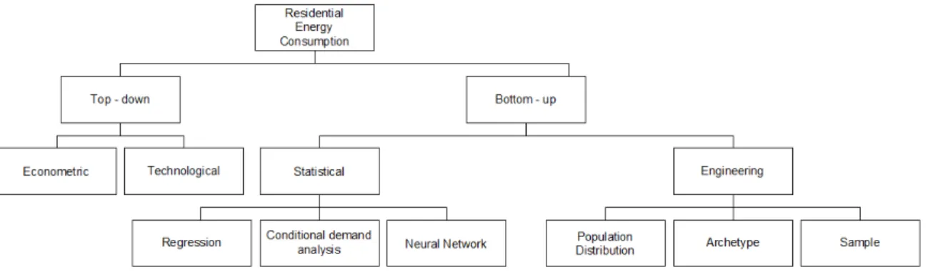
Heiple and Sailor [6] combined their work on geo-spatial modelling and on a prototypical building approach. This approach is applied to large U.S cities to obtain day-specific estimation and his model is also based on engineering sciences. Based on Swan and Ugursal [7] classification 1.2, Heiple and Sailor [6] couple the statistical and the engineering aspects, which attest that techniques can be coupled.

Swan and Ugursal [7] and Kavgic et al. [8] agree on the way of classification of residential energy consumption models, but in addition, Kavgic reviews the different bottom-up approaches to estimate the baseline energy demand of existing buildings stock. He shows that bottom-up building physics stock models are used to explicitly determine and quantify the impact of different combinations of technological measures on delivered energy use.

Popescu et al. [9] develops a simulation and prediction MATLAB model for the space heat-ing consumption of buildheat-ings connected to a partially-controlled system. Statistical and neural network modelling are used to develop the model and fix parameters as the wind velocity, the solar radiation or the human behaviour. Following the Swan’s classification1.2, Popescu’s model is listed in Bottom-up > Statistical > Neural network.

(18)

1.2 Building engineering physics 15

1.2 Building engineering physics

1.2.1 Energy consumption parameters

The aim of this part is to present parameters that impact the building energy consumptions. Main factors that affect energy consumption in buildings are clearly identify by scientists. Depending on the level of precision needed, some parameters are essential while other can be considered or not. According to Ratti et al. [10], climate is unmanageable but guides choices of construction which are made by urban planners, designers, architects and system engineers. Urban context, thermo-physical of the building envelop, systems efficiency and behaviour of occupants are con-sidered for several scientists like Ratti et al. [10] and Popescu et al. [9] as minimal and sufficient for simple calculation of the energy performances.

The impacts of the following parameters are not quantified but give an overview of the diversity of parameters:

• Climate:

– Temperature

– Latitude and longitude

– Wind velocity – Relative Humidity – Solar radiation • Occupants: – Number of occupants – Activity – Behaviour

– Opening and closing of windows

• Urban context:

– Close and distant obstructions

– Attachment to heated rooms

– Urban organization

• Buildings:

– Size and shape

– Heat transfer coefficients U – Wall and glazing surface

– Albedo

– Air renewal

– Orientation of glazing • Systems:

(19)

– Temperature setpoint – Devices power and efficiency

For each building these parameters can be quantified and are for most of them manageable. For historical, cultural and geographical reasons, urban contexts, buildings and systems parame-ter change. For instance, urbanism laws evolve with the time, prospect rules fix maximal heights of building depending on the width of streets and so close obstructions impacts are different depending on the laws.

Buildings can be classified by typology, for instance by climate (Chen et al. [11]), by shape (Zeferos et al. [12]) or by age as it is often the case (Caldera et al. [13] and Dorfner [14]). Classifications are not limited to one parameter, in the present project a classification by year of construction associated to a differentiation by size (collective or individual building) is made.

1.2.2 Energy performance

The energy performances directly depend on the quality of the building envelop which is the main parameter urban planners and architects can act on. Thermal regulations fix standards and features that changed with the time. Indeed, buildings built under the first thermal regulation of 1974 are less efficient than those built under the lasts regulations because targets in terms of bioclimatic needs1 _{and in term of energy consumptions change from one regulation to another.}

Softwares, as Perrenoud, accurately calculate the energy consumptions and all needs for individual buildings. But thermal studies are long and expensive because it is necessary to inform the software of the composing of walls, windows and all thermal bridges. These studies are based on numerical methods that simulate the maximum detailed components of buildings. That is why it is impossible to lead a campaign of EPCs at urban scales and why the statistical approach is selected.

To get an interesting building energy evaluation of a district the maximum parameters listed in the subsection 1.2.1 should be taken into account in the model. When the amount of input data is limited and in order to take into account urban context parameters and geometries, geo-localized approaches are adapted and powerful. Geographical Information Systems (GIS) work

on the Structure Query Language (subsection 1.4.2) and permit to complete the model with

informations that data bases do not give.

1.3 Data Bases

1.3.1 National institutes

Data are not centralized in one single institute, but in several data file depending on what they treat. It is important to notice that comparison between similar data can lead to significant differences due to the updates or due to the count method and references. Databases are often

1

Indicator used in the Thermal Regulation 2012 that evaluates the sustainable performances of the project, that is to say the envelop performances

(20)

1.3 Data Bases 17

private and they are either charged or given in case of partnership. Here is a non-exhaustive list of specialized institutes:

• IGN: French National Geographic Institute specialized on geodesy, geography and aerial photography. The institution products mainly topographic and road maps of France but also of some other countries.

• INSEE: French National Institute for Statistics and Economic Studies. It collects and publishes informations on the French economy and society, which is useful for Top-down modelling. This data-base is given from the national scale to the IRIS, which are French districts.

• Meteo France: French national meteorological service. It collects and stores meteorolog-ical data. Weather informations are unavoidable to model thermal situations to represent external excitation as the temperature, wind, rain, pressure or solar radiation.

• FILOCOM: French communal accommodation files. Households data built by the local taxation centre (DGI) on buildings features and occupation. The data are geo-referenced and so compatible with any GIS but are confidential.

• Extra data can be available from other institutes, as Perval which are managed by public notaries. We can also find energetic file as the CEREN which is a French statistical observatory energy demand or ENERDATA which makes researches on the global energy industry.

Databases are used by most organizations for their business operations and the interest of geo-referenced them makes them more powerful, this is the aim of Geographical Information Systems.

1.3.2 Maps databases

If data of national institutes are insufficient to feed a project, web mapping services applications can help to complete a database. Nowadays, web mapping services are varied and have different aims, the following list presents some of them and their uses:

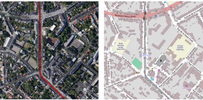
• Google Maps provides high-resolution aerial or satellite images for most urban areas all over the world. Not all areas on satellite images are covered in the same resolution. The powerfulness of Google Maps is to give an overview of buildings with high accuracy of their shape, disposal and morphology (Figure 1.1(left)).

• Google Street View is a technology featured included in Google Maps that provides panoramic views from positions along streets. It permits to the user to virtually walk in cities and visualize with high accuracy façades of buildings, morphologies, types, number of windows and so on.

• OpenStreetMap is a collaborative project also called Wikipedia of maps, where all In-ternet users browsing the web can contribute to the creation and digitization of maps. It

(21)

does not show images, but maps close to cadastral plans. They are useful to differentiate activities and feed databases (Figure 1.1(right)).

Figure 1.1: Comparison of satellite map of Google Maps (left) and collaborative map of Open-StreetMap (right) of the same part of Nantes shows different informations

To use data from national databases and additional informations collected from web mapping, Geographical Information Systems store, manipulate, analyse and manage all data under a table form that work with Structure Query Language (SQL) spatial language and which is called geo-database.

1.4 Geographical Information Systems (GIS)

1.4.1 History and functionality

GIS is an old tool used to link data and spatio-temporal location. In 1854, Doctor John Snow was the first scientist to draw a map to reveal phenomenon, as report Kari McLeod [15]. Snow held a study on the epidemic of cholera in the Soho district of London, by locating his patients and where they drew their water. Thanks to this geographical method, he demonstrated that a well was the source of contamination. This anecdote, is far from the subject of this report but illustrate the potential of this information system. Nowadays, GIS are used in several cases as for instance in environment, transportation, energy, defence, health, safety or research. Information systems are not only automatic mapping system, there are more decision supports.

Nowadays, lots of GIS are spread on the market; ArcGIS, Arcmap, Mapinfo, AutoCAD for the most renowned and they all have their specificities. OrbisGIS is a Geographical Information System, developed by the Institute on Urban Sciences and Techniques, dedicated to scientific

(22)

1.4 Geographical Information Systems (GIS) 19

modelling and simulation in urban context. This software done in Java is capable of displaying, manipulating and creating vector and raster spatial data [16]. Information systems stock rasters, vectors and alphanumeric data as thematic layers, they can be compared, combined or analysed in new relevant layers of a particular problematic with particular attributes.

According to Church [17] five components are essential to have functional GIS. In addition to data we presented on the previous section, an efficient software and computer are fundamental to avoid bugs and to have efficient compilations. Moreover, the operator should be a specialist and methods should be followed to succeed in any project.

1.4.2 Structure Query Language (SQL)

Databases are organized collection of data used to classify information and call attributes. To order these attributes, there is a special purpose programming language, SQL created in 1974, able to data insert, query, update, delete and data access control. This language permit to deal with tables more conveniently than Excel files.

In the field of buildings in a neighbourhood, databases have initially a minimum of two attributes; a number of identification and a valid geometry. Thanks to the SQL language other attributes can be get as perimeters and areas. Then, databases inform the GIS of others attributes as the height of buildings and so new other attributes can be computed as the volume for instance.

1.4.3 Projections

Projections are mathematical transformations that take spherical coordinates (latitude and lon-gitude) and transform them to a planar coordinate system able to make geometrical calculations

on SIG. According De Floriani et al. [18], in the handbook of computational geometry and

its chapter on applications of computational geometry to GIS, there are 3 main kinds of map projections, the cylindrical (Mercator projection), the conical (Lambert 93) and the azimuthal (Gnomonic projection). Coordinates from different projections cannot be compared without post-transformation.

1.4.4 Possibilities

Geographical Information Systems are used in a wide variety of applications as in history, hy-drology, transportation, crime, renewable energy and all activity sector that can be localized.

In the energy field several experiments with various objectives have been lead. In her work

Dorfner [14] used GIS to determine the annual energy demand for heating rooms on 200×200

m2 grids. The originality of her work is to integrate different heating technologies to the yearly energy demand in order to design a district heating. GIS were also used by Mavrogianni et al. [19] to evaluate the impact of urban built form and heat island effect on the levels of domestic energy

consumption. Heiple and Sailor [6] compare two approaches, top-down and bottom-up, and

combine annual building energy simulation for city specific prototypical buildings and available geospatial data in a GIS framework. Finally, hourly results can be extracted for any day and exported as a raster output at a spatial scale as fine as individual parcel.

(23)

Whatever is the project, Geographical Information Systems are used as automatic map sys-tems but are chiefly a tool able to generate results exploitable for decision support of project.

1.5 Approaches and models

1.5.1 Top-down and Bottom-up strategies

Top-down and bottom-up are families of strategies of information processing and knowledge ordering. They are adapted from districts to international scales and to several study domains. Each modelling technique relies on different levels of input information, different calculation or simulation techniques, and provides results with different applicability (Swan and Ugursal [7]). The following sections detail the top-down strategy and the bottom-up strategy. The Figure 1.2 summarize the classification of modelling approaches of the energy demand for the residential sector.

Figure 1.2: Hierarchical classification of approaches of residential energy consumption modelling. Source: Swan and Ugursal

• Top-down techniques are adapted to determine the impacts on the energy consumption after a change on a long time scale based on economics parameters. They treat the residential sectors as energy sinks and are used for supply analysis based on long-term projections of energy demand by accounting for historic response. This strategy implies simple data and models but is limited face to sudden changes. The Top-down technique often use a statistical approach to model the energy demand.

• Bottom-up techniques model detailed consumption for a small scale, based on engineering data, as the geometries, materials and all physical parameters impacting the system. By extrapolating the estimated energy consumption of this representative set of buildings to a bigger scale a global estimation can be done. The limits of this strategy is often the difficulties to get the input data and the complexity of systems, this often lead to long time calculations. However, slight changes and local phenomena can be easily modelled. As for the top-down technique, the bottom-up method generally follows a statistical approach but which can be developed in parallel to an engineering approach.

(24)

1.6 Modelling parameters 21

1.5.2 Variety of models

The Table1.1presents a review of thermal models based on the bottom-up approach. It details for each example of model: an equivalent example which follow the general method, the basics which explain how models work, the inputs and outputs of each model and then the advantages and limits.

Steady state

The calculation method 3CL-EPC [20] is based on the energy balance of buildings that is to say that for a given period of time the energy entering in the building plus the internal production minus the energy leaving is constant. Sankey diagrams are specific types of flow diagram, to visualize energy transfers, in which the width of arrows shows proportionally the flow quantity. To estimate the energy needs of buildings, the method is first to calculate heat losses through the envelop (walls, windows, doors, thermal bridges and air renewal), then to determine the inertia, the environmental solicitations and internal gains. The last fundamental parameter for a static approach is the heating degree hour which depend on the location and so the external temperatures during the heating season. An algorithm organizes these input parameters to give the annual heating needs of the studied zone.

Equivalent nodal network

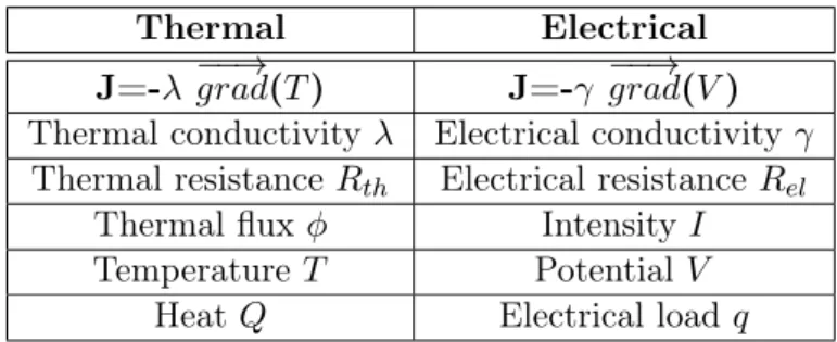
Davies [25] was a precursor and explained that electrical analogy draws a parallel between heat transfers and electrical currents. The thermal balance is equivalent to the electrical current conservation equation for each node. The Table1.2summarize the analogy between the electricity and the thermal.

In the equivalent node network method, the building is approximated to a set of nodes, that can be assimilated to homogeneous temperature zones or parts which have limited influence on the heat stored. The thermal coupling between nodes are represented by equivalent conduction where some nodes receive heat sources. The method can be considered as a method of finite differences, the whole building is divided into zones of elements of varying size. The development of an equivalent nodal network requires a good understanding of the physics building and clear objectives. Then the number and disposal of capacitors and resistors are determined in function of the building and objectives.

1.6 Modelling parameters

Databases help to feed the algorithm of useful data, but do not have parameters in link with geographical attributes. A preliminary step before the development of any algorithm is then to prepare input data that influence the study. The parameters presented in this part are the attachment, the orientation, the obstructions and some words explaining how to take into account the occupancy and appliances.

(25)

Categories of thermal mo dels a Example Basics Input Output A dv an tages Limits Steady State 3CL-EPC / F renc h Diag-nostic [ 20 ] Thermal mo del to esti-mate the energy consump-tion o v er a y ear Buildings char-acteristics (heat losses, inertia, a v er-age temp eratures, heating systems) Mon thly or an-n ual consumption (k W h/m 2 /y r ) Easy use Occupan ts not included No p o w er profile R C Cir-cuit Anal-ogy 5R2C / Kampf [ 21 ] Building mo del assimi-lated to an electrical cir-cuit (Resistances and Ca-pacities) Buildings char-acteristics (heat losses, inertia, hourly temp era-ture) P o w er profile Go o d accuracy P ossible div er-gence if time step to o long or inertia to lo w Simple Dynamic ESP-r /Stra-chan [ 22 ] Based on a finite v ol-ume approac h where it solv es a set of conserv ation equations. Also relev an t for other applications than energy Buildings charac-teristics (shap e, en vironmen t, installations, v en tilat io n ) Dynamic output Flexibilit y , Wide p ossibili-ties Long learning time, Need lots of data Resp onse F actor Hyiama [ 23 ] Calculation of a resp onse at a uni t excitation Studied parameter. P o w erful for single parameter study Corresp onding re-sp onse F ast calculation Easy use Not flexible Ap-pro ximated Numerical/ Finite Dif-ferences Cro wley [ 24 ] Represen tation b y equiv a-len t thermal net w orks, the solution is obtained b y solving a system of equa-tions represen ting the heat flo w b et w een the elemen ts Buildings charac-teristics (shap e, en vironmen t, installations, v en tilat io n ) 2D or 3D visualiza-tion High flexibilit y of the mo del Needs p o w erful computers Table 1.1 : Categories of thermal mo dels a The stea d y state and R C circuit a n alo gy thermal mo del are detailed in the c u rren t subsection

(26)

Thermal Electrical

J=-λ −−→grad(T ) J=-γ −−→grad(V )

Thermal conductivity λ Electrical conductivity γ Thermal resistance Rth Electrical resistance Rel

Thermal flux φ Intensity I

Temperature T Potential V

Heat Q Electrical load q

Table 1.2: Electrical/Thermal analogy

1.6.1 Attached walls

The wall attachment is a very important aspect of the modelling because it strongly influence the energy demand of a building. Indeed, attached buildings have external wall surface smaller than isolated ones, then the total heat losses are lower. Theodoridou et al. [26] in his work argues that the attachment to other buildings can even influence more than the age of buildings, which is justify as the older buildings feature does not have efficient thermal insulation.

Single zone building thermal models consider identical temperature for every building of the studied area. The heat conduction is by definition the transfer of heat energy of particles within a body due to a temperature gradient. In case of attached houses and based on Fourier’s law (Equation1.1), the heat flux between attached buildings is zero, because there is no temperature difference.

−

→_{ϕ = −λ ·}−−→_{grad(T )} _(1.1)

with: −

→_ϕ_{: Heat flux density [W.m}2_]

λ: Thermal conductivity [W.m−1.K−1] −−→

grad(T ): Temperature gradient [K.m−1_]

The shape ratio of a building is defined as the external surface divided by the gross volume. To reduce the energy consumption it is fundamental to get a low shape ratio and a heigh wall attached surface with surroundings buildings. According to Caldera et al. [13] the shape ratio is a significant parameter for calculating the heating needs per square meter and per year. With reliance, models consider that the percentage of surface of attachment is proportional to the heating energy saved, while considering only walls.

1.6.2 Orientation

The orientation is a parameter that can be only treated thanks to a GIS, never a data base give directly a value a orientation. Elsewhere, scientists debates to give a definition and to determine if the notion of orientation is meaningful for irregular building shapes. Most of researches, as

(27)

Duchêne et al. [27], fixed the orientation as the direction of the larger wall area, being based only on buildings footprints. Whereas, in their work, Andersson et al. [28] defined the orientation of the building as the direction in which the larger area of glass is facing. After the consideration of the orientation, researches determined the impact on the energy consumption. Andersson et al. studied the heating and the cooling load over a year for several U.S towns according to eight orientations (the four cardinal and four intermediate directions). Figure 1.3 shows the comparison of the orientation for the U.S city Nashville where the referenced orientation is the south and for a mixed climate in term of temperature. The paper presents how impacts the orientation on the energy consumption. For the modelled building of 100 m2_{, the setted disposal} of windows and other parameters, the orientation can lead to a maximum heat load difference of 1 MWh for the heating period, this difference correspond to 10 % of the final consumption.

To confirm Andersson’s work, Zerefos et al. [12] assure that the external shape of a building change significantly its energy consumption, regardless of the materials and the usage in terms of schedule, because the geometry change angles of incidence from solar radiation.

Figure 1.3: Relative variation of heating, cooling and total load according to the orientation of the building, in Nashville, Tennessee. Source: Andersson et al.

1.6.3 Obstructions

Obstructions are generally classified in two classes, the distant ones which are generally assimi-lated to the relief and the close shadows due to the direct surroundings environment as buildings or greeneries. For Nikoofard et al. [29] the orientation, size and distance of the neighbouring object determine the magnitude of the shading effect on the heating and cooling energy require-ment. Some buildings can be totally bereft of solar energy, which implies heating needs much more high than without obstruction. Moreover, due to the lower altitude of the sun and its shorter azimuth arc during the winter months, a neighbouring object located on the south side of a house was found to have a larger impact on the heating energy requirement than that of objects located on the other sides. Planting trees around a house can give the advantage of reducing cooling energy requirement in summer and eliminate the disadvantage of increasing heating energy requirement in the winter.

(28)

Full studies of the thermal irradiation are possible with softwares as Solène2_{. With this kind} of software, spatial and temporal parameters are taken into account for the simulation of the solar irradiation of each façade of each building. A betterment would be to develop an urban 3 dimensions SIG able to work under OrbisGIS but with the functionality of Solène.

A sub-aim of the project is to use OrbisGIS, the corresponding difficulty is to consider the time and so the sun-path. A possible method to simulate obstruction is to draw the shadows of the building, and observe is the surroundings buildings are impacted. GIS, is able to get results as shown in Figure 1.4where the shadow is drawn for a considered and fix time of the day.

Figure 1.4: Buildings shadow get from a Geographical Information System

1.6.4 Occupancy and appliances

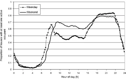
Richardson et al [30] modelled the domestic occupancy in order to estimate the energy consump-tion. Energy uses in homes is highly dependent on the activities of the residents. The timing of energy use, particularly electricity, is highly dependent on the timing of the occupants’ activities. Figure1.5, shows the proportion of houses with at least one active occupant over an experimental period of 50 days in an individual house. As expected, there is minimal activity during the night (00:00 to 07:00), some activity (at home) during the day and most activity during the evening. This example shows a tendency of the occupancy profile of a house but depends on numerous parameters often complex to model.

Activity Metabolic rates [M]

Reclining 46 W2/m 0.8 Met

Seated relaxed 58 W2/m 1.0 Met

Standing relaxed 70 W2/m 1.2 Met

Car driving 80 W2/m 1.4 Met

Domestic work 116 W2/m 2.0 Met

Washing dishes standing 145 W2/m 2.5 Met

Running at 15 km/h 550 W2/m 9.5 Met

Table 1.3: Metabolic rates according to human activities, Source: INNOVA

However, the study of the domestic occupancy also lead to information about the internal gain in order to heat the space. Indeed, bodies produce energy, called thermal metabolism, due

2

Solène is a software simulation of sunlight, illumination and heat radiation adapted for architectural and urban projects, developed by the CERMA laboratory

(29)

Figure 1.5: Aggregated individual active occupancy profiles for weekdays and weekend days. Source: Richardson

to the water and food oxidation, according to Denzer and Young [31]. The released energy is strongly function of the activity and its unit is the MET [M] (1 M = 58.15 W/m2_{). The total}

metabolic heat for a body depends on his activity and its morphology. Based on Table 1.3

(INNOVA [32]), the total heat for a reclining person would be 82.8 W and for someone having a medium activity at home would be 208.8 W. According to FILOCOM’ statistics [33], the average surface per person in households is 35.6 m2_{. Then knowing the occupancy profile it is easy to} estimate the heat gain per square meter for a dynamic simulation. In addition to heat gain due to the metabolism, buildings equipments, as electrical appliances and lightings, also participate in the heating of rooms. The thermal power released by electrical appliances is nearly proportional to its electric power. Morel and Gnansounou in the EPFL’s report [34] inform that to calculate precisely the energy gain due to appliances, a full study on devices is necessary in term of number and electrical power.

Finally, Morel and Gnansounou [34] conclude saying that the aggregation of the thermal power due to the metabolism and appliances leads to an average of 5 W/m2 _{in households.}

Conclusion

This state of the art permitted to present essential elements of the project, as databases, GIS, physics in buildings and energy demand models at local scales. Moreover, this bibliographic analyse presents a diversity of modelling approaches (physic, statistic, geographic, top-down, bottom-up ...) that can often be coupled between them. The objective of this Master thesis is to explore the bottom-up approach by integrating Geographical Information System to a statistical approach. The secondary objective is to get a flexible model, adaptable to different districts but also to different scales. However, the approach implies to have relevant data field (technical data of buildings for instance). To develop a new model and based on the existing works, input parameters should be operational to feed the algorithm, this is the main topic of the next chapter.

(30)

Chapter 2

Spatial analysis

This chapter presents the existing databases available at local scale, the prototypical approach selected and the preparation of input data using OrbisGIS queries. Limits and hypothesis of the model are presented all along the chapter. The simulation is done on Saint Félix, district of Nantes, and is associated to projects realized in Ecole des Mines de Nantes by Monteil [4] and Garcia [5] in order to compare approaches and results.

2.1 Data selection

2.1.1 Data base selection

The selection of the more appropriate database is fundamental for the following of the work. Indeed, it should contain the necessary attributes to be able to exploit it and to feed the algorithm. The available databases are:

• Topographic: Type of map characterized by large-scale detail and quantitative representa-tion of relief.

• Cadastral: Type of map which includes details of the ownership, the occupancy, an accurate location and the dimensions.

• Plot (Parcel): Type of map which represents parcel of land owned by owners with buildings, yards, plots and names of streets.

In addition to differences in geo-localized data due to projections explained in the subsec-tion 1.4.3, there are several differences between layers. For instance, topographic maps, got from Lambert II extended conic projection contains height attributes, but attached houses and buildings are considered as only one making this layer not exploitable for our project. Moreover, mismatches between two layers, as shown in Figure2.1, cancel the possibility to merge two tables because none data are common between the two. These problems lead to manual and automatic update on OrbisGIS.

(31)

Figure 2.1: Displaying of mismatch between plot map (in grey) and topographic map (in pink)

The final selection is given to the plot database as a base of the work, because it has initially differenced buildings, that is to say, that attached buildings are not gathered in only one but separated.

The choice to be focus only on undifferentiated (residential and heated locals) buildings is done, deleting industrial and remarkable infrastructures. This choice is assumed in order to make a simpler model and because the district is mainly residential. Indeed, a typological approach is valid for buildings of the same categories and materials use to build factories are not the same than to build houses.

2.1.2 Prototypical approach

The fundamental requirement for the development of a statistical model is the selection and the evaluation of the most influencing parameters. A sensibility analysis is a solution to create rep-resentative classes. The initial choice of the IRIS_0409, Saint-Félix, is justify by an equilibrated distribution of houses depending on the period of construction (Figure 2.2), a representative number of persons per household and an average surface of households. The objective of the typological approach is to gather buildings by classes.

The first discrimination variable choose is the age of construction because material, urbanism and architecture significantly change during the last century. The following list presents the prototypical division by age of construction and a brief explanation of dates done by Graulière [35] and APUR [36]:

• Class 1: Before 1915. Construction with local materials (stones, terracotta or earthen). Thick and heavy walls leading to buildings with high inertia. Low efficiency of the envelop. • Class 2: Between 1915 and 1948. Stones or bricks buildings make envelops buildings globally inefficient but generate limited thermal bridges due to a high compactness ratio. • Class 3: Between 1949 and 1974. Period of construction very inefficient due to a fast

construction post war. Thin walls, high glazing surface, untreated thermal bridges and so on.

(32)

2.1 Data selection 29

Figure 2.2: Repartition of number of buildings according to their age and their type for Saint-Félix. Source: Monteil

• Class 4: Between 1975 and 1989. Establishment of the first thermal regulation after the first oil shock. The insulation is systematic.

• Class 5: After 1990. Date of the second thermal regulation which result in buildings less energy consumer. Creation of other classes after 1990, for thermal regulation of 2000, 2005 and 2012, is not done due to limited number of buildings even if performances still become better.

The second variable of discrimination concern the size of buildings and is called "Type" in calculations we have 4 types detailed in the following list:

• Type 1-3: Collective buildings. Collective is defined as buildings with a number of floors higher than 2. Type 1 means that the building is attached to another one while type 3 means that it is isolated

• Type 2-4: Individual house. Individual is defined as houses with a number of floors equal or lower than 2. Type 2 means that the house is attached to another one while type 4 means that it is isolated.

In most applications types 1+3 and 2+4 are gathered because the Geographical Information System, OrbisGIS, automatically computes the attachment of buildings. However the differenti-ation is interesting to study the impact of the attachment to the energy consumption.

(33)

2.1.3 St Félix district specifications

The Figure2.3shows the geographical limits of the district St Félix, №441090409 of INSEE code [37], in the town of Nantes. It is located in the center/north part of the city beside the river Erdre and is inhabited by 3245 people distributed in 2015 households and 849 buildings. The neighbourhood is mainly residential and the two remarkable buildings kept for the simulation are the school (Groupe scolaire Felloneau) and the department store (Intermarché).

Figure 2.3: Location of Saint Félix in Nantes, Source: INSEE

The following work on OrbisGIS participate in the creation of the model of St Félix district. The plot database is a geographical layer which contains buildings footprints represented by polygons. Each polygon is associated to several data. First, a login is attributed to each geometry for manipulations. Secondly, the geometry of each polygon is stored to make the link between the maps and the database. The last information available and usable on the initial database is the kind of buildings (residential, remarkable and industrial). Queries on OrbisGIS and attributions of other data are detailed in the following section2.2, they permit to get input data to feed the algorithm and consequently energy consumptions.

2.2 OrbisGIS

2.2.1 Classification by type

As presented in the previous section, the choice of data source is the plot (parcel) database. However, it was necessary to make some update and corrections as erasing garages and cabins of the layer, because they are not heated. Moreover, some invalids geometries of the layer as shows Figure 2.4and2.5 are edited and corrected to get valid input data.

(34)

2.2 OrbisGIS 31

Figure 2.4: Geometrical modification of the building №695, the left part is before and right one is after the modification

Figure 2.5: Use of Google map to modify the geometry of the building №695

Thanks to the subsection 2.1.2 on the typological approach, the age is determined in ac-cordance with the work of Monteil [4], Figure 2.6 and Google Street View. Classes of age are determined based on the morphology of buildings. Renewal of buildings, like changing aeration systems, installing double glazing or isolating the envelope of the building are not considered and so, effective energy consumptions and theoretical ones can have significant differences. These changes modify considerably the consumption but are not detectable on Street View. Direct field study on the district permits to see real situation and to confirm or infirm what is on map data bases.

(35)

(36)

2.2 OrbisGIS 33

2.2.2 Number of floors

First, it is important to know the height of buildings because it permits to identify the repartition of individual houses and apartment buildings. If the number of floors is lower or equal than two, then the buildings are considered as individuals, therefore buildings of more than two floors are considered as apartment buildings. Secondly, knowing the number of floors, it is easy to estimate the height of buildings by making the hypothesis that the height per floor is 2.5 meters1_{. This} information is essential to calculate the air volume to heat.

The initial topographic database contained the gutter height of buildings but after verification they did not feet with the reality and then attributes were considered as wrong. Instead of estimating the real height of buildings, the number of floors were counted and feed in a new database.

2.2.3 Glazing Ratio (GR)

The GR is defined as the percentage of glazing on a building side. This ratio is used for calculation of solar gains and conduction heat losses. To calculate it, a statistical study has been led, for each period of construction (periods 1, 2, 3, 4 and 5) and both types of buildings an average of 10 measurements are done on random façades (except attached walls) thanks to Street View. The results of the study are summarized on the Table 2.1. Despite the fact that the determination of the GR actually does not use OrbisGIS a program based on orientation (south/north and street/yard) of façades and the age could be programmed for further applications.

This statistical study led us to the conclusion that depending on the age of building, the evolution of the GR and so of the architecture is significant. Indeed, between the first and the last class of age the proportion of glazing is doubled for the individual houses and quadrupled for blocks of flats.

GR (%) Individual houses Apartment buildings

Before 1915 16.4 11.2

1915-1948 16.2 13.4

1949-1974 26.0 28

1975-1989 25.4 45.2

After 1990 32.2 43.6

Table 2.1: Glazing Ratio (%) according to age and type of buildings

2.2.4 Attachment

The study of attached houses is essential for the calculation of the heating energy needed. In-deed, in detached houses the heat which goes through the envelope is lost and released outside. However, in situations of attached houses, the heat transfer goes through walls but is given to the besides houses and in the same time the heat from surrounding buildings is recovered.

1

(37)

The term attached perimeter on GIS informs on which side of buildings there is no heat losses through external walls. As illustrated on the Figure 2.7, there is the perimeter in black where the heat is not lost and in grey the perimeter where the heat is released in the atmosphere. In the developed model there is no distinction between external walls oriented to the dooryards and the ones oriented to the streets as APUR [36] did. Moreover, a limit of the actual model is that the height differences of buildings are not considered. Indeed, in the reality a 3 floors building attached with a 2 floors building, does not have the last floor which recover the energy from the second building, while in the model it does. This might be identify as an important limit but in Saint Félix there is very few discontinuity of building height, never an apartment building is attached to an individual house. The difficulty, on OrbisGIS is to discretize buildings to study only the one part of the perimeter or one façade.

Figure 2.7: Visualization of the two kinds of perimeters

As explained in the previous paragraph the measure of the attached perimeter is fundamental for the calculation of the heating needs. Here below is method and the SQL code developed to get the attached length as output:

• Step 1: Measure of the common length between two attached houses. One building can be associated to several lengths.

SQL: CREATE TABLE perimetremitoyen AS SELECT a.*, ST_Length(ST_Intersection

(a.the_geom, b.the_geom)) AS longueur FROM attributs a, attributs b WHERE (a.ID!=b.ID AND ST_Intersects(a.the_geom, b.the_geom));

• Step 2: We are interested in the length for each building so we gather results grouped by making the sum of the length. The result of this query is a table which contains the attached length of each attached building.

SQL: CREATE TABLE perimetermitoyen AS SELECT ST_UNION(the_geom) AS the_geom,

ID, Sum(longueur) AS perimetremit FROM perimetremitoyen GROUP BY ID;

• Step 3: The next step is to merge these values to the table of all others attributes.

SQL: CREATE TABLE jointure AS SELECT a.*, b.perimetremit FROM attributs a

LEFT JOIN perimetermitoyen b ON a.ID=b.ID;

• Step 4: Then we have to fix zero to detached houses that is to say buildings without attached length.

(38)

2.2 OrbisGIS 35

2.2.5 Orientation

As we saw during the literature survey, the general orientation of buildings is complex and the approach is debatable. First the orientation was define as the angle between the longest axis of the bounding rectangle of the building and the east-west axis, this method and the algorithm are explained in AppendixA.1. But this definition is not totally satisfactory because it does not take into account attachment and consequently glazings. The study of the orientation lead to coefficient that traduce the fact that façades ar not always oriented to the south and so does not benefit of the maximal radiation. The Table 2.2 lists the corresponding coefficients (C1) in function of the direction of one façade and not the orientation of the building according to [36].

Orientations Coefficients (C1) South 1 South-East / South-West 0.86 Est / West 0.55 North-East / North-West 0.3 North 0.2

Table 2.2: Orientation coefficients in function of the direction of one façade. Source: APUR However the aim is not to associate a coefficient to façades but to the whole building. Having no informations on the repartition of windows on façades we make the hypothesis that they are equally distributed on external walls (by type and age of building as shown in the Table 2.1). Whatever is the shape of an isolated building or house, the overall orientation coefficient is always equal to 0.58. And the only parameter which changes this coefficient, is the corresponding attachment, that is to say the number of attachment (AP) for each building. The computation of the number of AP with a SQL query is very similar to the one presented in the subsection on building shadowing effects2.2.6, since both queries count elements in a geometry. A link between overall orientation coefficient and number of attachment is done here below:

• AP=0: Calculated coefficients are comprised between 0.55 and 0.6 and finally fixed at C1=0.58.

• AP=1: Several situations are possible. If the attached wall is along the east or the west axis there is no impact on the final coefficient and the coefficient is equal to 0.58. For all the other cases only 4 coefficients are attributed. If the south orientation is cancelled by a surrounding building then the corresponding coefficient is 0.48. If it is north the corresponding coefficient is 0.68. In addition two other intermediate coefficients are in-cluded where the shared walls have angles around 45◦_{. The coefficient is equal to 0.53} for the south obstructions and 0.63 for the north obstructions. Currently this is a main limit because this has to be done manually, which is possible for a district but not for a city.

• AP=2: The study showed that buildings with two attachments have nearly always the attached wall at the opposite side. This means that the resulting coefficient is always close

(39)

to 0.58 because of the symmetry of the situation.

• AP=3 and more: No laws are found for these situations which represent 3.5 % of the buildings of the district. Therefore, coefficients are calculated individually and the Figure 2.8presents an example of calculation:

Figure 2.8: Example of calculation of the orientation coefficient for an attachment proportion equal to 3

C1 = 3 × 0.3 + 5 × 0.3 + 3.5 × 0.86 + 1 × 0.86 + 1.5 × 0.86

3 + 5 + 3.5 + 1 + 1.5 = 0.54 (2.1)

The convenience of this method is debatable since some attributes2 _{should be feed manually,} but the resulting orientation coefficients and the further solar gains associated are well-estimated. A possible update of this limit would be possible if and only if buildings façades are studied individually.

2.2.6 Greenery and building obstructions

Shading by neighbouring buildings and trees impacts the energy requirement of a building by reducing the amount of radiant energy absorbed and stored by its thermal mass. In this model, only close overshadowing are taken into account, distant overshadowing, due to mountains for instance are neglected. Clouds and aerosols are already taken into account in the solar gain of the external solicitation. The aim of this section is then to take into account the micro climate of the district, which significantly impact the building energy consumption.

Greenery shadowing effects

The consideration of greenery around buildings leads towards a model based on buffers3 _{of the} vegetation layer. The model is static and the sun path is not include. In the developed model, the

2

For the case of St Félix, 29 % of buildings have an attachment proportion of 1 and 3.5 % have an AP equal or higher than 3.

3

Buffers in GIS are useful for proximity analysis, they create an area defined by a bounding region determined by a set of points at a specified maximum distance around a geometry

(40)

2.2 OrbisGIS 37

impact of the greenery shadowing is a coefficient which impact the solar gain when the considered buildings are included in the buffer of the layer vegetation. The Figure 2.9 shows the different kind of buildings, those which are impacted by the greenery (in red) and those which are not impacted (in blue). The chosen corresponding coefficient decreasing the solar gains is fixed at 10 % for the simulation but can be easily modify. To develop a more complete model a field survey could be lead to determine more parameters like the trees size or the kind of vegetation.

Figure 2.9: Impact of greenery on sun obstructions. The dark green is the vegetation, the light green is the buffer of 5 meters of the vegetation, red buildings are those into the buffer and the blue buildings are those which are not impacted by the greenery

Building shadowing effects

External obstruction influences the daylighting performance and the building energy consump-tion. The effect depends on the height of neighbouring buildings and the separations. When buildings are located close to each other, blockage of solar gain can be severe, particularly for the units on lower floors. The final effect on buildings overshadowed is difficult to estimate but

(41)

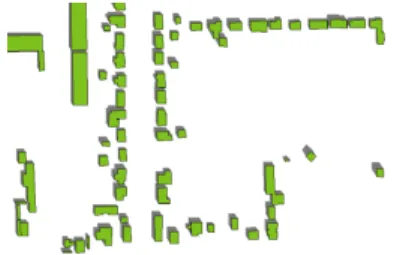
the impact seems to be limited since we consider only winter days in an region of low sunshine as Nantes area. The query is developed on OrbisGIS and here again based on the buffers. The method is to create buffers of size proportional to buildings high to represent the shadow of each ones that is to say when the declination of the sun is at 45 ◦_{. Then the number of buildings} which impact the studied one is considered as significant to estimate the obstruction. Based on the work of APUR [36] and once the number of obstructions determined, the association to co-efficients (Table2.3) is necessary to feed the algorithm. The following list presents the necessary steps on OrbisGIS to link the building environment to building shadowing coefficients:

• Step 1: Creation of a table with the geometry of buffers of each building, where the size of the buffer is equal to the high of the building. The result of this step is exposed in figure 2.10.

SQL: CREATE TABLE bufferbati AS SELECT ST_Buffer(the_geom, 3*3*etages) AS

the_geom, ID FROM attributs;

• Step 2: Link of the two tables where only couples which intersect themselves are kept.

SQL: CREATE TABLE join_intersect AS SELECT a.the_geom, a.ID, b.ID as ID_buff

FROM attributs a, bufferbati b WHERE ST_INTERSECTS(b.the_geom, a.the_geom);

• Step 3: Count of buildings in the buffer zone, by pulling the studied building (minus 1).

SQL: CREATE TABLE final AS SELECT ST_UNION(the_geom) AS the_geom, ID,

(count(ID_buff)-1) AS nb_bat FROM join_intersect GROUP BY ID;

• Step 4: Deleting of attached buildings.

SQL:

– CREATE TABLE buildingobstruction AS SELECT final.*, attributs.NB_MITOYEN

FROM final, attributs WHERE final.ID=attributs.ID;

– ALTER TABLE buildingobstruction ADD COLUMN nb_obstruction DOUBLE;

– UPDATE buildingobstruction SET nb_obstruction=nb_bat-NB_MITOYEN;

Number of obstructions 0 1 2 3 4 5

Associated coefficient 1 0.9 0.8 0.7 0.65 0.6

Table 2.3: Associated obstruction coefficient to the number of building obstruction As said, this method is improvable especially by taking into account the relative disposal of buildings. Indeed, a building can’t obstruct another building situated to the south.