VIRTIS-M-IR nadir and limb observations: variability of the O2(a1∆) nightglow spots

VIRTIS-M-IR nadir and limb observations:

variability of the O

₂

(a

1

∆∆∆∆

) nightglow spots

L. Soret (1), J.-C. Gérard (1), G. Piccioni (2) and P. Drossart (3)

(1) LPAP, Université de Liège, Belgium, (2) IAPS-INAF, Rome, Italy, (3) Observatoire de Paris-Meudon, France (Lauriane.Soret@ulg.ac.be / Fax: +32 4 366 9711)

Abstract

Individual nadir and limb VIRTIS-M-IR at 1.27 µm show that the O2(a1∆) nightglow emission is highly

variable. This variability is observed spatially, but also in term of intensity and altitude of the emitting layer over time. Apparent wind velocities have been deduced from the nadir observations, as well as the e-folding times. Limb observations show that an increase of the emitting layer altitude is observed near the cold collar region.

1. Introduction

The dynamics of the Venus atmosphere in the transition region between that governed by the retrograde superrotational zonal (RSZ) circulation (below 65 km) and that dominated by the subsolar to antisolar (SS-AS) circulation (above 130 km) is still not fully understood. The O2(a

1

∆) nightglow emission at 1.27 µm, whose emitting layer is located at ~96 km, can be used as a tracer of the dynamics in this transition region. A large amount of both nadir and limb observations have been acquired since April 2006 at this wavelength by the imaging spectrometer VIRTIS-M-IR on board Venus Express.

Nadir observations corrected from geometrical effects and thermal emission have been averaged in several previous studies [1, 5, 6] to generate a statistical map of the O2(a1∆) nightglow emission

(Figure 1). Such maps show that the emission peak is statistically located around the antisolar point. Intensity profiles have been extracted from limb images and deconvolved. Previous studies showed that the emitting layer is located at ~96 km [2, 5, 6]. This study now focuses on analyzing individual nadir and limb observations. Section 2 presents the variability of the oxygen nightglow in nadir individual data, from which apparent wind velocities and e-folding times have also been estimated. Section 3 shows latitudinal cuts of the Venus atmosphere

obtained with VIRTIS-M-IR limb observations and the emitting layer altitude variations.

Figure 1: Statistical map of the O2(a1∆) nightglow

generated with nadir VIRTIS-M-IR observations. [7]

2. Nadir observations

2.1 Variability of the nightglow spots

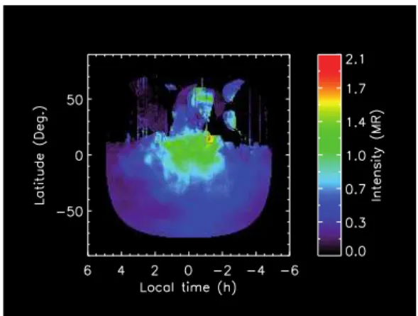
Figure 2 shows three examples of VIRTIS-M-IR nadir observations at 1.27 µm. Those examples already illustrate that the emission spot is not always located at the antisolar point and that the brightness of the emission can vary.

Such nadir observations have been processed with a blob-coloring technique in order to automatically extract the brightest patch from the image. The coordinates (latitude and local time) of the patch barycenter have been estimated and associated to the averaged intensity of the patch. Bright emission patches have been observed in almost any region of the Venus nightside covered by nadir observations (Southern hemisphere, from 19:00 to 05:00 LT), but the brightest ones statistically occur in the vicinity of the antisolar point.

EPSC Abstracts

Vol. 9, EPSC2014-36, 2014

European Planetary Science Congress 2014 c

Figure 2: Examples of individual nadir observations of the O2(a1∆) airglow structure. [7]

0 3 .0 1 .0 0 .5 2 .0 2 .5 1 .5 M R

Figure 3: Position and intensity of the nightglow spots on the Venus nightside. [7]

2.2 Apparent wind estimation

Nadir observations of a given sequence can also be grouped in order to generate series of consecutive images pointing at the same Venus nightside region in a limited period of time [4]. A total of 47 time series have been generated, allowing to follow the evolution of bright emission patches. The apparent wind velocities estimated through this motion tracking are shown in Figure 4: the displacements appear to be highly random both in magnitude and direction.

Figure 4: Map of the apparent wind vectors measured on the Venus nightside (dashed area). [7]

2.3 E-folding times

The variations of the bright patch intensity of each series of nadir observations have also been followed over time. Both intensity increases and decays have been observed during the time series. The e-folding times have been estimated. Decay times range from 72 to 2715 minutes, with a mean value of ~750 minutes. The mean rise time is ~1550 minutes. Increasing phases can be explained by a local additional supply of oxygen atoms from the dayside. The long decay time (exceeding the 75 min O2(a1∆)

radiative lifetime) can be interpreted as a combination of the radiative decay of the O2(a1∆)

metastable state and the lifetime of the O atoms.

3. Limb observations

Deconvolved limb profiles of a given sequence have been grouped together in order to generate global latitudinal cuts of the Venus atmosphere [3]. Some latitudinal cuts are shown in Figure 5. As observed in the nadir viewing geometry, multiple bright spots frequently occur simultaneously at several locations with different spatial extension, brightness and altitude distribution. An increase of the emitting layer is generally observed between 50° and 60° N. Also, the brightening in the high intensity regions often vanishes almost entirely within one day. These features suggest that either the transport from the day to the night side is more complex and time dependent than the global SS-AS circulation or that the efficiency of the turbulent downward transport on the nightside in the mesosphere-thermosphere transition region is variable.

Figure 5: Latitudinal cuts of the O2(a1∆) emission

over time. [3]

5. Summary and Conclusions

The subsolar to antisolar general circulation controls the statistical behavior of the O2 infrared nightglow

on time scales of months and years. On shorter time scales, the behavior of the emission spots is much more variable; spatially but also in brightness and altitude (especially near the cold collar region). Apparent displacement have been estimated but might not always represent an actual wind speed since the bright patches followed in this study sometimes change both in intensity and shape. In these cases, i) oxygen atoms within a given patch may not subject to a uniform motion or ii) it is also possible that the O2(a

1

∆) intensity variations results from a combination of changes in the downward fluxes of oxygen atoms or atmospheric density, or iii) the presence of gravity waves modifying the strength of the local vertical transport.

Radiative processes alone cannot explain the observed intensity decay observed in the Venus atmosphere but this apparent inconsistency can however be solved when considering the chemical lifetime of the atomic oxygen atoms which continuously produce O2(a1∆) molecules together

with the vertical transport time scales.

Still, the sources of these local enhancements (gravity waves, downwelling, enhanced eddy mixing) are still largely unknown.

Acknowledgements

We gratefully thank all members of the ESA Venus Express project and of the VIRTIS scientific and technical teams. This research was supported by the PRODEX program managed by the European Space Agency with the help of the Belgian Federal Space Science Policy Office. This work was also funded by Agenzia Spaziale Italiana and the Centre National d’Etudes Spatiales.

References

[1] Gérard, J.-C., Saglam, A., Piccioni, G., Drossart, P., Cox, C., Erard, S., Hueso, R., and Sanchez-Lavega, A.: Distribution of the O2 infrared nightglow observed with

VIRTIS on board Venus Express, Geophys. Res. Lett., 35, 2008.

[2] Gérard, J.-C., Soret, L., Saglam, A., Piccioni, G., and Drossart, P.: The distributions of the OH Meinel and O2(a1∆-X3Σ) nightglow emissions in the Venus mesosphere

based on VIRTIS observations, Adv. Space Res. 45, 1268-1275, 2010.

[3] Gérard, J.-C., Soret, L., Piccioni, G., and Drossart, P.: Latitudinal structure of the Venus O2 infrared airglow: A

signature of small-scale dynamical processes in the upper atmosphere, Icarus, 2014.

[4] Hueso, R., Sánchez-Lavega, A., Piccioni, G., Drossart, P., Gérard, J.-C., Khatuntsev, I., Zasova, L., and Migliorini, A.: Morphology and dynamics of Venus oxygen airglow from Venus Express/Visible and Infrared Thermal Imaging Spectrometer observations, J. Geophys. Res.,113, E00B02, 2008.

[5] Piccioni, G., Zasova, L., Migliorini, A., Drossart, P., Shakun, A., Munoz, A.G., Mills, F.P., and Cardesin-Moinelo, A.: Near-IR oxygen nightglow observed by VIRTIS in the Venus upper atmosphere, J. Geophys. Res., 114, 2009.

[6] Soret, L., Gérard, J.-C., Montmessin, F., Piccioni, G., Drossart, P., and Bertaux, J.-L.: Atomic oxygen on the Venus nightside: Global distribution deduced from airglow mapping, Icarus, 217, 849-855, 2012.

[7] Soret, L., Gérard, J.-C., Piccioni, G., and Drossart, P.: Time variations of O2(a1∆) nightglow spots on the Venus