Reduced Bond Graph via machine learning for nonlinear multiphysics dynamic systems
Texte intégral
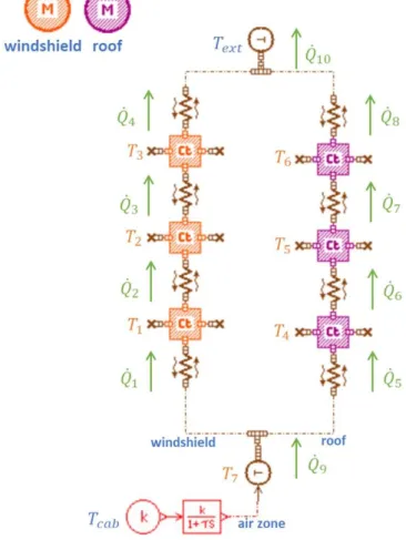
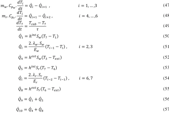
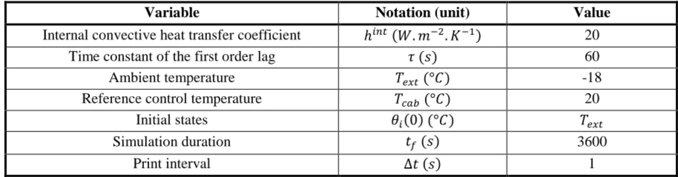
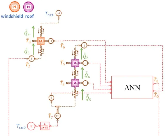
Figure
Documents relatifs
Background and Objectives: This paper presents the results of a Machine- Learning based Model Order Reduction (MOR) method applied to a complex 3D Finite Element (FE)
Among machine learning techniques for spoken dialogue strategy optimization, reinforcement learning [2] us- ing Markov Decision Processes (MDPs) [1, 3, 4, 5, 6, 7] and
• VISUALIZE (generally in 2D) the distribution of data with a topology-preserving “projection” (2 points close in input space should be projected on close cells on the SOM).
The fundamental mathematical tools needed to understand machine learning include linear algebra, analytic geometry, matrix decompositions, vector calculus, optimization,
Furthermore, we test our techniques on a number of real-world RDF machine learning classification datasets and show that simplification can, for the right parameters,
5.3 The complete n × n nonlinear system The common feature of the proposed neural network solvers presented in the previous sections, is their structure, characterized by the
“Echo State Queueing Networks: a combination of Reservoir Computing and Random Neural Networks”, S. Rubino, in Probability in the Engineering and Informational
For the training dataset an initial time limit of 4 seconds was used, doubled incrementally if all orderings timed out, until CAD completed for at least one ordering (a target
