HAL Id: hal-01671982
https://hal.inria.fr/hal-01671982
Preprint submitted on 22 Dec 2017
HAL is a multi-disciplinary open access
archive for the deposit and dissemination of
sci-entific research documents, whether they are
pub-lished or not. The documents may come from
teaching and research institutions in France or
abroad, or from public or private research centers.
L’archive ouverte pluridisciplinaire HAL, est
destinée au dépôt et à la diffusion de documents
scientifiques de niveau recherche, publiés ou non,
émanant des établissements d’enseignement et de
recherche français ou étrangers, des laboratoires
publics ou privés.
minimization. Application to computational biology
Cyprien Gilet, Marie Deprez, Jean-Baptiste Caillau, Michel Barlaud
To cite this version:
Cyprien Gilet, Marie Deprez, Jean-Baptiste Caillau, Michel Barlaud. Clustering with feature selection
using alternating minimization. Application to computational biology. 2017. �hal-01671982�
Clustering with feature selection using
alternating minimization.
Application to computational biology
Cyprien Gilet, Marie Deprez, Jean-Baptiste Caillau and Michel Barlaud, Fellow, IEEE
Abstract—This paper deals with unsupervised clustering with
feature selection. The problem is to estimate both labels and a sparse projection matrix of weights. To address this combina-torial non-convex problem maintaining a strict control on the sparsity of the matrix of weights, we propose an alternating minimization of the Frobenius norm criterion. We provide a new efficient algorithm named K-sparse which alternates k-means with projection-gradient minimization. The projection-gradient step is a method of splitting type, with exact projection on the
ℓ1 ball to promote sparsity. The convergence of the gradient-projection step is addressed, and a preliminary analysis of the alternating minimization is made. The Frobenius norm criterion converges as the number of iterates in Algorithm K-sparse goes to infinity. Experiments on Single Cell RNA sequencing datasets show that our method significantly improves the results of
PCA k-means, spectral clustering, SIMLR, and Sparcl
methods. The complexity of K-sparse is linear in the number of samples (cells), so that the method scales up to large datasets. Finally, we extend K-sparse to supervised classification.
I. INTRODUCTION
This paper deals with unsupervised clustering with feature selection in high dimensional space. As an application, we choose single-cell RNA-seq which is a new technology able to measure the expression of thousands of genes (20,000 genes) in single cells. Characterization of diverse cell types and their distinguishing features require robust and accurate clustering methods. However, clustering in high dimension suffers from the curse of dimensionality: as dimensions increase, vectors become indiscernible and the predictive power of the afore-mentioned methods is drastically reduced [1], [36]. In order to overcome this issue, a popular approach for high-dimensional data is to perform Principal Component Analysis (PCA) prior to clustering. This approach is however difficult to justify in general [45]. An alternative approach proposed in [18], [19] is to combine clustering and dimension reduction by means of Linear Discriminant Analysis (LDA). The heuristic used in [19] is based on alternating minimization, which consists in iteratively computing a projection subspace by LDA, using the labels y at the current iteration and then running k-means on the projection of the data onto the subspace. Departing from this work, the authors of [5] propose a convex relaxation M. Barlaud and C. Gilet are with I3S, Univ. Côte d’Azur & CNRS, F-06900 Sophia Antipolis. E-mail: [email protected], [email protected].
J.-B. Caillau is with LJAD, Univ. Côte d’Azur & CNRS/Inria, F-06108 Nice. E-mail: [email protected]
M. Deprez is with IPMC, Univ. Côte d’Azur & CNRS, F-06560 Sophia Antipolis. E-mail: [email protected]
in terms of a suitable semi-definite program (SDP). Another efficient approach is spectral clustering where the main tools are graph Laplacian matrices [33], [43]. However, methods such as PCA, LDA or, more recently SIMLR, do not provide sparsity. A popular approach for selecting sparse features in supervised classification or regression is the Least Absolute
Shrinkage and Selection Operator (LASSO) formulation [39].
The LASSO formulation uses the ℓ1 norm instead of ℓ0 [11],
[12], [20], [21] as an added penalty term. A hyperparameter, which unfortunaltely does not have any simple interpretation, is then used to tune the sparsity. The authors of [46] use a lasso-type penalty to select the features and propose a sparse k-means method. A main issue is that optimizing the values of the Lagrangian parameter λ [24], [46] is computationally expensive [30]. All these methods [5], [18], [19], [46] require a k-means heuristic to retrieve the labels. The alternating scheme we propose combines such a k-means step with dimension reduction and feature selection using an ℓ1sparsity constraint.
II. CONSTRAINED UNSUPERVISED CLASSIFICATION
A. General Framework
Let X(̸= 0) be the m × d matrix made of m line samples
x1, . . . , xm belonging to the d-dimensional space of features.
Let Y ∈ {0, 1}m×k be the label matrix where k ⩾ 2 is the number of clusters. Each line of Y has exactly one nonzero element equal to one, yij = 1 indicating that the sample xi
belongs to the j-th cluster. Let W ∈ Rd× ¯d be the projection matrix, ¯d≪ d, and let µ be the k × ¯d matrix of centroids in
the projected space XW :
µ(j, :) := ∑m1 i=1yij
∑
i s.t. yij=1
(XW )(i, :).
The j-th centroid is the model for all samples xi belonging
to the j-th cluster (yij = 1). The clustering criterion can be
cast as the within-cluster sum of squares (WCSS, [37], [46]) in the projected space
1
2∥Y µ − XW ∥
2
F → min (1)
where ∥.∥F is the Frobenius norm induced by the Euclidean
structure on m× ¯d matrices,
(A|B)F := tr(ATB) = tr(ABT), ∥A∥F :=
√
(A|A)F.
The matrix of labels is constrained according to
k ∑ j=1 yij = 1, i = 1, . . . , m, (3) m ∑ i=1 yij⩾ 1, j = 1, . . . , k. (4)
Note that (3) implies that each sample belongs to exactly one cluster while (4) ensures that each cluster is not empty (no fusion of clusters). This prevents trivial solutions consisting in k− 1 empty clusters and W = 0. In contrast with the Lagrangian LASSO formulation, we want to have a direct control on the value of the ℓ1 bound, so we constrain W
according to
∥W ∥1⩽ η (η > 0), (5)
where∥.∥1 is the ℓ1 norm of the vectorized d× ¯d matrix of
weights: ∥W ∥1:=∥W (:)∥1= d ∑ i=1 ¯ d ∑ j=1 |wij|.
The problem is to estimate labels Y together with the sparse projection matrix W . As Y and W are bounded, the set of constraints is compact and existence holds.
Proposition 1 The minimization of the norm (1), jointly in Y
and W under the constraints (2)-(5), has a solution.
To attack this difficult nonconvex problem, we propose an alternating (or Gauss-Seidel) scheme as in [18], [19], [46]. Another option would be to design a global convex relaxation to address the joint minimization in Y and W ; see, e.g., [5], [23]. The first convex subproblem finds the best projection from dimension d to dimension ¯d for a given clustering.
Problem 1 For a fixed clustering Y (and a given η > 0), 1
2∥Y µ − XW ∥
2
F → min
under the constraint (5) on W .
Given the matrix of weights W , the second subproblem is the standard k-means on the projected data.
Problem 2 For a fixed projection matrix W , 1
2∥Y µ − XW ∥
2
F → min
under the constraints (2)-(4) on Y .
B. Exact gradient-projection splitting method
To solve Problem 1, we use a gradient-projection method. It belongs to the class of splitting methods [14], [15], [29], [32], [38] and is designed to solve minimization problems of the form
φ(W )→ min, W ∈ C, (6)
using separately the convexity properties of the function φ on one hand, and of the convex set C on the other. We use the
following forward-backward scheme to generate a sequence of iterates:
Vn := Wn+ γn∇φ(Wn), (7)
Wn+1 := PC(Vn) + εn, (8)
where PCdenotes the projection on the convex set C (a subset
of some Euclidean space). Under standard assumptions on the sequence of gradient steps (γn)n, and on the sequence
of projection errors (εn)n, convergence holds (see, e.g., [6]).
Theorem 1 Assume that (6) has a solution. Assume that φ
is convex, differentiable, and that ∇φ is β-Lipschitz, β > 0. Assume finally that C is convex and that
∑
n
|εn| < ∞, inf
n γn > 0, supn γn< 2/β.
Then the sequence of iterates of the forward-backward scheme (7-8) converges, whatever the initialization. If moreover
(εn)n = 0 (exact projections), there exists a rank N and a
positive constant K such that for n⩾ N φ(Wn)− inf
C φ⩽ K/n. (9)
In our case,∇φ is Lipschitz since it is affine,
∇φ(W ) = XT(XW − Y µ),
(10) and we recall the estimation of its best Lipschitz constant. Lemma 1 Let A be a d× d real matrix, acting linearly on
the set of d× k real matrices by left multiplication, W 7→ AW . Then, its norm as a linear operator on this set endowed with the Frobenius norm is equal to its largest singular value, σmax(A).
Proof. The Frobenius norm is equal to the ℓ2 norm of the vectorized matrix, ∥W ∥F =∥ W1 .. . Wh ∥2, ∥AW ∥F =∥ AW1 .. . AWh ∥2, (11) where W1, . . . , Whdenote the h column vectors of the d× h
matrix W . Accordingly, the operator norm is equal to the largest singular value of the kd× kd block-diagonal matrix whose diagonal is made of k matrix A blocks. Such a matrix readily has the same largest singular value as A. □ As a byproduct of Theorem 1, we get
Corollary 1 For any fixed step γ ∈ (0, 2/σmax2 (X)), the
forward-backward scheme applied to the Problem 1 with an exact projection on ℓ1 balls converges with a linear rate towards a solution, and the estimate (9) holds.
Proof. The ℓ1 ball being compact, existence holds. So does convergence, provided the condition of the step lengths is fulfilled. Now, according to the previous lemma, the best Lipschitz constant of the gradient of φ
Algorithm 1 Exact gradient-projection algorithm Input: X, Y, µ, W0, N, γ, η W ← W0 for n = 0, . . . , N do V ← W − γXT(XW− Y µ) W ← Pη1(V ) end for Output: W
is σmax(XTX) = σ2max(X), hence the result. □
Exact projection. In Algorithm 1, we denote by P1
η(W ) the
(reshaped as a d × ¯d matrix) projection of the vectorized
matrix W (:). An important asset of the method is that it takes advantage of the availability of efficient methods [16], [22] to compute the ℓ1 projection. For η > 0, denote B1(0, η) the
closed ℓ1 ball of radius η in the space Rd ¯d centered at the
origin, and ∆η the simplex {w ∈ Rd ¯d | w1+· · · + wd ¯d =
1, w1⩾ 0, . . . , wd ¯d ⩾ 0}. Let w ∈ Rd ¯d, and let v denote the
projection on ∆η of (|w1|, . . . , |wd ¯d|). It is well known that
the projection of w on B1(0, η) is
(ε1(v1), . . . , εkd(vd ¯d)), εj := sign(wj), j = 1, . . . , d ¯d,
(12) and the fast method described in [16] is used to compute v with complexity O(d× ¯d).
Fista implementation. A constant step of suitable size γ is used in accordance with Corollary 1. In our setting, a useful normalization of the design matrix X is obtained replacing X by X/σmax(X). This sets the Lipschitz constant in Theorem 1
to one. The O(1/n) convergence rate of the algorithm can be speeded up to O(1/n2) using a FISTA step [7]. In practice we use a modified version [13] which ensures convergence of the iterates, see Algorithm 2. Note that for any fixed step γ∈ (0, 1/σmax2 (X)), the FISTA algorithm applied to Problem 1
with an exact projection on ℓ1balls converges with a quadratic rate towards a solution, and the estimate (9) holds.
Algorithm 2Exact gradient-projection algorithm with FISTA Input: X, Y, µ, W0, N, γ, η W ← W0 t← 1 for n = 0, . . . , N do V ← W − γXT(XW− Y µ) Wnew ← Pη1(V ) tnew← (n + 5)/4 λ← 1 + (t − 1)/tnew W ← (1 − λ)W + λWnew t← tnew end for Output: W C. Clustering algorithm
The resulting alternating minimization is described by Algorithm 3. (One can readily replace the gradient-projection
step by the FISTA version described in Algorithm 2.) Labels
Y are for instance initialized by spectral clustering on X,
while the k-means computation relies on standard methods such as k-means++ [2].
Algorithm 3 Alternating minimization clustering. Input: X, Y0, µ0, W0, L, N, k, γ, η Y ← Y0 µ← µ0 W ← W0 for l = 0, . . . , L do for n = 0, . . . , N do V ← W − γXT(XW − Y µ) W ← P1 η(V ) end for Y ← kmeans(XW, k) µ← centroids(Y, XW ) end for Output: Y, W
Convergence of the algorithm. Similarly to the approaches advocated in [5], [18], [19], [46], our method involves non-convex k-means optimization for which convergence towards local minimizers only can be proved [9], [37]. In practice, we use k-means++ with several replicates to improve each clustering step. We assume that the initial guess for labels Y and matrix of weights W is such that the associated k centroids are all different. We note for further research that there have been recent attempts to convexify k-means (see, e.g., [10], [17], [31], [35]). As each step of the alternating minimization scheme decreases the norm in (1), which is nonnegative, the following readily holds.
Proposition 2 The Frobenius norm∥Y µ − XW ∥F converges
as the number of iterates L in Algorithm 3 goes to infinity.
This property is illustrated in the next section on biological data. Further analysis of the convergence may build on recent results on proximal regularizations of the Gauss-Seidel alternating scheme for non convex problems [3], [8].
Gene selection. The issue of feature selection thanks to the sparsity inducing ℓ1 constraint (5) is also addressed in this
specific context. The projection P1
η(W ) aims to sparsify the
W matrix so that the gene j will be selected if∥W (j, :)∥ > 0.
For a given constraint η, the practical stopping criterion of the alternating minimization algorithm involves the evolution of the number of the selected genes (see Fig. 4 in Section III). In the higher level loop on the bound η itself, the evolution of criterion such as accuracy versus η is analyzed. We also note that the extension to multi-label is obvious, as it suffices to allow several ones on each line of the matrix Y by relaxing constraint (3).
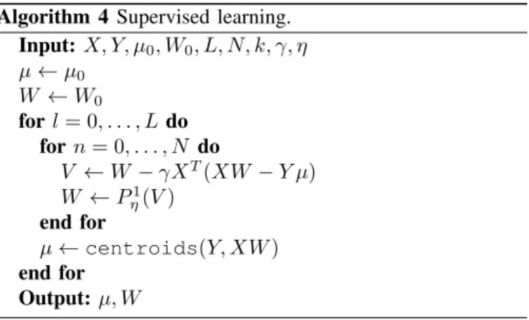
D. Supervised learning
As a final remark, we note that a straightforward modification of Algorithm 3 allows to address supervised classification. If
the labels Y are available, the simpler goal is to compute the matrix of weights W as well as the resulting centroids in the projected space. For the sake of completeness we include below the corresponding update of the algorithm 3. Experimentations in the supervised case are out of the scope of this paper and will be reported somewhere else.
Algorithm 4 Supervised learning. Input: X, Y, µ0, W0, L, N, k, γ, η µ← µ0 W ← W0 for l = 0, . . . , L do for n = 0, . . . , N do V ← W − γXT(XW− Y µ) W ← P1 η(V ) end for µ← centroids(Y, XW ) end for Output: µ, W
III. APPLICATION TO SINGLE CELLRNA-SEQ CLUSTERING
A. Experimental settings
We normalize the features and use the FISTA implementation with constant step γ = 1 in accordance with Corollary 1. The problem of estimating the number of clusters is out of the scope of this paper, and we refer to the popular Gap method [40]. We compare the labels obtained from our clustering with the true labels to compute the clustering accuracy. We also report the popular Adjusted Rank Index (ARI) [28] and
Normalized Mutual Information (NMI) criteria. Processing
times are obtained on a 2.5 GHz Macbook Pro with an i7 processor. We give tsne results for visual evaluation [42] for five different methods: PCA k-means, spectral clustering [43], SIMLR[44], Sparcl (we have used theR software provided by [46]), and our method.
B. Single cell datasets
Single-cell sequencing is a new technology elected "method of the year" in 2013 by Nature Methods. The widespread use of such methods has enabled the publication of many datasets with ground truth cell type (label) annotations [26]. We compare algorithms on four of those public single-cell RNA-seq datasets: Patel dataset [34], Klein dataset [27], Zeisel dataset [47] and Usoskin dataset [41].
Patel scRNA-seq dataset. To characterize intra-tumoral heterogeneity and redundant transcriptional pattern in glioblastoma tumors, Patel et al. [34] efficiently profiled 5,948 expressed genes of 430 cells from five dissociated human glioblastomas using the SMART-Seq protocol. The filtered and centered-normalized data along with the corresponding cell labels were downloaded from
https://hemberg-lab.github.io/scRNA.seq.datasets/. As described in this study, we report clustering into five
clusters corresponding to the five different dissociated tumors from which cells were extracted. We did not perform any
other normalization or gene selection on this dataset.
Klein scRNA-seq dataset. Klein et al. [27] characterized the transcriptome of 2,717 cells (Mouse Embryonic Stem
Cells, mESCs), across four culture conditions (control
and with 2, 4 or 7 days after leukemia inhibitory factor, LIF, withdrawal) using InDrop sequencing. Gene expression was quantified with Unique Molecular Identifier (UMI) counts (essentially tags that identify individual molecules allowing removal of amplification bias). The raw UMI counts and cells label were downloaded from
https://hemberg-lab.github.io/scRNA.seq.datasets/. After filtering out lowly expressed genes (10,322 genes
remaining after removing genes that have less than 2 counts in 130 cells) and Count Per Million normalization (CPM) to reduce cell-to-cell variation in sequencing, we report clustering into four cell sub-populations, corresponding to the four culture conditions.
Zeisel scRNA-seq dataset. Zeisel et al. [26], [47] collected 3,005 mouse cells from the primary somatosensory cortex (S1) and the hippocampal CA1 region, using the Fluidigm C1 microfluidics cell capture platform followed. Gene expression was quantified with UMI counts. The raw UMI counts and metadata (batch, sex, labels) were downloaded from http://linnarssonlab.org/cortex. We applied low expressed gene filtering (7,364 remaining genes after removing genes that have less than 2 counts in 30 cells) and CPM normalization. We report clustering into the nine major classes identified in the study.
Usoskin scRNA-seq dataset. Uzoskin et al. [41] collected 622 cells from the mouse dorsal root ganglion, using a robotic cell-picking setup and sequenced with a 5’ single-cell tagged reverse transcription (STRT) method. Filtered (9,195 genes) and normalized data (expressed as Reads Per Million) were downloaded with full sample annotations from http://linnarssonlab.org/drg. We report cluster-ing into four neuronal cell types.
Fig. 1: The decay of the Frobenius norm for the four data sets versus the number of loops of the alternating minimization scheme emphasizes the fast and smooth convergence of our algorithm.
Fig. 2: We report the detailed evolution of the Frobenius norm after the splitting loop (l = 0.5, 1.5, ...) and after k-means++ (l = 1, 2, ...) versus the number loops. It shows how both projection-gradient and k-means++ steps contribute to minimize iteratively the Frobenius norm.
Fig. 3: Evolution of∥W ∥0 on Usoskin database versus the number
of iterations. The number of nonzero entries of the sparse matrix W depends on the sharpness of the ℓ1 constraint (5) defined by η, and on the iteration n. (As n ranges from 0 to N , sparsity is increased rapidly in the first loop).
TABLE I:Comparison between methods (Patel dataset): 5 clusters, 430 cells, 5,948 genes, ¯dopt= k +8, ηopt= 700. K-sparse selects
217 genes, and outperforms PCA K-means by 21%, spectral by 17% respectively. K-sparse has similar accuracy but better ARI than SIMLR. K-sparse is 100 times faster than Sparcl.
Patel dataset PCA Spectral SIMLR Sparcl K-sparse Accuracy(%) 76.04 80.46 97.21 94.18 98.37
ARI(%) 84.21 86.93 93.89 93.8 96.3
NMI 0.59 0.65 0.91 0.85 0.95
Time(s) 0.81 0.46 8.0 1,027 10.0
TABLE II:Comparison between methods (Usoskin dataset): 4 clus-ters, 622 cells, 9,195 genes, ¯dopt= k + 4, ηopt= 3000. K-sparse
selected 788 genes. K-sparse outperforms others methods by 20%.
Usoskin dataset PCA Spectral SIMLR Sparcl K-sparse Accuracy(%) 54.82 60.13 76.37 57.24 95.98
ARI(%) 22.33 26.46 67.19 31.30 92.75
NMI 0.29 0.33 0.75 0.39 0.88
Time(s) 1.06 0.91 15.67 1,830 53.61
C. Experimental conclusions and comparison with advanced clustering methods (SIMLR and Sparcl).
Accuracy, ARI and NMI. K-sparsesignificantly improves the results of Sparcl and SIMLR in terms of accuracy, ARI
Fig. 4: The evolution of the number of selected genes versus the number of loops shows the fast and smooth convergence of our algorithm.
Fig. 5: Evolution of accuracy as a function of the dimension of projection ¯d. In order to allow comparisons for several databases,
accuracy is plotted against ¯d minus the number of clusters, k. For
the Usoskin database, e.g., the optimal ¯d is k + 2.
Fig. 6: The evolution of the number of selected genes versus the constraint is a smooth monotonous function. The bound η for the ℓ1 constraint is thus easily tuned.
and NMI.
Feature selection. K-sparse and Sparcl have built-in feature selection, while SIMLR requires supplementary and
Fig. 7:Selection of the optimal ℓ1 bound, ηopt. A typical behaviour
on biological applications is the existence of a plateau-like zone: if
η too big, too many genes are selected (including irrelevant ones for
the clustering) by the presence of technical and biological noise in their expression, which reduces accuracy. Conversely, for η too small, not enough information is available and the accuracy of clustering is also reduced.
Fig. 8: Accuracy versus number of genes. These results show that a minimum number of genes is required to get the best possible clustering accuracy. Such genes are involved in the most relevant biological processes necessary to distinguish cell types. On the one hand, on Patel and Klein datasets, an increasing number of genes used for clustering between conditions will only add repetitive signal to the minimum number of genes necessary, and will neither increase nor decrease the clustering accuracy. On the other hand, on Zeisel and Usoskin datasets, adding too many genes would result in a decrease in clustering accuracy. Implying that the additional genes are noisy due to technical and biological variations with little relevance to distinguish between cell types.
Fig. 9:Ranked weight∥W (j, :)∥ of selected genes.
noise sensitive processing such as Laplacian score [25]. Convergence and scalability. K-sparse converges within around L = 10 loops. The complexity of the inner iteration of K-sparse is O(d × ¯d× dn(η)) for the gradient part
(sparse matrix multiplication XTXW ), plus O(d× ¯d) for
TABLE III:Comparison between methods (Klein dataset): 4 clusters, 2,717 cells, 10,322 genes after preprocessing, ¯dopt= k + 8, ηopt=
14000. K-sparse selects 3, 636 genes. K-sparse and SIMLR have similar Accuracy, ARI and NMI performances. K-sparse is 5 times faster than SIMLR and 100 times faster than Sparcl. A main issue of Sparcl is that optimizing the values of the Lagrangian pa-rameter using permutations is computationally expensive. Computing kernel for SIMLR is also computationally expensive. Complexity of K-sparseis linear with the number of samples, thus it scales up to large databases. However the main advantage of K-sparse over Spectral and SIMLR is that it provides selected genes.
Klein dataset PCA Spectral SIMLR Sparcl K-sparse Accuracy(%) 68.50 63.31 99.12 65.11 99.26
ARI(%) 44.82 38.91 98.34 45.11 98.64
NMI 0.55 0.54 0.96 0.56 0.97
Time(s) 10.91 20.81 511.49 30,384 101.40
TABLE IV:Comparison between methods (Zeisel dataset): 9 clus-ters, 3,005 cells, 7,364 genes after preprocessing, ¯dopt = k + 8,
ηopt = 16000. K-sparse selected 2, 572 genes. PCA k-means
has poor clustering performances. Spectral and Sparcl have similar performances. K-sparse outperforms other methods. K-sparse is 7 times faster than SIMLR and 100 times faster than Sparcl. Note that all algorithms fail to discover small clusters (less than 30 cells) and over-segment large cluster which reflect one of the main challenge in biology to identify rare events / cell types with few discriminative characteristics (cell type specific gene expression patterns lost to technical and non-relevant biological noise).
Zeisel dataset PCA Spectral SIMLR Sparcl K-sparse Accuracy(%) 39.60 59.30 71.85 65.23 83.42
ARI(%) 34.67 50.55 64.64 59.06 75.66
NMI 0.54 0.68 0.75 0.69 0.76
Time(s) 11 23 464 28,980 74
TABLE V: Comparison between methods: accuracy (%). K-sparse significantly improves the results of Sparcl and SIMLRin terms of accuracy
Methods PCA SIMLR Sparcl K-sparse Patel(430 cells, k = 5) 76.04 97.21 94.18 98.37
Klein(2,717 cells, k = 4) 68.50 99.12 65.11 99.26
Zeisel(3,005 cells, k = 9) 39.60 71.85 65.23 83.42 Usoskin(622 cells, k = 4) 54.82 76.37 57.24 95.98
TABLE VI:Comparison between methods: time (s).
Methods PCA SIMLR K-sparse Patel(430 cells, k = 5) 0.81 8 10
Usoskin(622 cells, k = 4) 1.06 15 53
Klein(2,717 cells, k = 4) 11 511 101 Zeisel(3,005 cells, k = 9) 11 464 74
the projection part, where dn(η) is the average number of
nonzero entries of the sparse matrix W . This number depends on the sharpness of the ℓ1 constraint (5) defined by η, and
on the iteration n. (As n ranges from 0 to N , sparsity is increased as illustrated by the numerical simulations.) One must then add the cost of k-means, that is expected to be
O(m× ¯d) in average. This allows K-sparse to scale up to
large or very large databases. In contrast, optimizing the values of the Lagrangian parameter using permutations Sparcl is computationally expensive, with complexity O(m2×d). Naive implementation of Kernel methods SIMLR results in O(m2)
complexity. Although the computational cost can be reduced to O(p2× m) [4], where p is the low rank of approximation
the computational cost is expensive for large data sets, whence limitations for large databases.
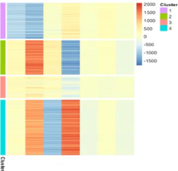
Fig. 10: Usoskin dataset. Heatmap plot of the projected data (XW matrix with ¯d = k + 3 columns; k = 4 for Usoskin dataset). Lines
have been reordered to group the projected samples into classes. The heatmap plot demonstrates that samples in the same cluster do have similar entries.
IV. CONCLUSION
In this paper we focus on unsupervised clustering. We provide a new efficient algorithm based on alternating minimization that achieves feature selection by introducing a ℓ1constraint in the gradient-projection step. This step, of splitting type, uses an exact projection on the ℓ1 ball to promote sparsity, and is alternated with k-means. Convergence of the projection-gradient method is established. Each iterative step of our algorithm necessarily lowers the cost which is so monoton-ically decreasing. The experiments on single-cell RNA-seq dataset in Section III demonstrate that our method is very promising compared to other algorithms in the field. Note that our algorithm can be straightforwardly applied for clustering any high dimensional database (in imaging, social networks, customer relationship management...). Ongoing developments concern the application to very large datasets.
REFERENCES
[1] C. Aggarwal. On k-anonymity and the curse of dimensionality.
Pro-ceedings of the 31st VLDB Conference, Trondheim, Norway, 2005.
[2] D. Arthur and S. Vassilvitski. k-means++: The advantages of careful seeding. Proceedings of the eighteenth annual ACM-SIAM symposium
on Discrete algorithms, 2007.
[3] H. Attouch, J. Bolte, P. Redont, and A. Soubeyran. Proximal alternat-ing minimization and projection methods for nonconvex problems: an approach based on the kurdyka-lojasiewicz inequality. Mathematics of
Operations Research, 2010.
[4] F. R. Bach. Sharp analysis of low-rank kernel matrix approximations.
International Conference on Learning Theory (COLT)., 2013.
[5] F. R. Bach and Z. Harchaoui. Diffrac: a discriminative and flexible framework for clustering. In J. C. Platt, D. Koller, Y. Singer, and S. T. Roweis, editors, Advances in Neural Information Processing Systems 20, pages 49–56. Curran Associates, Inc., 2008.
[6] H. H. Bauschke and P. L. Combettes. Convex Analysis and Monotone
Operator Theory in Hilbert Spaces. Springer, New York, 2011.
[7] A. Beck and M. Teboulle. A fast iterative shrinkage-thresholding algorithm for linear inverse problems. SIAM journal on imaging sciences, 2(1):183–202, 2009.
[8] J. Bolte, S. Sabach, and M. Teboulle. Proximal alternating linearized minimization for nonconvex and nonsmooth problems. Mathematical
Programming, 146(1):459–494, Aug 2014.
[9] L. Bottou and Y. Bengio. Convergence properties of the k-means algorithms. In G. Tesauro, D. S. Touretzky, and T. K. Leen, editors,
Advances in Neural Information Processing Systems 7, pages 585–592.
MIT Press, 1995.
[10] F. Bunea, C. Giraud, M. Royer, and N. Verzelen. PECOK: A convex optimization approach to variable clustering. (1606.05100), 2016. [11] E. J. Candès. The restricted isometry property and its implications for
compressed sensing. Comptes Rendus Acad Sciences Paris, 346(1):589– 592, 2008.
[12] E. J. Candès, M. B. Wakin, and S. P. Boyd. Enhancing sparsity by reweighted ℓ1 minimization. Journal of Fourier analysis and applications, 14(5-6):877–905, 2008.
[13] A. Chambolle and C. Dossal. On the convergence of the iterates of "fista". Journal of Optimization Theory and Applications, Springer Verlag, (166), 2015.
[14] P. L. Combettes and J.-C. Pesquet. Proximal splitting methods in signal processing. In Fixed-point algorithms for inverse problems in science
and engineering, pages 185–212. Springer, 2011.
[15] P. L. Combettes and V. R. Wajs. Signal recovery by proximal forward-backward splitting. Multiscale Modeling & Simulation, 4(4):1168–1200, 2005.
[16] L. Condat. Fast projection onto the simplex and the l1 ball.
Mathemat-ical Programming Series A, 158(1):575–585, 2016.
[17] L. Condat. A convex approach to k-means clustering and image segmentation. HAL, (01504799), 2017.
[18] F. de la Torre and T. Kanade. Discriminative cluster analysis. ICML 06
Proceedings of the 23rd international conference on Machine learning, Pittsburgh, Pennsylvania, USA, 2006.
[19] C. Ding and T. Li. Adaptive dimension reduction using discriminant analysis and k-means clustering. In Proceedings of the 24th International
Conference on Machine Learning, ICML ’07, pages 521–528, New York,
NY, USA, 2007. ACM.
[20] D. L. Donoho and M. Elad. Optimally sparse representation in general (nonorthogonal) dictionaries via ℓ1 minimization. Proceedings of the
National Academy of Sciences, 100(5):2197–2202, 2003.
[21] D. L. Donoho and B. F. Logan. Signal recovery and the large sieve.
SIAM Journal on Applied Mathematics, 52(2):577–591, 1992.
[22] J. Duchi, S. Shalev-Shwartz, Y. Singer, and T. Chandra. Efficient projections onto the l 1-ball for learning in high dimensions. In
Proceedings of the 25th international conference on Machine learning,
pages 272–279. ACM, 2008.
[23] N. Flammarion, B. Palaniappan, and F. R. Bach. Robust discriminative clustering with sparse regularizers. arXiv preprint arXiv:1608.08052, 2016.
[24] T. Hastie, S. Rosset, R. Tibshirani, and J. Zhu. The entire regularization path for the support vector machine. Journal of Machine Learning Research, 5:1391–1415, 2004.
[25] X. He, D. Cai, and P. Niyogi. Laplacian score for feature selection. In Y. Weiss, P. B. Schölkopf, and J. C. Platt, editors, Advances in Neural
Information Processing Systems 18, pages 507–514. MIT Press, 2006.
[26] V. Y. et al Kiselev. Sc3: consensus clustering of single-cell rna-seq data.
Nature Methods, 2017.
[27] A. M. et al Klein. Droplet barcoding for single-cell transcriptomics applied to embryonic stem cells. Cell, 2015.
[28] H. Lawrence and A. Phipps. Comparing partitions. Journal of Classification, 1985.
[29] P.-L. Lions and B. Mercier. Splitting algorithms for the sum of two nonlinear operators. SIAM Journal on Numerical Analysis, 16(6):964– 979, 1979.
[30] J. Mairal and B. Yu. Complexity analysis of the lasso regularization path. In Proceedings of the 29th International Conference on Machine
Learning (ICML-12), pages 353–360, 2012.
[31] D. G. Mixon, S. Villar, and R. Ward. Clustering subgaussian mixtures with k-means. Information and inference, 00:1–27, 2017.
[32] S. Mosci, L. Rosasco, M. Santoro, A. Verri, and S. Villa. Solving structured sparsity regularization with proximal methods. In Machine
Learning and Knowledge Discovery in Databases, pages 418–433.
Springer, 2010.
[33] A. Y. Ng, M. I. Jordan, and Y. Weiss. On spectral clustering: Analysis and an algorithm. In T. G. Dietterich, S. Becker, and Z. Ghahramani, editors, Advances in Neural Information Processing Systems 14, pages 849–856. MIT Press, 2002.
[34] A. P. et al Patel. Single-cell rna-seq highlights intratumoral heterogeneity in primary glioblastoma. Science 344, 2014.
[35] J. Peng and Y. Wei. Approximating k-means-type clustering via semidefinite programming. SIAM J. Optim., 18:186–205, 2017. [36] M. Radovanovic, A. Nanopoulos, and M. Ivanovic. Hubs in space :
Popular nearest neighbors in high-dimensional data. Journal of Machine
Learning Research. 11: 2487?2531.
[37] S. Z. Selim and M. A. Ismail. K-means-type algorithms: A generalized convergence theorem and characterization of local optimality. IEEE Trans. Patt. An. Machine Intel., PAMI-6:81–87, 1984.
[38] S. Sra, S. Nowozin, and S. J. Wright. Optimization for Machine Learning. MIT Press, 2012.
[39] R. Tibshirani. Regression shrinkage and selection via the lasso. Journal
of the Royal Statistical Society. Series B (Methodological), pages 267–
288, 1996.
[40] R. Tibshirani, G. Walther, and T. Hastie. Estimating the number of clusters in a data set via the gap statistic. Journal of the Royal Statistical
Society. Series B (Methodological), pages 411–423, 2001.
[41] D. et al Usoskin. Unbiased classification of sensory neuron types by large-scale single-cell rna sequencing. Nature Neuroscience, 2014. [42] L. J. P. Van der Maaten and G. E. Hinton. Visualizing high-dimensional
data using t-sne. Journal of Machine Learning Research, 9:2579–2605, 2008.
[43] U. Von Luxburg. A tutorial on spectral clustering. Statistics and computing, 2007.
[44] B. Wang, J. Zhu, E. Pierson, D Ramazzotti, and S. Batzoglou. Visualiza-tion and analysis of single-cell rna-seq data by kernel-based similarity learning. Nature methods, (14), 2017.
[45] C. Wei-Chien. On using principal components before separating a mixture of two multivariate normal distributions. Journal of the Royal
Statistical Society, 32(3), 1983.
[46] D. M Witten and R. Tibshirani. A framework for feature selection in clus-tering. Journal of the American Statistical Association, 105(490):713– 726, 2010.
[47] A. et al Zeisel. Cell types in the mouse cortex and hippocampus revealed by single-cell rna-seq. Science, 2015.
Fig. 11: Comparison of 2D visualization using tsne [42]. Each point represents a cell. Misclassified cells in black are reported for 3 datasets : Patel, Klein and Usoskin. K-sparse significantly improves visually the results of Sparcl and SIMLR (note that SIMLR fails to discover a class on Usoskin). This figure shows nice small ball-shaped clusters for K-sparse and SIMLR methods.
![Fig. 11: Comparison of 2D visualization using tsne [42]. Each point represents a cell](https://thumb-eu.123doks.com/thumbv2/123doknet/13048089.382887/10.918.93.779.89.1031/fig-comparison-visualization-using-tsne-point-represents-cell.webp)
