HAL Id: hal-01300086
https://hal.inria.fr/hal-01300086
Submitted on 8 Apr 2016
HAL is a multi-disciplinary open access
archive for the deposit and dissemination of
sci-entific research documents, whether they are
pub-lished or not. The documents may come from
teaching and research institutions in France or
abroad, or from public or private research centers.
L’archive ouverte pluridisciplinaire HAL, est
destinée au dépôt et à la diffusion de documents
scientifiques de niveau recherche, publiés ou non,
émanant des établissements d’enseignement et de
recherche français ou étrangers, des laboratoires
publics ou privés.
Revue Africaine de la Recherche en Informatique et Mathématiques Appliquées, INRIA, 2014, 18,
pp.93-116. �hal-01300086�
RÉSUMÉ. Les techniques d’estimation de canal, basée sur des symboles pilotes, par passage dans un domaine de tranfert sont très attractives pour les systèmes de télécommunications utilisant l’OFDM. Cependant, elles montrent des limites pour les systèmes de télécommunications, où un ensemble de sous-porteuses de garde, est inséré sur les bords du spectre dans le but d’éviter tout recouvre-ment spectral avec d’autres applications utilisant des bandes voisines. Ces sous-porteuses de garde ont selon leur nombre tendance à dégrader fortement les performances de ces estimateurs. Nous proposons, dans un premier temps, une optimisation qui permet d’améliorer considérablement les performances de ces estimateurs quels que soit le nombre de porteuses de garde. Dans un second temps, pour de rendre l’estimateur proposé attractif pour les constructeurs, nous avons proposé une technique permettant de réduire leur complexité de réalisation de manière notable.
ABSTRACT. OFDM based pilots channel estimation methods with processing into the transform do-main appear attractive owing to their capacity to highly reduce the noise component effect. However, in current OFDM systems, null subcarriers are placed at the edge of the spectrum in order to assure isolation from interfering signals in neighboring frequency bands; and the presence of these null car-riers may lead, if not taken into account, to serious degradation of the estimated channel responses due to the “border effect” phenomenon. In this paper an improved algorithm based on truncated SVD is proposed in order to correctly support the case of null carriers at border spectrum. A method for optimizing the truncation threshold whatever the system parameters is also proposed. To make the truncated SVD channel estimation method applicable to any SISO or MIMO OFDM system and what-ever the system parameters, a complexity reduction algorithm based on the distribution of the power in the transfer matrix (based on DFT or DCT) is proposed.
MOTS-CLÉS : systèmes multi porteuses, systèmes multi antennes, Estimation de canal, complexitè, 3GPP/LTE
1. Introduction
The use of orthogonal frequency division multiplexing (OFDM) is now generalized in high data rate wireless communication systems. OFDM benefits from it capacity to mitigate inter-symbol interference (ISI) by adding to the OFDM symbol a time guard in-terval which is longer than the channel impulse response length (or channel delay spread) [1]. Also, frequency-selective channel has been converted to a finite-number of parallel flat channels in the OFDM system owing to the adoption of orthogonal multicarrier tech-nique implemented by fast Fourier transform (FFT). In addition to this, the multicarrier nature of OFDM gives the capability for this technique to overcome the complexity of time equalization method by using a simple frequency equalizer per subcarrier.
In coherent OFDM system, channel estimation has to be performed at the receiver side before the equalization that is carried out in the frequency domain (FD). In some papers, as in [2], authors propose a joint estimation of the channel response and the carrier frequency offsets (CFO). But here we focus only on the channel estimation, as in [3][4][5], and complexity reduction.
In OFDM pilots based channel estimation, that does not require any knowledge of the statistics on the channels, the least square (LS) estimates of the channel response can be obtained by dividing the demodulated pilots signal by the known pilots symbol one in the FD [5]. But the accuracy of the LS estimates is degraded by the noise component. The optimal FD channel estimation technique is minimum mean square error (MMSE) that however needs the information of channel statistic to perform the auto-covariance matrix of the channel frequency response and signal to noise ratio. In addition to this, the associated computation complexity of the MMSE method is very high [6].
Transform domain channel estimation (TD-CE) methods are considered as one of the most promising alternative because it can provide very good results by significantly re-ducing the noise component on the LS estimated channel coefficients obtained in the frequency domain. These methods use discrete fourier transform (DFT) or discrete co-sine transform (DCT). The DFT based method presents the best result in term of noise reduction. However, a “border effect” may occur [7] when null carriers are placed on the spectrum´s extremities in order to assure isolation from interfering signals in neigh-boring frequency bands as well as increasing the sampling frequency. This is a real pro-blem because the vast majority of modern multicarrier systems contain null carriers at the spectrum extremities. Discrete cosine transform (DCT) is suggested instead of DFT for mitigating the impact of the “border effect”, owing to its capacity to reduce the high fre-quency components in the transform domain [5] at the price of a weaker noise reduction [8]. However, when the number of null carriers is important, even the DCT algorithm is not sufficient to reduce significantly the “border effect” [9]. The Karhunen-Loeve trans-form domain algorithm can also be used as in [10] to pertrans-form iteratively the channel smoothing. However the computation complexity of this method is very high.
To correctly support the case of null carriers at border spectrum, an improved algo-rithm based on truncated singular value decomposition (TSVD) of the transform domain matrix is proposed for both DFT and DCT. A method for optimizing the truncation thre-shold whatever the system parameters is also proposed in this paper. This method allows both mitigation of the “border effect” and reduction of the noise component.
The TSVD method presents very good results, but its complexity and latency may cause problems, when the number of subcarrier is large and notably in input multi-output (MIMO) configuration where all the sub-channels between the antenna links have
to be individually estimated. The combination of MIMO and OFDM technologies (MIMO-OFDM) is now largely considered in the new generation of standards for wireless trans-mission [11] because MIMO system has the potential to obtain a diversity gain and to improve the system capacity [12]. Hence channel estimation method with low complexity for MIMO-OFDM system becomes a challenge.
To make the TSVD channel estimation method applicable to MIMO-OFDM system, a complexity reduction algorithm based on the distribution of the power in the trans-fer matrix is proposed in this paper. The efficiency of this algorithm is demonstrated in 3GPP/LTE system context. The output of this paper is also a set of methods allowing the selection and adaptation of the most appropriate TD channel estimation, depending on the system parameters and the complexity/performance requirements.
The paper is organized as follows. Section 2 describes the conventional TD-CE me-thods (DFT and DCT) and its weakness regarding the “border effect”. Then section 3 is dedicated to the TSVD concept and the optimization of the truncated threshold. Next the complexity of the TSVD channel estimation is studied in section 4. The complexity reduction algorithm and its efficiency are detailed in this last section.
2. CLASSICAL TD-CE
The TD-CE based method has been proposed to improve the accuracy of the LS esti-mated channel response which is degraded by the noise component [5][13].
Figure 1. Smoothing process in TD-CE.
The Fig.1 shows the TD-CE smoothing (noise reduction) process. The frequency channel response, estimated by LS channel estimation method, is first converted into the transform domain by a transfer algorithm based on DCT or DFT. Note that the trans-form domain corresponds to the time domain in the case of DFT-based algorithm. Then a smoothing filter is applied, assuming that the useful channel power in this domain is concentrated within the first W samples. For a better understanding, note again that with the DFT-based algorithm, the useful power corresponds to the impulse response of the
channel. After the smoothing, the inverse of the transfer algorithm is applied to return to the frequency domain.
2.1. Comparaison between DFT and DCT
2.1.1. Noise reduction in an ideal context : 2.1.1.1. DFT :
The LS estimate is first converted into the time domain by the IDFT (inverse discrete Fourier transform) algorithm. The time domain channel response of the LS estimated channel can then be given by :
hIDF T n,LS = √ 1 N ∑N−1 k=0 Hk,LSej 2πnk N = hIDF T n + ξnIDF T (1)
where ξnIDF T is the noise component in the time domain and hIDF Tn is the IDFT of
the LS estimated channel without noise.
The baseband time domain of the effective discrete channel response, also called im-pulse response, between the transmit antenna and the receive antenna under the multipath fading environments can be expressed as [6] :
h(n) =
L∑−1 l=0
hlδ(n− τl) (2)
with L the number of paths, hland τlthe complex time varying channel coefficient and
delay of the l-th path.
Therefore, hIDF Tn can be further developed as follows :
hIDF T n = √ 1 N ∑N−1 k=0( ∑L−1 l=0 hle−j 2kπτl N )ej 2πkn N = √ 1 N ∑L−1 l=0 hl ∑N−1 k=0 e−j 2πk N (τl−n) (3)
The last term of (3)∑Nk=0−1e−j2πkN (τl−n)verifies :
N∑−1 k=0 e−j2πkN (τl−n)= { N n = τl 0 otherwise (4) where τl= 0, 1, ..., L− 1 and n = 0, ..., N − 1.
The time domain channel response of the LS estimate hIDF Tn,LS can thus be given by :
hIDF Tn,LS = 1 √ N { N hl=n+ ξnIDF T n = 0, ..., L− 1 ξIDF T n otherwise (5) Assuming W > L, we retrieve the channel taps as well as a reduction of the noise component by applying the smoothing filter of length W :
hIDF Tn,W =√1
N
{
N hl=n+ ξnIDF T n = 0, ..., W− 1
The optimum lenghtfor W is L in order to retrieve all the useful power and maximize the noise reduction. However, as L is not known by the receiver, W is usually set equal to CP (length of the cyclic prefix), which is longer than L in OFDM systems. That is why in the following, the smoothing window size is taken to be equal to CP (W = CP ) [6][13] for DFT based channel estimation.
From (6), it can be observed that the DFT based channel estimation method decreases the noise power level by,
∆(dB) = 10log( N
CP) (7)
After the smoothing process, a DFT algorithm is used to return in the frequency do-main.
2.1.1.2. DCT :
The DCT based channel estimator can be realized by replacing IDFT and DFT by DCT and IDCT respectively [5]. The transform domain channel response can be obtained by the following equation after performing DCT to the LS estimate.
hDCTn,LS = VnN N∑−1 k=0 Hk,LS.cos π(2k + 1)n 2N (8)
where VnN is the coefficient of DCT which can take two different values, depending on
the value of n. VnN = { √ 1/N n = 0 √ 2/N n̸= 0 (9) Similarly to the DFT case, hDCTn,LS can be divided into two parts :
hDCTn,LS = hDCTn + ξnIDCT (10) The DCT method can be considered as the conventional DFT with twice as many points [5][14]. Thus from the multi-path channel characteristics and since the maximum channel taps L is within the cyclic prefix (CP), the transform domain channel response given by (10) would be concentrated in the 2CP first samples of hDCT
n,LS. The noise level
can then be reduced by using a smoothing filter of size W = 2CP and then (6) becomes :
hDCTn,W =
{
hDCT
n,LS 0≤ n ≤ W − 1
0 otherwise (11)
From 11, it can be observed that the DCT based channel estimation method decreases the noise power level by,
∆(dB) = 10log( N
2CP) (12)
From 7 and 12 we can conclude that the DCT based method abducts half as much noise as the DFT method.
2.1.2. “Border effect” in a realistic framework :
In a realistic framework, only a subset of subcarriers (M ) is modulated among the
N due to the insertion of null subcarriers at the spectrum extremities for band isolation
from/to interfering signals that occupy neighboring frequency bands[15] as well as for in-creasing the sampling frequency [16]. The existence of these null subcarriers will directly impact the behavior of the channel estimation in the transform domain.
2.1.2.1. DFT :
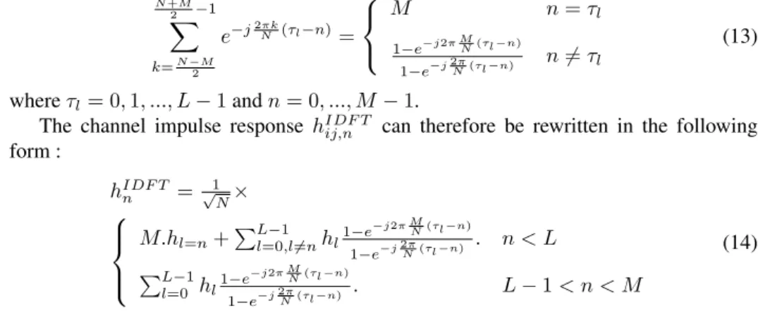
For DFT based channel estimation, when M < N , the expression (4) becomes (see Appendix) : N +M 2 −1 ∑ k=N−M2 e−j2πkN (τl−n)= M n = τl 1−e−j2π MN(τl−n) 1−e−j 2πN(τl−n) n̸= τl (13) where τl= 0, 1, ..., L− 1 and n = 0, ..., M − 1.
The channel impulse response hIDF Tij,n can therefore be rewritten in the following form : hIDF T n = 1 √ N× M.hl=n+ ∑L−1 l=0,l̸=nhl1−e −j2π MN(τl−n) 1−e−j 2πN(τl−n) . n < L ∑L−1 l=0 hl 1−e−j2π MN(τl−n) 1−e−j 2πN(τl−n) . L− 1 < n < M (14)
We can observe that hIDF Tn is no longer concentrated on the first L elements, due to the
phenomenon called “inter-taps interference (ITI)” here. Consequently, by using the smoo-thing filter of length CP in the time domain, part of the useful channel power contained in samples n = CP, ..., M − 1 is lost. This loss of useful power leads to an important degradation regarding the estimation of the channel response. Thus we demonstrate that this phenomenon called “border effect” by Morelli [15] is in fact due to ITI.
2.1.2.2. DCT :
Figure 2. DCT and DFT principle.
DCT can then reduce the component called ITI in the transform domain compared to DFT. An exploration to this is that, for a given sequence of M points, DFT conceptually treats it as a periodic signal with a period of M . Hence, there is an increase of high-frequency components, due to signal discontinuity at the consecutive periods boundary.
In contrast, DCT conceptually extends the original M points sequence to a 2M points sequence by a mirror extension of the M points sequence [14]. As a result, the waveform will be smoother and more continuous in the boundary between consecutive periods (see Fig.2).
Consequently, due to the reduction of the power loss (ITI), the DCT-based algorithm is more robust to “border effect” than the DFT-based one.
2.1.3. MSE performance comparison :
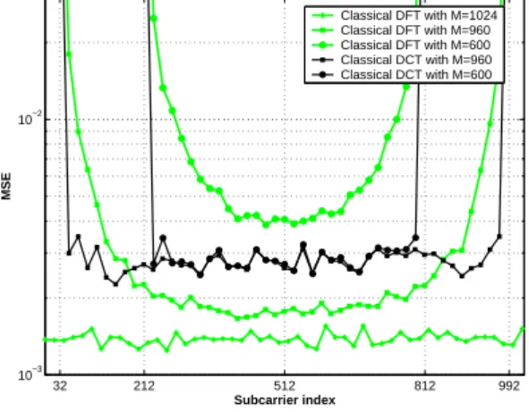
Fig.3 highlights the “border effect” phenomenon by showing the MSE performance on the different subcarriers when applying classical DFT and clasical DCT based channel estimation methods depending on the number of modulated subcarriers. The simulation parameters are listed in Table 3.
Tableau 1. MSE simulation Parameters
Channel Model SCME [17]
Number of FFT points (N) 1024
subcarriers (M) 1024, 960, 600
cyclic prefix 72
Number of Nt& Nrantennas 4 & 2
Bandwidth & Carrier frequency 15.36MHz & 2GHz
Coding Rate 1/3
MIMO scheme double-Alamouti
FEC turbo code (UMTS)
First, when all the subcarriers are modulated (N = M = 1024), there is no “border effect” and the MSE is almost the same for all the subcarriers. This is due to the fact that all the useful channel power is retrieved in the first W samples of the impulse channel response. 32 212 512 812 992 10−3 10−2 Subcarrier index MSE Classical DFT with M=1024 Classical DFT with M=960 Classical DFT with M=600 Classical DCT with M=960 Classical DCT with M=600
Figure 3. Average mean square error versus subcarrier index for classical DFT and
clas-sical DCT based channel estimation. The number of modulated subcarrier are M = 960 and M = 600, N = 1024 and SN R = 10dB.
However when null subcarriers are inserted on the edge of the spectrum (N ̸= M), the MSE performance is degraded and then “border effect” occurs. When the number of null subcarriers is small (M = 960), the DFT based method presents better MSE result in the middle of the bandwidth than the DCT based method. This is due to the fact that DFT abducts more noise than the DCT (see 2.1.1). On the contrary, the DCT performance is better on the edge of the bandwidth due to it capacity to reduce the ITI which causes the “border effect”.
It is already noticeable that the impact of the “border effect” phenomenon in DFT increases obviously with the number of null subcarriers. Thereby, in spite of its weaker noise reduction, DCT presents better result than DFT when the number of null subcarriers is equal to 424 (as in the 3GPP system [16]), i.e M = 600.
2.1.4. Conclusion :
The DFT-based channel estimation suffers in a realistic system from the “border ef-fect” caused by the loss of a part of the useful channel power (the ITI) during the smoo-thing process. The impact of the “border effect” phenomenon increases with the number of null subcarriers. As these ITI are less important in the DCT based method due to it potential to concentrate the useful channel power, it presents better results than the DFT-based method even if it abducts less noise.
Nevertheless, the “border effect” is still present. Thus in order to improve the accuracy of the transform domain channel estimation, it is necessary to both minimize the useful power lost in conventional TD-CE and the noise component.
3. TD-CE WITH MINIMIZATION OF LOST POWER AND NOISE
COMPONENT
In the rest of the paper, we will consider matrix notation in order to facilitate the reading and mathematical demonstrations.
The unitary DFT and DCT matrix T of size N× N can be defined with the following expression : T = 1 1 . . . 1 1 TN(1)(1) . . . TN(2N + 1)(1) .. . ... . . . ... 1 TN(1)(N− 1) . . . TN((2N + 1)(N− 1)) (15) TN(kn) = VnN.cos( π 2N(2k + 1)(n)) for DCT and e−j 2π N×knfor DFT.
To accommodate the null subcarriers at the spectrum extremities, it is necessary to remove the rows of the matrix T corresponding to their positions. Furthermore, in order to take into account the noise reduction in the transform domain described in 2.1.1, we only use the first W columns of T corresponding to the smoothing filter size. Hence the
transfer matrix T becomes :
T′ = T (N− M
2 :
N + M
2 − 1, 1 : W ) (16) where T′is defined, from T , using “Matlab” syntax.
Using this expression, we can rewrite the expression of the classical TD-CE, (1) for DFT and (10) for DCT in a matrix form :
hIDF T ,DCTLS = T′H.HLS (17)
3.1. Existing pseudo inverse approach
3.1.1. Definition :
The pseudo inverse concept is implemented on the DFT based channel estimation with the purpose of reducing the “border effect” phenomenon [18]. The authors consider the following minimization problem :
hpsinvn,LS = arg min
hn
∥T′hn− Hn,LS∥2 (18)
The solution of this minimization problem, the pseudo inverse matrix noted T′†, which is sometimes named the generalized inverse was described by Moore in 1920 in linear
algebra [19]. This technique is often used for the resolution of linear system equations
due to its capacity to minimize the Euclidean norm and then tends towards the exact solution. The pseudo inverse T′†of T′is defined as the unique matrix satisfying all of the four following criteria [20].
1 : T′T′†T′ = T′ 2 : T′†T′T′†= T′† 3 : (T′T′†)H= T′T′† 4 : (T′†T′)H= T†′T′ (19)
We can generalize this technique by applying it to the DFT and DCT based channel estimation. The pseudo inverse solution is then defined as follows :
hDF TLS −psinv,DCT −psinv = (T′HT′)−1T′HHLS= T
′†
HLS (20)
3.1.2. Drawback of the pseudo inverse :
The main problem of the pseudo inverse method is the precision of the inverse calcu-lation which varies depending on the matrix F′. The conditional number of T′, that we call (κ(T′)), is defined as the ratio between the greatest and the smallest singular value of T′. The value of κ(T′) is a good indicator of the inverse precision [16]. The higher
κ(T′) is, the more the estimated channel response is degraded. When all the subcarriers are modulated, κ(T′) = 1 but when null subcarriers are placed at the border of the spec-trum, κ(T′) can become very high. For instance, if N = 1024, M = 960 and CP = 72,
κ(T′) is about 100. However if N = 1024, M = 600 and CP = 72 as in 3GPP, κ(T′) is very high 2.171015and the estimated channel response will be degraded due to the poor
minimization.
3.1.3. Discussion :
Pseudo inverse can minimize the lost power which causes the “border effect” pheno-menon. However the minimization performance depends on the conditional number of the transfer matrix which can be very high in realistic framework as in 3GPP. In order to make the minimization process efficient, we have to reduce the conditional number of the
transfer matrix (κ(T′)) without changing the number of null subcarriers which is imposed by the standard.
In the following approach, we propose the use of SVD decomposition to compute the pseudo inverse matrix. After that we propose a threshold determination which allows the reduction of the conditional number of the transfer matrix by considering only the most significant singular values to further reduce the noise component.
3.2. Channel estimation with truncated SVD
3.2.1. Pseudo inverse computation using SVD :
Applying SVD to the matrix T′, consists in decomposing T′in the following form :
T′ = U SVH (21)
where U ∈ CM×W and V ∈ CM×W are unitary matrices and S∈ CW×W is a diagonal matrix with non-negative real numbers on the diagonal, called singular values.
The pseudo inverse of the matrix T′with singular value decomposition is [19] :
T′†= V S†UH (22)
It is important to note that S†is a diagonal matrix filled with the inverse singular values of T′.
By noting s∈ CW×1the vector which contains the W singular values, we can
calcu-late the conditional number of the matrix T′ as :
κ(T′) =max(s)
min(s) (23)
where max(s) and min(s) give the greatest and the smallest singular value respectively. 3.2.2. Principle and advantages :
3.2.2.1. Principle of TSVD based channel estimation :
Figure 4. Block diagram of transform domain based channel estimation with Truncated
SVD.
To reduce κ(T′), lowest singular values can be eliminated. Hence, any singular value smaller than an optimized threshold (detailed in 3.2.3) is replaced by zero. The principle
is depicted in Fig.4. The matrix S provided by the SV D calculation of the matrix T′ becomes SThwhere This the number of considered singular values.
The channel response after the smoothing window in the transform domain (hT SV DLS of size 1× W ) can thus be expressed as follows :
hT SV DLS = TT′† hHLS= V S † ThU HH LS (24)
Finally T′of size (M× W ) is used to return to the frequency domain.
HT SV D= T′hT SV DLS (25) The TD-CE by TSVD can then be expressed, using the equations (24) and (26), as fol-lows : HT SV D = T′TT′† hHLS= T global Th HLS (26) where TTglobal
h of size M× M represents the global channel estimation matrix. 3.2.2.2. Advantage of TSVD based channel estimation :
Assuming an optimized threshold (3.2.3), the TSVD based channel estimation pre-sents the two following advantages :
(i) On the one hand, the “border effect” is obviously further reduced owing to the re-duction of κ(T′).
(ii) On the other hand, the suppression of the lowest singular values allows the noise component in the estimated channel response to be further reduced. The rank of the ma-trix T′ is W , which means that the useful power of the channel is distributed into W virtual paths with singular values as weightings. The paths corresponding to the lowest singular values will be predominated by noise and their elimination will benefit the noise component reduction.
These theoretical results will be further confirmed by simulation. 3.2.3. How to find the truncated threshold ?
Th (∈ 1, 2, ..., W ) can be viewed as a compromise between the accuracy of the
pseudo-inverse calculation and the conditional number magnitude. An important point is that its value will depend only on the system parameters : the number and position of the modulated subcarriers (M ), the smoothing window size (W ) and the number of FFT points (N ). All these parameters are predefined and are known prior to any chan-nel estimation implementation. It is thus possible to optimize the Th value prior to any
implementation.
To determine a good value of Th, it is important to master its effect on the channel
estimation quality i.e on the global channel estimation matrix TTglobal
h (see equation 24) by respecting the following rules :
(i) When all the singular values of T′ are considered, the conditional number of the global matrix (κ(TTglobal
h )) is very high and the accuracy of the estimated channel response is then degraded by the “border effect”.
(ii) On the contrary, if insufficient singular values are used, the estimated channel res-ponse is also degraded due to a very large power loss, even if the conditional number of
TTglobal
h is minimized.
To assess the optimum value of Thproviding a good compromise between these two
phenomenons, we investigate the behavior of the singular values of TTglobal
0 45 87 144 10−20
10−10 100
Singular value magnitude
DFT DCT
Figure 5. Behavior of the W singular values of the matrix T′ (W = CP for DFT and W = 2CPfor DCT). The system parameters are CP = 72, N = 1024 and M = 600.
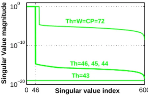
0 46 600
10−20 10−10 100
Singular Value magnitude
Singular value index
Th=46, 45, 44 Th=W=CP=72
Th=43
Figure 6. Behavior of the M singular values of the Global matrix TTglobalh , for several values of Th, when DFT is used. The system parameters are CP = 72, N = 1024 and M = 600.
0 88 600
10−20 10−10 100
Singular value magnitude
Th=88, 87, 86 Th=W=2CP=144
Th=85
Singular value index
Figure 7. Behavior of the M singular values of the Global matrix TTglobalh , for several values of Th, when DCT is used. The system parameters are CP = 72, N = 1024 and M = 600.
Th. Same system parameters are considered : number of FFT points N equal to 1024,
CP = 72 and the number of modulated subcarriers M = 600.
Fig.5 shows all the W singular values of the transfer matrix T′which can be based on the DFT (W = CP = 72) or the DCT (W = 2CP = 144) algorithm. Next, Fig.6 shows also all the M singular values of the global channel estimation matrix TTglobal
h when DFT
is used for several values of Th(72, 46, 45, 44, and 43). Finally Fig.7 shows the behavior
of the M singular values of the global channel estimation matrix when DCT is used for several value of Th(144, 88, 87, 86 and 85).
By considering Th = W for DFT or Th = 2W for DCT, the conditional number of
the transfer matrix T′, which is the ratio between the greatest and the lowest considered singular values, is very high. Hence the conditional number of TTglobal
h is also high (see Fig.5 and Fig.7 when Th= W ).
However, if we reduce the conditional number of the matrix T′ by considering only the most significants Thsingular values (Th = 46, 45 and 44 for DFT and Th = 88, 87
and 86 for DCT), the singular values of TTglobal
h follow a particular form. As we can see , in Fig.6 and Fig.7 when Th= 46, 45 and 44 for DFT and Th= 88, 87 and 86 for DCT,
the the singular values are the same on the first Thindexes and almost null for the other
ones. We can consider that the rank of the matrix TTglobal
h becomes Thinstead of W and that its conditional number is equal to 1 (κ(TTglobal
h ) = 1. Therefore the “border effect” will surely be mitigated and the noise component be minimized.
Nevertheless, as explaining before, we can not indefinitely reduce the value of Th, as
we can see in Fig.6 and Fig.7 when Th≤ 43 for DFT and Th≤ 85, all the singular values
of TTglobal
h become null due to a too large loss of power, even if κ(T ′
) is reduced. 3.2.4. MSE performance :
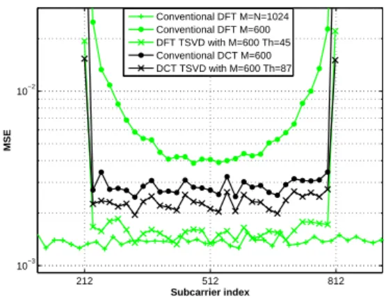
The Fig.8 shows the MSE performance on the different subcarriers when applying classical transform domain channel estimation (DFT and DCT) and truncated SVD me-thod with optimized threshold (Th = 45 for DFT and for DCT Th = 87). The TSVD
method with optimized Thallows the obtention of smaller MSE than with classical
TD-CE on all subcarriers even at the edges of the spectrum. This is due to the optimisation of the TSVD and the reduction of the noise effect provided by the TSVD calculation. We can constat that the DFT TSVD method presents better MSE results than the DCT TSVD one. This is closely related to the length of the smoothing window (W ) which is more important in DCT than in DFT (see 2.1.1).
3.2.5. Conclusion :
The TD-CE with TSVD improves the accuracy of the estimated channel response by mitigating the “border effect” and reducing the noise component. A number of important analysis below are necessary to clarify the algorithm’s properties.
(i) The optimum threshold (Th) needs to be found. As explained previously, its value
depends only on the system parameters which is predefined and known at the receiver side. Therefore the best Thcan be determined in advance by the process illustrated in the
paragraph 3.2.3 and then a global channel estimation matrix TTglobal
h can be pre-computed. (ii) As we can see in 2.1.3, the “border effect” is more important with the DFT based method but it abducts more noise than the DCT one. Therefore the mitigation of this “border effect” by the optimized TSVD makes the DFT-TSVD more efficient than the DCT-TSVD.
212 512 812 10−3 10−2 Subcarrier index MSE Conventional DFT M=N=1024 Conventional DFT M=600 DFT TSVD with M=600 Th=45 Conventional DCT M=600 DCT TSVD with M=600 Th=87
Figure 8. Average mean square error versus subcarrier index for classical DFT, classical
DCT and truncated SVD with optimized threshold based channel estimation. The number of modulated subcarrier are M = 600, N = 1024 and SN R = 10dB.
(iii) The main problem of this method is that the matrix TTglobal
h of size M× M is used. Therefore the complexity and latency of the operation (26) may cause problems, espe-cially in MIMO-OFDM systems where all the subchannels between the antenna links have to be individually estimated. To make these techniques (DFT-TSVD and DCT-TSVD) at-tractive for MIMO-OFDM systems, we have to reduce their complexity. It is important to note that the DFT-TSVD based channel estimation uses complex operations while DCT-TSVD uses real operations. Thus the complexity of DCT-TSVD based channel estimation is more important in DFT even if it presents better results than the DCT. A trail of com-plexity reduction is to make a profit on the fact that the κ(TTglobal
h ) = 1 by studying the distribution of power around the diagonal of TTglobal
h . A complexity reduction method is proposed in the following section.
4. COMPLEXITY REDUCTION IN MIMO-OFDM SYSTEM
4.1. Complexity of the truncated SVD
Considering a MIMO-OFDM system with Nttransmit antennas and Nrreceived ones,
the global matrix TTglobal
h is used Nt× Nrtimes to estimate the MIMO channel between all the antenna links. The operation HT SV D= TTglobal
h HLS, from equation (26), requires
M× M complex multiplications1and 2M× (M − 1) complex additions2in DFT based method. The DFT uses complex operations whereas the DCT uses real ones. Thereby, in DCT based method, there are only operations3between real and complex coefficients.
The conclusion, in terms of complexity, is the same for DFT and DCT based method : the complexity of the channel estimation can be very high, when the number of
subcar-1. (a + jb)(c + jd) = (ac− bd) + j(ad + bc) : 4 real multiplications and 2 real additions 2. (a + jb) + (c + jd) = (a + c) + j(b + d) : 2 real additions
Tableau 2. Number of real multiplications and real additions necessary for the estimation
of the MIMO channel between all the Nt× Nrantenna links.
Transform domain Real multiplications Real additions algorithm
DFT (4M2)× N
t× Nr (2M2+ 2M× (M − 1)) × Nt× Nr
DCT (2M2)× N
t× Nr (2M× (M − 1)) × Nt× Nr
rier is large and notably in MIMO configuration where all the sub-channels between the antenna links have to be individually estimated (see Table.2).
4.2. Complexity reduction
4.2.1. Trail of the complexity reduction :
In section 3.2.2 we saw that the global channel estimation TTglobal
h is perfectly condi-tioned, i.e κ(TTglobal
h ) = 1 for optimized Th. This has a direct impact on the localization of the power in the matrix TTglobal
h . The most significant values in the global matrix are concentred around its diagonal. In order to reduce the complexity of the channel estima-tion, we can only take into account the elements which are around the diagonal of the global matrix.
4.2.2. Complexity reduction :
To reduce the complexity of the MIMO channel estimation, we only use D among the
M elements in each row of the matrix TTglobalh of size M×M. The principle is represented in the Fig.9 where⌈D/2⌉ means ceil of D/2. Fig.10 represents the percentage of power kept by using different values for D where N = 1024, CP = 72 and M = 600. As we can see, D = 4 and D = 8 are sufficient to achieve more than 90% of the total power in TTglobal
h for DCT and DFT respectively. We can note that DCT algorithm better concentrates the power around the diagonal than DFT. This point constitutes the great interest in DCT.
Nevertheless, the choice of D induces a tradeoff between the accuracy of the proposed channel estimation scheme and its complexity :
(i) On the one hand, the lower D, the lower the complexity. Table 4 shows the compari-son between the conventional TD-CE with optimized threshold (see 26) and the proposed complexity reduction scheme (see Fig.9) in terms of the number of required real multipli-cations and real additions. The DFT uses complex operations whereas the DCT uses real ones. Therefore the complexity of the proposed scheme is less important for DCT than for DFT.
(ii) On the other hand, the lower D is, the more the accuracy of the proposed channel estimation scheme is affected.
As seen in the subsection 2.1.3, the DFT is very sensitive to a loss of power. Therefore the “border effect” can reappear when the value of D is low. On the contrary, the DCT is robust against a loss of useful power. In addition to that, it better concentrates the power than the DFT (see Fig 10). Thus this technique will be better adapted to DCT.
D
M
(D/2)
Figure 9. Representation of the D used elements of Tglobal
Th .
4.3. Application
The performance of the DFT and DCT based channel estimation methods with optimi-zed threshold Thand the complexity reduction scheme detailed in this paper are evaluated
in the 3GPP/LTE (typical outdoor) system environments (downlink transmission). 4.3.1. Systems parameters :
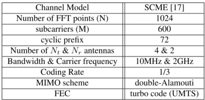
The simulation parameters are listed in Table 3. 4.3.2. Simulation result :
Perfect time and frequency synchronizations are assumed. Monte Carlo simulation results in term of bit error rate (BER) versus Eb
N0 are presented here for the different
chan-nel estimation methods : DFT and DCT with optimized Thand the complexity reduction
scheme (several value of D). The value of Eb
N0 can be inferred from the signal to noise
ratio (SNR) : Eb N0 = Nt mRcRM .σ 2 s σ2 n = Nt mRcRM .SN R (27) where σ2
noiseand σx2represent the noise and signal variances respectively. Rc, RMand m
represent the coding rate, the MIMO scheme rate and the modulation order respectively.
4 8 20 40 60 72 82 84 86 88 90 92 94 96 98 100 99
Number of diagonal elements D
Power percentage
DCT−Th=87 DFT−Th=45
Tableau 3. Simulation Parameters
Channel Model SCME [17]
Number of FFT points (N) 1024
subcarriers (M) 600
cyclic prefix 72
Number of Nt& Nrantennas 4 & 2
Bandwidth & Carrier frequency 10MHz & 2GHz
Coding Rate 1/3
MIMO scheme double-Alamouti
FEC turbo code (UMTS)
Fig.11 and Fig.12 show the performance results in terms of BER versusEb
N0 for perfect,
DFT and DCT with optimized Thand the complexity reduction scheme based channel
estimation in 3GPP/LTE environment where 16QAM and 64QAM are respectively used. 4.3.2.1. DFT and DCT with optimized threshold :
DCT and DFT with optimized threshold (DCT-Th=87 and DFT-Th=45) improve the BER performance compared to the least square one (LS). This is due to the transform domain processing. In 3GPP context, the number of null subcarriers at the edge of the spectrum which can create “border effect” is very important (424). However the opti-mization of the truncated singular value decomposition allows to mitigate this “border effect” and then to benefit from the noise component reduction. Nevertheless, the DFT based method which abducts more noise than the DCT (Th= 87 > Th= 45) based one,
presents better BER performance.
4.3.2.2. Proposed complexity reduction scheme :
The proposed complexity reduction based method, which consists of the use of some diagonals of the global transfer matrix, is more adapted to the DCT. 90% of the total power in the global transfer matrix (D = 4 see Fig.10) is enough to have no degradation of performance when 16QAM modulation is used. On the contrary, the DFT which is very sensitive to a loss of power presents an error floor when D = 4 or D = 8 (90% or 95% of the total power). It needs 99% (D = 72) of the total power to achieve a similar performance to the proposed DCT one (see Fig.11).
When 64QAM modulation is used, power loss sensitivity increases and then DFT with the proposed complexity reduction scheme presents poor performance, worse than the LS one, even if 99% of the total power is considered (see Fig.12). Nevertheless the DCT based method resists very well, but 95% of the total power (D = 8) is needed instead of 90% (D = 4) for 16QAM modulation.
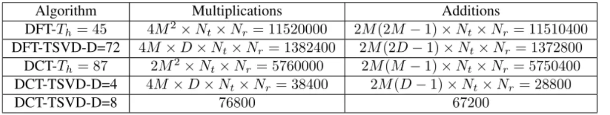
Table (4) contains the number of required real operations to estimate the Nt×Nr
sub-channels. As we can see, the complexity of the proposed scheme with the DCT algorithm is very low compared to the others techniques. Note also that the DFT based method re-quires more operations (36 times) in order to achieve the same performance result when 16QAM modulation is used.
2 3 4 5 6 7 8 10−4 10−3 10−2 10−1 100 Eb/No BER Perfect LS DFT−Th=45 DFT−TSVD−D4 DFT−TSVD−D8 DFT−TSVD−D72 DCT−Th=87 DCT−TSVD−D4
Figure 11. BER versus Eb
N0 for perfect, least square (LS), DFT with optimized Th = 45, DCT with optimized Th= 87, DFT with complexity reduction scheme DF T−T SV D−D =
4, 8, 72and DCT with complexity reduction scheme DF T−T SV D −D = 4 based channel estimation where 16QAM modulation is used in 3GPP environment. Nt = 4, Nr = 2, N = 1024, CP = 72 and M = 600. 5 6 7 8 9 10 11 10−4 10−3 10−2 10−1 100 Eb/No BER PerfectLS DFT−Th=45 DFT−TSVD−−D4 DFT−TSVD−D8 DFT−TSVD−D72 DCT−Th=87 DCT−TSVD−D4 DCT−TSVD−D8
Figure 12. BER versusEb
N0 for perfect, least square (LS), DFT with optimized Th= 45, DCT with optimized Th = 87, DFT with complexity reduction scheme DF T − T SV D − D =
4, 8, 72and DCT with complexity reduction scheme DF T − T SV D − D = 4, 8 where
64QAM modulation is used in 3GPP environment. Nt= 4, Nr = 2, N = 1024, CP = 72 and M = 600.
Tableau 4. Number of required real operations to estimate the Nt×Nrsubchannels (Nt=
4,Nr= 2)
Algorithm Multiplications Additions
DFT-Th= 45 4M2× Nt× Nr= 11520000 2M (2M− 1) × Nt× Nr= 11510400
DFT-TSVD-D=72 4M× D × Nt× Nr= 1382400 2M (2D− 1) × Nt× Nr= 1372800
DCT-Th= 87 2M2× Nt× Nr= 5760000 2M (M− 1) × Nt× Nr= 5750400
DCT-TSVD-D=4 4M× D × Nt× Nr= 38400 2M (D− 1) × Nt× Nr= 28800
DCT-TSVD-D=8 76800 67200
(i) the complexity reduction scheme is perfectly filled for DCT as it gains the same performance as the DCT with optimized threshold and a lower complexity (150 times for 16QAM and 75 times for 64QAM ). DCT with complexity reduction is therefore very attractive for MIMO-OFDM system due to its improved performance (almost 1.5dB gain compared to LS) and its very low complexity.
(ii) the complexity reduction scheme is degraded too strong for the performance of DFT. It is therefore better to prioritize performance for DFT based channel estimation as the DFT with optimized threshold presents the best results whatever the modulation (16QAM or 64QAM ). This solution will be perfectly suited to devices that can afford important complexity.
5. CONCLUSION
Transform domain channel estimation has been investigated in this paper regarding SISO-OFDM and MIMO-OFDM system environment. The key system parameter, taken into account here, is the number of null carriers at the spectrum extremities which are used on the vast majority of multicarrier systems. Conditional number magnitude of the transform domain matrix has been shown as a relevant metric to gauge the degradation on the estimation of the channel response. The limit of the conventional DFT and DCT tech-niques has been demonstrated by increasing the number of null subcarriers which directly generates a high conditional number. A concept named truncated SVD has been proposed to completely eliminate the impact of the null subcarriers whatever their number. A tech-nique which allows the determination of the truncation threshold for any SISO-OFDM or MIMO-OFDM system is also proposed. DCT and DFT with this optimized threshold improve the performance compared to the conventional one. Due to the complete elimi-nation of the impact of nullcarriers, also called “border effect”, the DFT based method which abducts more noise than the DCT based one, presents better performance.
The complexity of the proposed truncated SVD based channel estimation has been studied for DFT and DCT. It has been shown that the complexity can be very high when the number of subcarriers is large and notably in (MIMO) configuration. Hence, a com-plexity reduction method based on the power profile of the transform domain matrix has been proposed. This complexity reduction scheme perfectly fits the DCT as it does not impact the performance of the DCT with optimized threshold. However, it has been shown that it degrades too strong the performance of the DFT based method.
The choice between these channel estimation scheme (DFT and DCT based method) will depend on the system parameters and the computing complexity that the devices can afford. The DCT with the proposed complexity reduction scheme can be used in order to have a good tradeoff between performance and complexity while the DFT with optimized
truncation threshold is perfectly suited to devices that can afford important complexity or for system parameters leading to fewer computing operation.
Appendix
Demonstration of equation (14).
The channel impulse response described in (3) can be developed as following expres-sion when M < N . hIDF Tn = √ 1 N ∑N +M 2 −1 k=N−M2 ( ∑L−1 l=0 hle−j 2πτlk N )e−j 2πkn N = √ 1 N ∑L−1 l=0 hl ∑N +M 2 −1 k=N−M2 e −j2πk(τ l−n) (28) – When n = τl, N +M 2 −1 ∑ k=N−M2 e−j2πkN (τl−n) = N +M 2 −1 ∑ k=N−M2 1 = M (29)
– When n̸= τl, the last term of (28)
∑N +M 2 −1 k=N−M2 e −j2πk N (τl−n)is a sum of M numbers (e−j2πkN (τl−n), k = N−M 2 , ..., N +M
2 − 1) in a geometric progression and then :
N +M 2 −1 ∑ k=N−M2 e−j2πkN (τl−n)= 1− e −j2πM N(τl−n) 1− e−j2πN(τl−n) (30)
From 29 and 30, the expression (14) is demonstrated. ∑N +M 2 −1 k=N−M2 e −j2πk N (τl−n)= M n = τl 1−e−j2π MN(τl−n) 1−e−j 2πN(τl−n) n̸= τl
6. References
[1] F.DACOSTAPINTO, F.S.O. SCORALICK, F.P.V. DECAMPOS, Z. QUAN AND M.V. RI
-BEIRO, « A low cost OFDM based modulation schemes for data communication in the passband
frequency », IEEE International Symposium on Digital Object Identifier, vol. 424-429, 2011. [2] B. AZIZ, I. FIJALKOW ANDM. ARIAUDO, « JOINT ESTIMATION OF CHANNEL AND
CARRIER FREQUENCY OFFSET FROM THE EMITTER, IN AN UPLINK OFDMA SYS-TEM », IEEE ICASSP 2011, vol. 3492-3495, 2011.
[3] LIU, Y. ; TAN, Z. ; HU, H. ; CIMINI, L.J. ; YELI, G., « Channel estimation for OFDM »,
Communications Surveys and Tutorials, IEEE, vol. 2014.
[4] XU, P. ; WANG, J. ; WANG, J. ; QI, F., « Analysis and Design of Channel Estimation in Multi-cell Multi-user MIMO OFDM Systems », IEEE Transactions on Vehicular Technology, vol. 2014.
[5] S. FENG; N. HU; B. YANG AND W. WU, « DCT-Based Channel Estimation Method for MIMO-OFDM Systems », IEEE WCNC, vol. 3, 2007.
[6] J. VAN DEBEEK, O. EDFORS, M. SANDELL, S. K. WILSON ANDP. O. BORJESSON, « On Channel Estimation in OFDM Systems », IEEE VTC, vol. 2, 1995.
[7] E. G. LARSSON,AND J. LI, « Preamble Design for Multiple-Antenna OFDM-based WLANs with Null Subcarriers », IEEE Signal Processing Letters, vol. 8, 2001.
[8] M. DIALLO, L. BOHER, R. RABINEAU, L. CARIOU ANDM. HELARD, « Transform Domain Channel Estimation with null Subcarriers for MIMO-OFDM systems », IEEE ISWCS, 2008.
[9] M. DIALLOR. RABINEAU ANDL. CARIOU, « Robust DCT based Channel Estimation for
MIMO-OFDM systems », IEEE WCNC, 2009.
[10] E. JAFFROT, M. SIALA, « Turbo channel estimation for OFDM systems on highly time and frequency selective channels », IEEE ICASSP, vol. 5,2977-2980, 2000.
[11] N. BOUBAKER, K. B. LETAIEF AND R. D. MURCH, « A low complexity multi-carrier
BLAST architecture for realizing high data rates over dispersive fading channels », IEEE VTC, vol. 2, 2001.
[12] I. E. TELATAR, « Capacity of Multi-antenna Gaussien Channel », ATT Bell Labs tech.memo, , 1995.
[13] Y. ZHAO ANDA. HUANG, « A Novel Channel Estimation Method for OFDM Mobile
Com-munication Systems Based on Pilot Signals and Transform-Domain Processing », IEEE VTC, vol. 47, 1997.
[14] Y. ZHAO ANDA. HUANG, « Communication Audiovisuelle », Springer, , 2003.
[15] M. MORELLI ANDU. MENGALI, « A comparison of pilot-aided channel estimation methods for OFDM systems », IEEE Transactions on Signal Processing, vol. 49, 2001.
[16] M. MORELLI ANDU. MENGALI, « : E-UTRA and E-UTRAN overall description », 3GPP
TS 36.300 V8.4.0, , 2008.
[17] A. B. WATSON, « Image Compression Using the Discrete Cosine Transform », Mathematica
Journal, , 1994.
[18] X.G. DOUKOPOULOS ANDR. LEGOUABLE, « Robust Channel Estimation via FFT Interpo-lation for Multicarrier Systems », IEEE VTC, , 2007.
[19] E. H. MOORE, « On the reciprocal of the general algebraic matrix », Bulletin of the American
Mathematical Society, vol. 26, 1920.
[20] R. PENROSE, « A generalized inverse for matrices », Proceedings of the Cambridge
Philo-sophical Society, vol. 51, 1955.
[16] R. PENROSE, « Componentwise Condition Numbers for Generalized Matix Inversion and
Linear least sqares », AMS subject classification, , 1991.
[17] D. S. BAUM, J. HANSEN, D. DELGALDO, M. MILOJEVIC, J. SALO ANDP. KY ¨0STI, « An interim channel model for beyond-3g systems : extending the 3gpp spatial channel model (smc) », IEEE VTC, vol. 5, 2005.