A machine learning filter for the slot filling task
Texte intégral
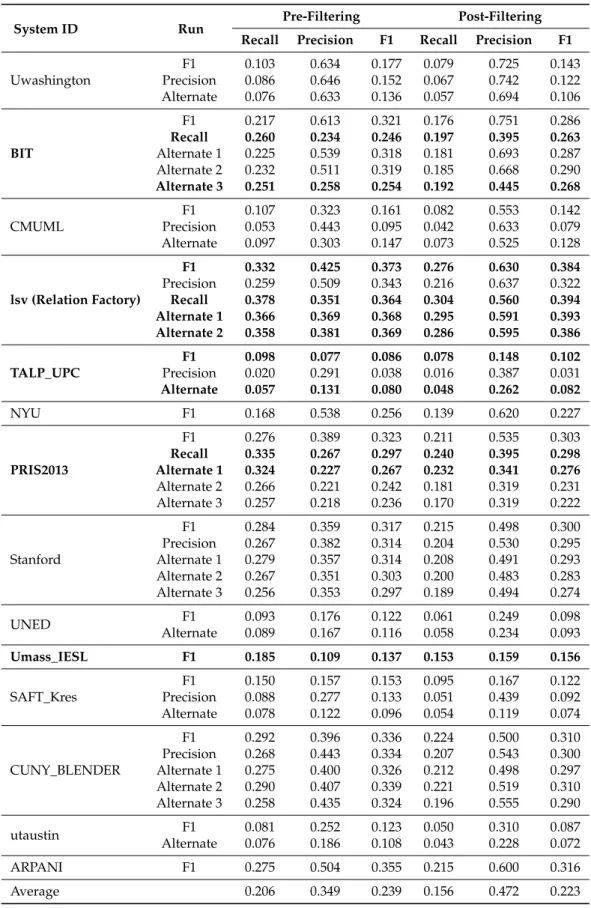
Figure

![Table 1. List of 41 pre-defined relations in TAC KBP 2013 English Slot Filling track and their categorization [24].](https://thumb-eu.123doks.com/thumbv2/123doknet/8193365.275140/7.892.144.756.323.1055/table-list-defined-relations-english-slot-filling-categorization.webp)


Documents relatifs
We present in this section the model and the processing of the MIMO STAP data using firstly conventional approach and secondly multidimensional approach based on the AU- HOSVD. We
The purpose of the present paper is to study the stability of the Kalman filter in a particular case not yet covered in the literature: the absence of process noise in the
It is shown in this paper that the uniform complete observability alone is sufficient to ensure the asymptotic stability of the Kalman filter applied to time varying output
It is shown in this paper that the uniform complete observability is sufficient to ensure the stability of the Kalman filter applied to time varying output error systems, regardless
La Session 1 a concerné « Les nouveaux outils expérimentaux et de simulation pour la conception, la synthèse et la formulation de matériaux ».. Cette session a mis en exergue d
(a) Example in training set 1: handwriting image after removing the discrete printed text com- ponents, (b) Example in training set 2: image with handwriting components except for
Les infestations de la variété Portugaise par la cochenille noire en fonction des directions de l‟arbre montre qu‟en 2012-2013 les dégâts sont plus importants qu‟en 2014.
We fo- cus on a large pollution plume encountered over the east- ern Mediterranean between 1 and 12 August originating in South Asia (India and Southeast Asia), referred to as the
