arXiv:1508.07027v1 [astro-ph.EP] 27 Aug 2015
R.A. StreetR1, A. UdalskiO1, S. Calchi NovatiS1,S2,S3,a, M.P.G. HundertmarkR2, W. ZhuS4, A. GouldS4, J. YeeS5,b, Y. TsaprasR3, D.P. BennettM 1
and
The RoboNet Project & MiNDSTEp Consortium,
U. G. JørgensenR2, M. DominikR4,c, M.I. AndersenR6, E. BacheletR1,R7, V. BozzaS2,R8, D. M. BramichR7, M. J. BurgdorfR9, A. CassanR10, S. CiceriR11, G. D’AgoS3, Subo DongR12, D. F. EvansR13 Sheng-hong GuR14, H. HarkonnenR2, T. C. HinseR15, Keith HorneR4, R. Figuera JaimesR4,R16, N. KainsR17, E. KerinsR17, H. KorhonenR19,R6, M. KuffmeierR2, L. ManciniR11, J. MenziesR20, S. MaoR21, N. PeixinhoR22, A. PopovasR2, M. RabusR23,R11, S. RahvarR24, C. RancR10, R. Tronsgaard RasmussenR25, G. ScarpettaS3,S2, R. SchmidtR3, J.
SkottfeltR26, C. SnodgrassR27, J. SouthworthR13, I.A. SteeleR28, J. SurdejR29, E. Unda-SanzanaR22, P. VermaS3, C. von EssenR25, J. WambsganssR3, Yi-Bo. WangR14, O.
WertzR29 and
The OGLE Project,
R. PoleskiS4,O1, M. PawlakO1, M.K. Szyma´nskiO1, J. SkowronO1, P. Mr´ozO1, S. Koz lowskiO1, L. WyrzykowskiO1, P. PietrukowiczO1, G. Pietrzy´nskiO1, I. Soszy´nskiO1, K. UlaczykO2,
and
The Spitzer Team,
C. BeichmanS1, G. BrydenS6, S. CareyS7, B. S. GaudiS4, C. HendersonS4, R. W. PoggeS4, Y. ShvartzvaldS6,d
and
The MOA Collaboration,
F. AbeM 2, Y. AsakuraM 2, A. BhattacharyaM 1, I.A. BondM 3, M. DonachieM 4, M. FreemanM 4, A. FukuiM 5, Y. HiraoM 6, K. InayamaM 7, Y. ItowM 2, N. KoshimotoM 6,
M.C.A. LiM 4, C.H. LingM 3, K. MasudaM 2, Y. MatsubaraM 2, Y. MurakiM 2, M. NagakaneM 6, T. NishiokaM 2, K. OhnishiM 8, H. OyokawaM 2, N. RattenburyM 4, To. SaitoM 9, A. SharanM 4, D.J. SullivanM 10, T. SumiM 6, D. SuzukiM 2, P.,J. TristramM 11,
and
KMTNet Modeling Team,
C. HanK1, J.-Y.ChoiK1, H. ParkK1, Y. K. JungK1, I.-G. Shin,K1 R1LCOGT, 6740 Cortona Drive, Suite 102, Goleta, CA 93117, USA O1Warsaw University Observatory, Al. Ujazdowskie 4, 00-478 Warszawa,Poland S1NASA Exoplanet Science Institute, MS 100-22, California Institute of Technology,
Pasadena, CA 91125, USA
S2Dipartimento di Fisica ”E.R. Caianiello”, Universit`a di Salerno, Via Giovanni Paolo II 132, 84084, Fisciano, Italy
S3Instituto Internazionale per gli Alti Studi Scientifici (IIASS), Via G. Pellegrino 19, 84019 Vietri sul Mare (SA), Italy
R2Niels Bohr Institute & Centre for Star and Planet Formation, University of Copenhagen, Øster Voldgade 5, 1350 - Copenhagen K, Denmark
S4Department of Astronomy, Ohio State University, 140 W. 18th Ave., Columbus, OH 43210, USA
S5Harvard-Smithsonian Center for Astrophysics, 60 Garden St., Cambridge, MA 02138, USA ; Sagan Fellow.
R3Astronomisches Rechen-Institut, Zentrum f¨ur Astronomie der Universit¨at Heidelberg (ZAH), 69120 Heidelberg, Germany
M 1Department of Physics, University of Notre Dame, Notre Dame, IN 46556, USA R4SUPA, School of Physics & Astronomy, University of St Andrews, North Haugh, St
Andrews KY16 9SS, UK
R5Astronomisches Rechen-Institut, Zentrum f¨ur Astronomie der Universit¨at Heidelberg (ZAH), 69120 Heidelberg, Germany
R6Niels Bohr Institute & Dark Cosmology Centre, University of Copenhagen, Juliane Mariesvej 30, 2100 - Copenhagen Ø, Denmark
R7Qatar Environment and Energy Research Institute, Qatar Foundation, P.O. Box 5825, Doha, Qatar
R9Meteorologisches Institut, Universit¨at Hamburg, Bundesstraße 55, 20146 Hamburg, Germany
R10Sorbonne Universit´es, UPMC Univ Paris 6 et CNRS, UMR 7095, Institut d’Astrophysique de Paris, 98 bis bd Arago, 75014 Paris, France
R11Max Planck Institute for Astronomy, K¨onigstuhl 17, 69117 Heidelberg, Germany R12Kavli Institute for Astronomy and Astrophysics, Peking University, Yi He Yuan Road 5,
Hai Dian District, Beijing 100871, China
R13Astrophysics Group, Keele University, Staffordshire, ST5 5BG, UK R14Yunnan Observatories, Chinese Academy of Sciences, Kunming 650011, China R15Korea Astronomy & Space Science Institute, 776 Daedukdae-ro, Yuseong-gu, 305-348
Daejeon, Republic of Korea
R16European Southern Observatory, Karl-Schwarzschild Straße 2, 85748 Garching bei M¨unchen, Germany
R17Space Telescope Science Institute, 3700 San Martin Drive, Baltimore, MD 21218, United States of America
R18Jodrell Bank Centre for Astrophysics, School of Physics and Astronomy, University of Manchester, Oxford Road, Manchester M13 9PL, UK
R19Finnish Centre for Astronomy with ESO (FINCA), V¨ais¨al¨antie 20, FI-21500 Piikki¨o, Finland
R20South African Astronomical Observatory, PO Box 9, Observatory 7935, South Africa R21National Astronomical Observatories, Chinese Academy of Sciences, 100012 Beijing,
China
R22Unidad de Astronom´ıa, Fac. de Ciencias B´asicas, Universidad de Antofagasta, Avda. U. de Antofagasta 02800, Antofagasta, Chile
R23Instituto de Astrof´ısica, Facultad de F´ısica, Pontificia Universidad Cat´olica de Chile, Av. Vicu˜na Mackenna 4860, 7820436 Macul, Santiago, Chile
R24Department of Physics, Sharif University of Technology, PO Box 11155-9161 Tehran, Iran
R25Stellar Astrophysics Centre, Department of Physics and Astronomy, Aarhus University, Ny Munkegade 120, DK-8000 Aarhus C, Denmark
R26Centre for Electronic Imaging, Department of Physical Sciences, The Open University, Milton Keynes, MK7 6AA, UK
R27Planetary and Space Sciences, Department of Physical Sciences, The Open University, Milton Keynes, MK7 6AA, UK
R28Astrophysics Research Institute, Liverpool John Moores University, Liverpool CH41 1LD, UK
R29Institut d’Astrophysique et de G´eophysique, All´ee du 6 Aoˆut 17, Sart Tilman, Bˆat. B5c, 4000 Li`ege, Belgium
O2Department of Physics, University of Warwick, Gibbet Hill Road, Coventry, CV4 7AL, UK
S6Jet Propulsion Laboratory, California Institute of Technology, 4800 Oak Grove Drive, Pasadena, CA 91109, USA
S7Spitzer, Science Center, MS 220-6, California Institute of Technology,Pasadena, CA, USA
M 2Solar-Terrestrial Environment Laboratory, Nagoya University, Nagoya 464-8601, Japan M 3Institute of Information and Mathematical Sciences, Massey University, Private Bag
102-904, North Shore Mail Centre, Auckland, New Zealand
M 4Department of Physics, University of Auckland, Private Bag 92019, Auckland, New Zealand
M 5Okayama Astrophysical Observatory, National Astronomical Observatory of Japan, 3037-5 Honjo, Kamogata, Asakuchi, Okayama 719-0232, Japan
M 6Department of Earth and Space Science, Graduate School of Science, Osaka University, Toyonaka, Osaka 560-0043, Japan
M 7Department of Physics, Faculty of Science, Kyoto Sangyo University, 603-8555 Kyoto, Japan
M 8Nagano National College of Technology, Nagano 381-8550, Japan M 9Tokyo Metropolitan College of Aeronautics, Tokyo 116-8523, Japan
M 10School of Chemical and Physical Sciences, Victoria University, Wellington, New Zealand
M 11Mt. John University Observatory, P.O. Box 56, Lake Tekapo 8770, New Zealand K1Department of Physics, Chungbuk National University, Cheongju 361-763, Republic of
Korea
aSagan Visiting Fellow bSagan Fellow
cRoyal Society University Research Fellow dNASA Postdoctoral Program Fellow
ABSTRACT
We report the detection of a Cold Neptune mplanet = 21 ± 2 M⊕ orbiting a 0.38 M⊙ M dwarf lying 2.5–3.3 kpc toward the Galactic center as part of a cam-paign combining ground-based and Spitzer observations to measure the Galactic distribution of planets. This is the first time that the complex real-time protocols described by Yee et al. (2015a), which aim to maximize planet sensitivity while maintaining sample integrity, have been carried out in practice. Multiple survey and follow-up teams successfully combined their efforts within the framework of these protocols to detect this planet. This is the second planet in the Spitzer Galactic distribution sample. Both are in the near-to-mid disk and clearly not in the Galactic bulge.
Subject headings: gravitational lensing: micro
1. Introduction
The 2015 Spitzer microlensing campaign is the first project with the specific goal of characterizing the Galactic distribution of planets. Such characterization has three require-ments:
1) A survey that is sensitive to planets in substantially different Galactic environments. 2) Well-characterized selection.
3) Ability to determine, at least statistically, the Galactic environment of each potential host, whether a planet is detected or not.
At present, microlensing is the only possible method to attack this problem because all other planet search techniques fail criterion (1). By contrast, microlensing is about equally sensitive to planet-hosting lenses at all distances along the line of sight from the Sun to the Galactic-bulge sources that are monitored for microlensing events.
Initially microlensing planet searches were conducted in a fairly opportunistic way, dom-inated by targeted follow-up of “interesting” events. Because “interesting” was not neces-sarily well-defined, it was difficult to satisfy criterion (2). Nevertheless Gould et al. (2010) and Cassan et al. (2012) were able to construct subsamples with well-characterized selec-tion. In parallel, the RoboNet and MiNDSTEp teams developed robotic algorithms (Horne Tsapras & Snodgrass 2009; Dominik et al. 2010; Hundertmark et al. 2015) to carry out the target selection in a repeatable and well-characterized manner. With the advent of second generation surveys, particularly OGLE-IV and KMTNet, uniform selection is becoming rou-tine (see, e.g. Suzuki et al. 2015; Shvartzvald et al. 2015). In their high-cadence zones, these wide field surveys can obtain dense enough coverage that additional follow-up observa-tions are not necessary to detect and characterize planets. Hence, events can be monitored uniformly with a pre-defined observing sequence.
The main problem has always been to determine the location of the lenses that are being probed for planets, including both those in which planets are detected and those for which they are not. For the great majority of microlensing events, the lens (host) star is not definitively identified and for many it is not detected at all. For these cases, the microlens parallax πE≡ πrel θE µ µ; θ 2 E≡ κMπrel; κ ≡ 4G c2AU ≃ 8.1 mas M⊙ , (1)
is the key to determining the lens mass and distance. Here, πrel = AU(D−1L − D−1S ) and µ are respectively the lens-source relative parallax and proper motion, θE is the angular Einstein radius, and M is the lens mass. As detailed by Figure 1 from Gould & Horne (2013), the amplitude πE= πrel/θE is set by the fact that motion by the observer of 1 AU displaces the apparent angular separation of the lens and source by an angle πrel, which in turn induces microlensing effects according to how large this displacement is compared to the Einstein radius. In principle, there are two ways to observe the displacement caused by parallax. First, the observer can wait to be moved by Earth’s orbital motion, creating a displacement relative to simple rectilinear motion between the source and lens. Second, two observers at substantially different locations can compare their observations.
Some microlens parallaxes have been measured from the ground using the first effect, particularly for long timescale events (Poindexter et al. 2005) and including fortuitously a significant number of microlens planetary events (Gould et al. 2010). However, the sample of events with parallaxes measured from the ground is extremely heavily biased toward nearby
lenses because they have projected Einstein radii ˜rE ≡ AU/πE ∼ 2–5 AU, roughly 3 times smaller than is typical of bulge lenses. Hence, this sample is almost unusable for measuring the Galactic distribution of planets
The alternative is space-based parallaxes. At ∼ 1 AU from Earth, Spitzer is ideally located to be such a “microlens parallax satellite”. It does, however, face a number of challenges. First, due to Sun-angle viewing restrictions, it can observe Galactic bulge targets (which are near the ecliptic) for only 38 continuous days out of the 8 months they are visible from Earth. Second, microlensing events must first be detected from the ground and identified as reasonably planet sensitive before they are targeted by Spitzer, and these uploads occur 3–10 days before the observations begin (Figure 1 of Udalski et al. 2014). Since microlensing events often evolve quite rapidly, these practical constraints intrinsically restrict the pool of targets. Finally, Spitzer observes at λ = 3.6 µm, roughly 4.5 times the wavelength of ground-based microlensing searches. This creates technical problems, some of which are described below. See Yee et al. (2015a) for a more complete discussion.
In 2014 the Director granted 100 hours for a pilot program to determine whether Spitzer could function effectively as a parallax satellite. Special protocols were developed to rapidly upload targets (Udalski et al. 2014). New techniques were developed by Yee et al. (2015b) and Calchi Novati et al. (2015) to break the famous “4-fold degeneracy” (Refsdal 1966; Gould 1994) that had been believed to require extremely aggressive observational strategies (e.g., Gould 1995; Gaudi & Gould 1997). For the two events with measured (OGLE-2014-BLG-1050, Zhu et al. 2015a) or strongly constrained (OGLE-2014-BLG-0124, Udalski et al. 2014) θE (using the standard technique for events with caustic features, Yoo et al. 2004), the lens mass M and distance DL were determined using inversions of Equation (1),
M = θE κπE ; πrel = θEπE; DL= AU πrel+ πS (2) Here πS is the source parallax which is almost always well understood because the source is visible. More critically, since the overwhelming majority of single-lens events do not show caustic features, a robust method was developed for estimating distances kinematically for events with measured πE but not θE (Calchi Novati et al. 2015).
However, the 2014 Spitzer campaign was entirely focused on demonstrating the feasi-bility of the method, and no systematic effort was made to find planets. Nevertheless, one planet was discovered (Udalski et al. 2014).
The successes of the 2014 campaign and the breakthroughs it precipitated led to the realization that satellite parallax measurements could be used to measure the Galactic distri-bution of planets. In 2015, 832 hours were awarded for a program whose primary objective was to do just that (Gould et al. 2014). In fact, as specifically argued in the proposal,
several such annual campaigns will be required to acquire sufficient statistics to make this measurement.
As discussed in detail by Yee et al. (2015a), the observational protocols required to 1) maximize the sensitivity of the survey to planets, while
2) maintaining well-characterized selection
are both intricate and complex. We describe in some detail how these applied to the case of the planetary detection reported below. However, those readers interested in a full under-standing must actually study Yee et al. (2015a).
Here, we report the discovery and characterization of the planet OGLE-2015-BLG-0966Lb. This is the second planet (after OGLE-2014-BLG-0124Lb, Udalski et al. 2014) in the statistical sample of microlens-parallax planets that can be used to determine the Galactic distribution. The observations, and the observational protocols that guided them are described in Section 2. The ground-based and Spitzer lightcurves are combined to yield microlensing parameters for the event (including the microlens parallax πE) in Section 3. There are some challenges in the estimate of θErelative to the usual case, which are discussed in Section 4. After resolving these, we present the system physical parameters in Section 5. Finally, we discuss some implications of this discovery in Section 6.
2. Observations
2.1. OGLE Alert and Observations
All 2015 Spitzer targets were chosen based on microlensing alerts issued by the Optical Gravitational Lens Experiment (OGLE) or the Microlensing Observations in Astrophysics (MOA) collaboration, with a substantial majority coming from OGLE.
The OGLE alert for OGLE-2015-BLG-0966 was issued on 2015 May 11, well in advance of the Spitzer campaign, for which the first observations were on June 6. It lies at equatorial coordinates (17:55:01.02, −29:02:49.6), with Galactic coordinates (0.96, −1.82), placing it in OGLE field BLG505, which implies that it is observed at 20 minute cadence with OGLE’s 1.3m Warsaw Telescope at the Las Campanas Observatory in Chile (Udalski et al. 2015). These dense observations permitted OGLE to alert the event, using its Early Warning System (EWS) real-time event detection software (Udalski et al. 1994; Udalski 2003), when the source had just entered the Einstein ring, and so was just 0.38 mag above its I = 19.62
baseline. OGLE continued to observe with this cadence throughout the event except for interruptions due to weather and monthly passage of the Moon through the bulge.
2.2. Spitzer Observations
A key element in meeting Criterion (2) for measuring the Galactic distribution of planets is that events must be selected for Spitzer observations without allowing any knowledge about the presence or absence of planets to influence that decision. As described in Yee et al. (2015a), Spitzer targets can be chosen “objectively” or “subjectively”. If they meet certain specified criteria as of 6 hours before target submission (Mondays at UT 15:00), then they are objective and must be chosen for observations with a certain specified cadence. In this case, all the planets discovered (as well as all planet sensitivity, i.e., ability to detect planets) whether from before or after the Spitzer observations begin, can be incorporated into the analysis. In addition, if the event has not yet been selected objectively, the team may at any time still choose the event “subjectively” guided qualitatively by the goal of maximizing the sum (over all choices) of the productsP
iSiPi where Si is the sensitivity of event i to planets and Pi is the probability that a microlens parallax will actually be measured. Only data taken (or rather, made public) after this selection date may be considered when calculating Si. The cadences of subjectively chosen events can also be specified subjectively, but as a practical matter they are usually specified to be the same as for objectively chosen events. Note that exclusion of Spitzer data from the analysis applies only to determining whether or not an event enters the sample. Once the event has a sufficiently well measured parallax to enter the sample, all Spitzer data can be applied to improve the precision of the parallax measurement or to search for planets.
If there remains time for additional Spitzer observations after scheduling all targets ac-cording to their adopted cadences, this is applied to high-magnification events, with cadence ranked according to predicted magnification in the observation interval.
A point of direct relevance to the present case is that if an event is initially chosen subjectively but later meets objective criteria, the objective status takes precedence. This means that all planets and planet-sensitivity from before the subjective alert can now be included in the analysis, but also that only observations following the objective alert can be used to determine if the parallax is measured well enough to enter the sample. If these objectively-based parallax data are not adequate for a measurement, then all the Spitzer data can be included, but then only planets and planet sensitivity from after the subjective alert can enter the analysis.
Figures 2 and 3 from Yee et al. (2015a) show flowcharts for this decision-making process. On Monday June 15, the Spitzer team chose OGLE-2014-BLG-0966 for “secret” ob-servations at 1-day cadence. The purpose of “secret” obob-servations is to resolve the tension between two aspects of the observations. First, any event selected for Spitzer observations must be observed and continue to be observed at some predetermined cadence for a pre-determined amount of time. However, Spitzer targets can only be updated once per week. Hence, if the future course of an event is uncertain at the time the targets must be sent to Spitzer for observations, it may be selected as “secret.” Until it is formally selected, none of the Spitzer observations may be included in the calculation of parallax but if the event turns out to have low planet sensitivity and/or poor chances of a viable parallax measurement, no commitment has been made to continue observing it in the future, which would be a waste of resources. Hence, “secret” observations permit the team to defer this choice until more information about the event is available, with a maximum “loss” of one week’s observations. In this case, however, the team gained sufficient confidence in the event just two days later to announce it publicly on 2015 June 15 UT 21:31. The cadence was specified as “objective”, meaning once per day, which could not then be altered.
However, the next week, on Monday June 22, the event qualified for bonus observations because it was predicted to be high magnification (as seen from Earth) during that week of Spitzer observations, June 24 UT 11:43 to July 1 UT 16:46. According to the prescriptions of Yee et al. (2015a) all observing time that is not allocated for regular observations should be applied to high-magnification events, rank ordered by the 1 σ lower limits of their predicted peak magnification during the observing interval. This prediction is for magnification at Earth if that is all the information available (as was the case for this event in that week). OGLE-2015-BLG-0966 was estimated as Amax > 11 and so was assigned 8-per-day cadence. It received a total of 58 observations during that week. In fact, this week did prove to contain the event’s Amax∼ 100 peak as seen from the ground. The magnification of the event during the next week was less than the cutoff for distributing extra Spitzer observations, so it was observed at the previously determined cadence of 1/day. This week it also met the objective criteria for selection of rising events (criteria “B” in Yee et al. 2015a). This meant that if the event parallax could be adequately measured using Spitzer data from after July 1 UT 16:46, then all planets and planet sensitivity could be included. Otherwise only planets and sensitivity from after 2015 June 15 UT 21:31 could be included (assuming all Spitzer data were enough to measure a microlens parallax). For the final “week” (actually about 10 days), the event again met the criteria for additional high-magnification (as seen from Earth) observations and was slated for a cadence of 4-per-day. It may seem strange that it would fail these criteria on the fifth week but pass them on the sixth week, since the event was falling during this time. However, the criteria for receiving extra observations
due to high-magnification are (necessarily) based on predicted magnification, not actual magnification, and these predictions improve with time. Second, the competition from other events varies each week, so there is strict correspondence between (predicted) magnification and observations only within a given week, not between weeks.
Altogether, Spitzer observed this event a total of 129 times, each with 6 dithered 30 s exposures.
2.3. MOA data
MOA independently identified this event on 16 June and monitored it as MOA-2015-BLG-281 using its 1.8m telescope with 2.2 deg2 field at Mt. John New Zealand. In contrast to most other observatories, which observe in I band, MOA observes in a broad R-I band pass. The MOA cadence for this field is 15 minutes. Thus, during the long June-July nights, OGLE and MOA together nominally cover this field for about 18 hours per night. However, the weather in New Zealand is far worse than in Chile, so the fraction of nights that actually have this near-continuous coverage is under 50%.
2.4. Ground-Based Follow-up Data 2.4.1. Follow-up Strategy
As discussed in Yee et al. (2015a), ground-based follow-up strategy is intimately con-nected with event selection, both objective and subjective. Approximately 150 (nominally) point-lens events were selected for Spitzer observations during the 2015 campaign, which far exceeds the resources of all follow-up groups combined to densely monitor events to search for planets. This tension has two interrelated implications. First, follow-up groups are ex-plicitly encouraged not to monitor events that are heavily monitored by surveys, with survey coverage being described in some detail at the time of announcement of each event. Second, there is a strong bias for the Spitzer team to select events that are heavily monitored by surveys, exactly because coverage is not dependent on limited follow-up resources. Indeed, for events (such as OGLE-2015-BLG-0966) that have 20-minute OGLE cadence, there is an extremely strong bias because additional follow-up from the same time zone would be redun-dant, and hence the follow-up observing resources are best applied to other events without such intense survey coverage. Similarly for events in the 16 deg2 core KMTNet fields, which have roughly 15-minute cadence from three observatories, these considerations apply even more strongly. OGLE-2015-BLG-0966 lies approximately in the middle of one of the four
KMTNet prime fields. However, the Spitzer team’s map of these fields was precise enough to recognize that the event lay in a gap between chips, so that it was not actually covered by KMTNet. (KMTNet did not at this time publicly list the events that it was monitoring). As OGLE-2015-BLG-0966 approached its peak (HJD′ 7205.2, July 1.7), the very high ca-dence and high quality of OGLE data permitted an accurate estimate of the peak magnifica-tion Amax∼ 90, which would make the event highly sensitive to planets (Griest & Safizadeh 1998). Because OGLE would normally densely cover the event during the long Chile night, while MOA would cover the even longer New Zealand night, the need for follow-up would have appeared minimal. This is particularly true for the fairly large number of follow-up telescopes in Chile, whose observations would be completely redundant with OGLE.
However, the peak of this event happened to occur when the Moon was passing through the bulge, during which time OGLE does not observe. Hence, several follow-up groups concentrated their efforts on this event. Nevertheless, the event did not gain the undivided attention of follow-up groups due to several competing events. Most notable was OGLE-2015-BLG-0961, which peaked less than 12 hours earlier and at even higher magnification Amax= 200. However, this event was covered by KMTNet and so assumed much lower (but still not zero) priority from follow-up groups.
In particular, we note that the planet was discovered only because follow-up groups recognized that there would be no survey coverage of this event over Chile.
2.4.2. LCOGT
Las Cumbres Observatory Global Telescope Network (LCOGT) provided ground-based observations primarily from its southern ring of 8 1.0m telescopes sited at CTIO/Chile, SAAO/South Africa and Siding Spring/Australia (Brown et al. 2013). Two telescopes in Chile are equipped with the new generation of Sinistro imagers that incorporate 4k×4k Fairchild CCD-486 Bl CCDs and offer a field of view of 27′× 27′. All other 1.0m telescopes support SBIG STX-16803 cameras with Kodak KAF-16803 front illuminated 4096x4096pix CCDs, used in bin 2×2 mode with a field of view of 15.8′ × 15.8′. Observations were also made from the 2.0m Faulkes North Telescope in Haleakala, Hawaii, using its 10′
×10′
Spectral camera (Fairchild CCD-486 Bl CCD). All telescopes in the network are equipped with a consistent set of filters. SDSS-i′ was used for the large majority of these observations, with a small number made using the Bessell-V filter. Due to the constraints described above, LCOGT employed its TArget Prioritization (TAP) algorithm (Hundertmark et al. 2015) to select a sub-set of events from the Spitzer target list based on their predicted sensitivity to
planets, which were drawn from Spitzer targets that fell in regions of lower survey observing cadence. Since OGLE-2015-BLG-0966 falls in a region of high survey cadence, it was not selected for observation until the Moon’s passage through the Bulge interrupted survey observations. At that point the event was flagged for high density observations on both 1.0m and 2.0m networks. These observations were conducted as groups of 2–10 exposures repeated at intervals of a few minutes to hours, with less dense observations being taken as the event returned to baseline. Hence, the data typically have dense packets of coverage followed by short gaps.
2.4.3. Danish Telescope
The Danish 1.54m telescope is one of the national telescopes hosted by ESO at La Silla in Chile. After a successful refurbishment in 2012 by the Czech company Projectsoft, it was equipped with the first routinely operated multi-color instrument providing Lucky Imaging photometry (Skottfelt et al. 2015). The instrument itself consists of two Andor iXon+ 897 EMCCDs and two dichroic mirrors splitting the signal into red and visual bandpasses. For the 2015 microlensing campaign the camera was operated at 10 Hz, and lucky exposures were calibrated and tip-tilt corrected as described by Harpsøe et al. (2012). Photometry was obtained from the collapsed images using the DanDIA pipeline (Bramich 2008) and based on routines of the RoboNet reduction pipeline. A modified version of ARTEMiS (Dominik et al. 2008) was deployed to coordinate the observation of microlensing targets, and in the case of OGLE-2015-BLG-0966 resulted in confirmation of the anomaly from a second site.
2.4.4. CTIO-SMARTS
For the duration of the Spitzer campaign, the Microlensing Follow Up Network (µFUN) doubled its normal allocation to 6 hours per night on the dual optical/IR ANDICAM camera on the 1.3m SMARTS telescope at CTIO. This facility was tasked with several objectives that were not always completely compatible. These included regular monitoring of Spitzer targets in low-cadence OGLE fields in order to predict their future behavior, sparse monitoring of all targets in order to measure their H-band source fluxes using ANDICAM’s IR channel, and dense monitoring of events that were at fairly high or very high magnification in order to detect planets. Hence, similar to the LCOGT telescopes, CTIO-SMARTS observed in blocks with short gaps during which other goals (including other science and shared resources) were pursued.
2.5. Other Bands
OGLE, LCOGT, and CTIO-SMARTS all obtained V -band observations in order to measure the V − I source color in order to characterize the source. As described above, CTIO-SMARTS automatically obtained H-band observations through the IR channel simul-taneously with both the V -band and I-band optical observations. These also are used for source characterization and are not included in the analysis.
2.6. Data Reduction
All ground-based data were reduced using standard algorithms. All data entering the main analysis used variants of image subtraction (Alard & Lupton 1998; Bramich et al. 2013). CTIO-SMARTS used DoPhot (Schechter et al. 1993) reductions for the source-characterization analysis.
As explained in Yee et al. (2015a), no previously existing Spitzer reduction software was suitable for variable stars in crowded fields. Therefore customized software had to be developed. This will be described in a forthcoming work (Calchi Novati et al. 2015, in prep).
3. Lightcurve Analysis
Real-time lightcurve analysis, both manual and automated (Bozza et al. 2010) was con-ducted during the event, and immediately alerted observers to the presence of the anomaly. Extensive offline analysis was subsequently carried out once data gathering on the event was complete.
The analysis reported below is based on a simultaneous fit to ground-based and Spitzer data. However, the key event characteristics can be most easily understood by considering the two lightcurves separately, and indeed many characteristics can be inferred by visual inspection.
Ignoring for the moment the post-peak perturbation centered at tpert = 7205.75, the ground based lightcurve shown in Figure 1 peaks at t0 = 7205.19 almost 4.85 mag above baseline, indicating a high-magnification event Amax &85 (i.e., more if the baseline source is blended). In the neighborhood of the peak, such events are characterized by flux evolution F (t) = Fpeak(1 + (t − t0)2/t2eff)
−1/2 where t
eff = u0tE, tE is the Einstein timescale and u0 is the impact parameter normalized to θE (Gould 1996). Inspection of the peak region shows teff = 0.68 days. (For example, CTIO data at ±1.50 days from peak are 0.96 mag
below peak. Hence, teff = 1.5 day(100.8∗0.96 − 1)−1/2 = 0.68 day.) The fact that there is no pronounced dip just prior to the abrupt rise due to a caustic crossing at tcc = 7205.64 shows that the companion/host mass ratio is very small, i.e., this is a planetary rather than binary system. Hence, the center of mass of the system is very close to the “center of magnification”. It is the source motion relative to the “center of magnification” that produces the overall Paczy´nski (1986) curve over the unperturbed portions of the light curve. Hence, the caustic that induces the perturbation, and which lies along the planet-host axis, points toward this center of magnification. This implies that the source is moving at an angle α = tan−1(t
eff/(tpert − t0)) = 0.88 radians (50.5◦) relative to the planet-host axis. There is no dip between the caustic entrance and exit, which implies that the caustic edges are separated by significantly less than the source radius ρ (normalized to θE). Hence, the source radius crossing time, t∗ ≡ ρtE, can be estimated t∗ ≃ (tcc− tpert) ∗ sin(α) = 0.07 days. While it is not obvious by inspection, a simple point-lens fit to the unperturbed lightcurve shows that the source is essentially unblended, so that in fact Amax = 85, so u0 = 0.012, and hence tE = teff/u0 = 57 days, and thus ρ = 1.2 × 10⁻³. That is, (t0, u0, tE, α, ρ) = (7205.19, 0.012, 57 day, 51◦, 1.2 × 10⁻³). These by-eye estimates agree reasonably well with the parameter values derived from the best-fitting models (described below), presented in Tables 1 and 2. The remaining two parameters that can be extracted from the ground-based lightcurve, i.e., the planet-star mass ratio q and the planet-star separation s (normalized to θE), cannot be estimated by eye and must be determined from the fit.
The effect of adding the Spitzer data is to determine the microlens parallax πE, which is incorporated directly into the fit in equatorial (north, east) coordinates. However, as illustrated in Figure 1 of Gould (1994), the impact of these measurements is better visualized in the frame defined by the projected Spitzer-Earth axis D⊥, in which
πE = AU D⊥
(∆τ, ∆β); ∆τ = t0,⊕− t0,sat tE
; ∆β = ±u0,⊕− ±u0,sat, (3) and where the subscripts indicate parameters as measured from Earth and Spitzer.
For the intuitive analysis of the Spitzer lightcurve (Fig. 1) we begin with the external information that the timescale tE ≃ 57 days is known from the ground-based lightcurve. In fact, since Earth-Spitzer motion (projected on the sky) is about 20 km s−1 at the time that we will evaluate Equation (3), the timescales will not be exactly the same. However, this is expected to be a relatively small effect. Hence, we ignore it here with the proviso that we will later check for self-consistency. The Spitzer lightcurve shows a factor ∼ 4 rise over the 30 days of observations ending at 7222.14, where it is clearly turning over, implying a peak t0,sat ∼ 7225. Thus, the interval between peaks, normalized to the Einstein timescale is ∆τ = (t0,⊕ − t0,sat)/tE ∼ 0.35. Since 30 days before the peak, usat ∼ 0.5 (A ∼ 2), the magnification at peak is at least Amax,sat &8 (more if the Spitzer source flux is blended), so
|∆β| = |u0,⊕− u0,sat| ≃ u0,sat .0.12. Spitzer was 1.39 AU from Earth midway between the peaks, with D⊥ = 1.27 AU after taking account of projection. Since it is approximately due West of Earth, the two coordinates in Equation (3) basically correspond to East and North, respectively. Hence, we derive πE,E ∼ −0.28, and |πE,N| < 0.1 As a final check, we note that these values imply a projected velocity in the Earth frame of ˜v = AU/(πEtE) ∼ 100 km s−1, meaning that Earth’s motion is not completely negligible. In principle, we could make recursive corrections, but the main point of this exercise is to show that most of the results of the full light curve analysis can be basically derived by simple inspection of the Spitzer and ground-based lightcurves.
We systematically model the combined Earth-based and Spitzer lightcurves, notwith-standing the above analysis showing that five of the seven Earth-based parameters are well-determined by visual inspection and simple analysis. We conduct a systematic search of parameter space using two different techniques, one based on an (s, q, α) grid and the other based on lightcurve morphologies. Models are evaluated based on the reduced χ2 of the fit per dataset (χ2
red). To account for variations in the estimation of photometric errors in dif-ferent datasets, we adopt the common practise (e.g. Bachelet et al. (2012)) of re-normalize the errors according to:
enew= a0 q
e2
orig+ a21 (4)
Coefficients a0 and a1 are set such that the χ2red of each dataset relative to the model equal unity.
We found that the only viable solutions do in fact have the five parameters as approx-imately specified above. Moreover, s and q are well localized, except that (as is often the case) there is a degenerate solution s → s−1 (Griest & Safizadeh 1998).
Figures 2 and 3 illustrate the geometries of all eight solutions, and Table 1 gives the parameters for these solutions. The notation (+, −) is used to indicate solutions where lens-source relative trajectory approaches the caustic from the positive or negative θ direction in the lens-plane geometry. Two indices are given for each solution: one for Earth-based observations and one for Spitzer. According to Table 1, the best wide and close solutions differ by ∆χ2 < 1. Hence, this very common degeneracy is completely unbroken in the present case. However, since the microlensing parameters of these two sets of solutions are very similar, their physical implications are basically the same.
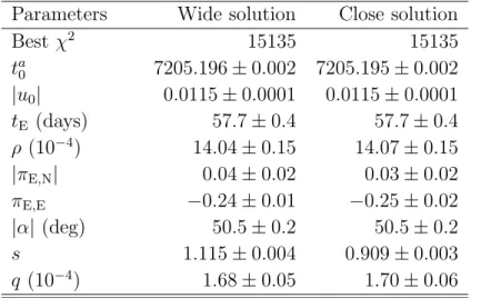
Within each set of solutions (wide or close) the physical implications are even closer, to the point of being nearly identical. Therefore, we present in Table 2 a simplified summary of each set of solutions, with the parameter values being averages over the four solutions
and the “errors” taking account of both the fit errors at different minima and the differences between minima.
4. Einstein Radius Estimate
We estimate θE using the standard approach (Yoo et al. 2004), i.e., estimating the source surface brightness from its dereddened color (V −I)0and the calibrated color/surface-brightness relation of Kervella et al. (2004), and then comparing this to dereddened magni-tude Is,0.
We begin (as is usual) by assuming that the source is behind the same dust column as the bulge clump stars. The field shows substantial differential reddening, so we restrict to a 60′′ radius about the source, wherein the clump appears compact. Using OGLE data, we find that the source lies ∆I = 3.15 mag below the clump, whereas using CTIO data we find ∆I = 3.01. This difference is typical of the difficulty in centroiding the clump in the vertical (magnitude) direction. We adopt ∆I = 3.08 ± 0.07 and so Is,0 = Icl,0+ ∆I = 17.54 where Icl,0 = 14.41 is adopted from Nataf et al. (2013).
Determining (V −I)s(and so (V −I)s,0) presents greater challenges given that the source is quite faint at baseline V ∼ 21.9 and that the full moon was passing through the bulge when the source was most highly magnified. OGLE systematically acquires V -band data for all its fields, but of course avoids observing near the Moon. Hence, the OGLE (V − I)0 color estimate has relatively large errors: ∆(V − I)s = −0.29 ± 0.06. CTIO deliberately targeted the event near peak (and so Moon passage) in order to obtain high signal-to-noise measurements. Some of these observations were corrupted by scattered moonlight, but most appear fine. These data yield ∆(V −I)s= −0.35±0.03. We combine these OGLE and CTIO measurements by standard error weighting and obtain (V − I)s,0 = (V − I)cl,0+ ∆(V − I) = 0.72 where we have adopted (V − I)cl,0 = 1.06 from Bensby et al. (2013). If we assume that the source is exactly at the distance to the clump and adopt MI,cl = −0.12, then this implies [MI, (V − I)0]s = (2.96, 0.72). This is a plausible pair of values for a star just entering the sub-giant branch from the turnoff. That is, the assumption that the source lies behind all the dust is self-consistent, since it implies that the source inhabits a reasonably well-populated part of the color-magnitude diagram.
However, another interpretation is that the source lies on the upper main sequence (since its color is similar to the Sun). Then, MI ∼ 4.15, so that the star lies 1.2 mag in front of the Bulge in distance modulus, or at DS ∼ 4.5 kpc from us. In this case, it would still lie about 125 pc below the Galactic plane and so behind most but possibly not all the dust toward the Galactic bulge.
subgiant and then address how this estimate may be affected if the source is in fact a disk main sequence star. After using Bessell & Brett (1988) to convert (V − I) to (I − K), the above procedure leads to estimates,
θ∗ = 1.07 ± 0.10 µas; θE= θ∗ ρ = 0.76 mas; µgeo = θE tE = 4.8 mas yr−1. (5) If the source were a disk main sequence star, but nevertheless lay behind all the dust, then these estimates would not be affected at all. Only the dereddened color and magnitude enter the calculation, and these would not change. If the source does lie in front of some of the dust, then it is both intrinsically redder in (V −I) and fainter in I than the above calculations would imply. Of course fainter stars have smaller radii at fixed surface brightness, but redder stars have lower surface brightness (so larger radii) at fixed magnitude. Hence, these two effects tend to cancel. Since the total amount of dust behind the source is unlikely to be large and the two effects tend to cancel, and since at this point we cannot reliably estimate how much dust does lie behind the source, we will proceed on the assumption that the source is behind all of the dust. However, in Section 6, we discuss how this issue could be partly or fully resolved in the future.
5. Physical Parameters
The extraction of physical parameters is made simpler by the “resolution” (or rather irrelevance) of the ambiguity of the amplitude of ∆β (Section 3), but more complicated by the ambiguity in the source distance (Section 4). We begin therefore with the lens mass estimate, which does not depend on the source distance
M = θE κπE
= 0.38 ± 0.04 M⊙; mplanet = qM = 21 ± 2M⊕ (6) Similarly, for the projected velocity in the geocentric and heliocentric frames
˜ vgeo(N, E) = AU tE πE π2 E = (0, −124)km s−1 v˜hel = ˜vgeo+ v⊕,⊥ = (0, −95)km s−1 (7) where v⊕,⊥(N, E) = (−0.8, 28.8)km s−1 is Earth’s velocity projected on the plane of the sky at the peak of the event and where we have ignored the slight differences among the four wide solutions.
Regardless of the source location, the relative parallax is well-determined
πrel = θEπE= 0.19 mas, (8)
but depending on the distance to the source, this leads to two different distance estimates for the lens DL = 3.3 kpc (bulge source) or DL = 2.5 kpc (disk source). However, within
the context of our program of determining the Galactic distribution of planets, these two outcomes are basically similar: foreground disk lens. In Section 6, we discuss how this ambiguity may be resolved with future observations.
Finally, the ambiguity in DL gives rise to an ambiguity of the same size in the star-planet projected separation r⊥ = sθEDL = 2.7 AU (bulge source) or 2.1 AU (disk source). Adopting a snowline rsnow = 2.7 AU (M/M⊙), these separations are at r⊥/rsnow = 2.2 and 1.7 snow-line distances, respectively. Hence, in either case, this planet is a “cold Neptune”. Note that in making these estimates, we have adopted s = 1, i.e., midway between (and 10% different from) the close and wide solutions.
6. Discussion
This is the second microlensing planet (after OGLE-2014-BLG-0124Lb), whose mass and distance have been characterized with the aid of parallax observations using Spitzer. However, it is the first to be so characterized as part of a program specifically designed to measure the Galactic distribution of planets by means of well-defined selection criteria (Yee et al. 2015a). While naively such well-defined criteria might seem to lead to clear cut observing decisions, the example of OGLE-2015-BLG-0966 demonstrates that they in fact create a set of complex interlocking constraints, both hard and soft, on decision processes of multiple semi-autonomous decision makers working toward a common goal. Specifically, there was the struggle to determine whether surveys would cover this event, including both static but non-obvious (KMT) information and dynamic OGLE information, impact on bal-ancing with coverage of other events (also impacted by survey coverage), and wild oscillations in Spitzer cadence due to objective criteria. See Section 2.
In the present case, these follow-up observations that were subject to these interlocking constraints led to detection and characterization of a planet while preserving the integrity of the selection process. In subsequent papers we will show that similar sensitivity to planets (while maintaining sample integrity) was achieved under similar conditions for several other high-magnification events.
The character of the planet, continues to confirm that “cool Neptunes are common” (Gould et al. 2006), even though that original claim was based on just two detections. How-ever, the central focus of the present effort is not the frequency of planets as a function of mass, but of Galactocentric radius. Nothing can be said so far about this in part because there are so far only two planets in the sample, but mainly because the sensitivity of the surveys to planets as a function of Galactocentric radius has not yet been determined (al-though see Zhu et al. 2015b for initial work in that direction). Nevertheless, it is intriguing to note that both detected planets are in the near-to-mid disk.
While the lens is clearly in the disk, it is unknown at this point whether the source is in the bulge or the disk. While the source distance is of overall secondary interest, it does affect the lens distance DL and planet-star separation r⊥ at the 25% level and therefore should be resolved if possible. We note that the heliocentric projected velocity ˜vhel does tend to favor a disk source just because the solutions all have the heliocentric projected velocities pointing basically out of the Galactic plane, and indeed somewhat retrograde. By contrast, as expected naively (and confirmed by Calchi Novati et al. 2015) events with bulge sources and disk lenses tend to have ˜vhel aligned with Galactic rotation. This is because the Sun and the lens both basically partake of this rotation while bulge source proper motions tend to be both isotropically distributed and of low amplitude.
The situation would be greatly clarified by measuring the proper motion of the source, as Yee et al. (2015b) did for the Spitzer event OGLE-2014-BLG-0939. In contrast to that case, however, in which the source was bright and easily distinguished from neighbors, which enabled precise astrometric measurements from over a decade of OGLE observations, the OGLE-2015-BLG-0966 source star is both too faint and too close (0.7′′) to a neighbor for re-liable astrometry. However, using difference image astrometry applied to high-magnification images, the current position of the lens is measured with a precision of about 20 mas. Hence, a single epoch of high-resolution imaging 10 years from now should be able to reliably de-termine whether the source proper motion is consistent with disk motion (typically about 6 mas yr−1).
This work is based in part on observations made with the Spitzer Space Telescope, which is operated by the Jet Propulsion Laboratory, California Institute of Technology under a contract with NASA.
The OGLE project has received funding from the National Science Centre, Poland, grant MAESTRO 2014/14/A/ST9/00121 to AU
Work by JCY, AG, and SC was supported by JPL grant 1500811. Work by JCY was performed under contract with the California Institute of Technology (Caltech)/Jet Propul-sion Laboratory (JPL) funded by NASA through the Sagan Fellowship Program executed by the NASA Exoplanet Science Institute
Work by C.H. was supported by Creative Research Initiative Program (2009-0081561) of National Research Foundation of Korea.
GD acknowledges Regione Campania for support from POR-FSE Campania 2014-2020. TS acknowledges the financial support from the JSPS, JSPS23103002,JSPS24253004 and JSPS26247023. The MOA project is supported by the grant JSPS25103508 and 23340064.
The US portion of the MOA Collaboration acknowledges financial support from the NSF (AST-1211875) and NASA (NNX12AF54G).
Work by YS was supported by an appointment to the NASA Postdoctoral Program at the Jet Propulsion Laboratory, administered by Oak Ridge Associated Universities through a contract with NASA.
This publication was made possible by NPRP grant # X-019-1-006 from the Qatar National Research Fund (a member of Qatar Foundation)
S.D. is supported by the Strategic Priority Research ProgramThe Emergence of Cos-mological Structures of the Chinese Academy of Sciences (grant No. XDB09000000).
Work by SM has been supported by the Strategic Priority Research Program “The Emergence of Cosmological Structures” of the Chi- nese Academy of Sciences Grant No. XDB09000000, and by the National Natural Science Foundation of China (NSFC) under grant numbers 11333003 and 11390372.
M.P.G.H. acknowledges support from the Villum Foundation. Based on data collected by MiNDSTEp with the Danish 1.54 m telescope at the ESO La Silla observatory. JSur-dej and OW acknowledge support from the Communaut franaise de Belgique Actions de recherche concertes Acadmie Wallonie-Europe. SHG and XBW would like to thank the financial support from National Natural Science Foundation of China through grants Nos. 10873031 and 11473066.
This work makes use of observations from the LCOGT network, which includes three SUPAscopes owned by the University of St Andrews. The RoboNet programme is an LCOGT Key Project using time allocations from the University of St Andrews, LCOGT and the University of Heidelberg together with time on the Liverpool Telescope through the Science and Technology Facilities Council (STFC), UK. This research has made use of the LCOGT Archive, which is operated by the California Institute of Technology, under contract with the Las Cumbres Observatory.
REFERENCES Alard, C. & Lupton, R.H., 1998, ApJ, 503, 325
Bachelet, ´E. et a., 2012, ApJ, 754, 73.
Bensby, T. Yee, J.C., Feltzing, S. et al. 2013, A&A, 549A, 147 Bessell, M.S., & Brett, J.M. 1988, PASP, 100, 1134
Bramich, D.M. 2008, MNRAS, 386, L77.
Bramich, D.M. et al, 2013, MNRAS, 428, 2275.
Brown, T.M., Baliber, N., Bianco, F.B. et al., 2013, PASP, 125, 1031 Calchi Novati, S., Gould, A., Udlaski, A., et al., 2015, ApJ, 804, 20 Cassan, A., Kubas, D., Beaulieu, J.-P., et al. 2012, Natur, 481, 167 Dominik, M. et al., 2008, AN, 329, 248.
Dominik, M. et al. 2010,AN, 331, 671.
Gaudi, B.S. & Gould, A. 1997, ApJ, 477, 152 Gould, A. 1994, ApJ, 421, L75
Gould, A. 1995, ApJ, 441, L21 Gould, A. 1996, ApJ, 470, 201
Gould, A, Udalski, A., An, D., et al. 2006, ApJ, 644, L37 Gould, A., Dong, S., Gaudi, B.S. et al. 2010, ApJ, 720, 1073 Gould, A. & Horne, K. 2013, ApJ, 779, 28
Gould, A., Carey, S., & Yee, J. Galactic Distribution of Planets from Spitzer Microlens Parallaxes Spitzer Proposal ID#11006
Griest, K. & Safizadeh, N. 1998, ApJ, 500, 37
Harpsøe, K. B. W., Jørgensen, U. G., Andersen, M. I., & Grundahl, F. 2012, A&A, 542, A23.
Horne, K., Tsapras, Y. & Snodgrass, C., 2009, MNRAS, 396, 2087. Hundertmark, M.P.G. et al., 2015, in prep.
Kervella, P., Th´evenin, F., Di Folco, E., & S´egransan, D. 2004, A&A, 426, 297 Nataf, D.M., Gould, A., Fouqu´e, P. et al. 2013, ApJ, 769, 88
Poindexter, S., Afonso, C., Bennett, D.P., Glicenstein, J.-F., Gould, A, Szyma´nski, M.K., & Udalski, A. 2005, ApJ, 633, 914
Refsdal, S. 1966, MNRAS, 134, 315
Schechter, P.L., Mateo, M., & Saha, A. 1993, PASP, 105, 1342
Skottfelt, J., Bramich, D.M., Hundertmark, M., et al. 2015, A&A, 574, A54 Shvartzvald et al. 2015, in prep.
Suzuki, D., Bennett, D.P., Sumi, T. et al. 2015, in prep
Udalski, A.,Szymanski, M., Kaluzny, J., Kubiak, M., Mateo, M., Krzeminski, W., & Paczy´nski, B. 1994, Acta Astron., 44, 317
Udalski, A. 2003, Acta Astron., 53, 291
Udalski, A., Yee, J.C., Gould, A., et al. 2015, ApJ, 799, 237
Udalski, A., Szyma´nski, M.K. & Szyma´nski, G. 2015, Acta Astronom., 65, 1
Yee, J.C., Gould, A., Beichman, C., et al. 2015a, ApJ, submitted, arXiv:1505.00014 Yee, J.C., Udalski, A., Calchi Novati, S., et al. 2015b, ApJ, 802, 76
Yoo, J., DePoy, D.L., Gal-Yam, A. et al. 2004, ApJ, 603, 139 Zhu, W., Udalski, A., Gould, A., et al. 2015a, ApJ, 805, 8
Zhu, W., Gould, A., Beichman, C., et al. 2015b, ApJ, submitted arXiv:1508.03336
–
24
–
Parameters (+, +),wide (+, −),wide (−, +),wide (−, −),wide (+, +),close (+, −),close (−, +),close (−, −),close χ2 /dof 15136/15278 15138/15278 15137/15278 15135/15278 15136/15278 15151/15278 15154/15278 15135/15278 t0 7205.1979 7205.1953 7205.1955 7205.1937 7205.1978 7205.1945 7205.1936 7205.1938 0.0012 0.0013 0.0013 0.0012 0.0012 0.0012 0.0012 0.0012 u0 0.01136 0.01136 -0.01157 -0.01152 0.01136 0.01136 -0.01162 -0.01149 0.00010 0.00010 0.00010 0.00010 0.00010 0.00010 0.00010 0.00009 tE (days) 57.7 57.8 57.7 57.7 57.7 57.7 57.5 57.8 0.4 0.4 0.4 0.4 0.4 0.5 0.4 0.4 ρ (10−4) 14.08 14.00 14.06 14.06 14.07 14.02 14.12 14.04 0.14 0.15 0.14 0.13 0.15 0.15 0.15 0.14 πE,N 0.0234 -0.0561 0.0397 -0.0412 0.0234 -0.0538 0.0317 -0.0412 0.0012 0.0015 0.0012 0.0013 0.0012 0.0059 0.0094 0.0012 πE,E -0.238 -0.237 -0.232 -0.237 -0.239 -0.264 -0.272 -0.237 0.006 0.012 0.003 0.006 0.006 0.007 0.007 0.006 α (deg) 50.7 50.6 -50.4 -50.4 50.6 50.6 -50.3 -50.4 0.1 0.1 0.1 0.1 0.1 0.1 0.1 0.1 s 1.1141 1.1146 1.1148 1.1147 0.9093 0.9091 0.9088 0.9091 0.0033 0.0032 0.0033 0.0033 0.0026 0.0025 0.0027 0.0026 q (10−4) 1.67 1.67 1.68 1.68 1.70 1.70 1.71 1.70 0.05 0.05 0.05 0.05 0.05 0.05 0.06 0.05 Blend -0.027 -0.024 -0.027 -0.026 -0.027 -0.025 -0.031 -0.024 0.008 0.009 0.008 0.008 0.008 0.008 0.008 0.008 Note. —aHJD-2450000.
7160
7180
7200
7220
7240
HJD-2450000
−0.4
−0.2
0.0
0.2
0.4
Re
sid
ua
l (m
ag
)
14.5
15.0
15.5
16.0
16.5
17.0
17.5
18.0
18.5
19.0
19.5
I (O
GL
E)
[m
ag
]
OGLE MOA Spitzer CTIO SMARTS LCOGT SSO LCOGT SAAO A LCOGT SAAO B LCOGT SAAO C LCOGT CTIO A LCOGT CTIO B LCOGT CTIO C Danish7205
7206
14.7
15.0
15.3
Fig. 1.— OGLE-2015-BLG-0966 lightcurve. Combined data from 10 telescopes (color coded) trace the ground-based light curve nearly continuously. With the exception of the ∼ 6 hr post peak bump, it is well characterized by a high-magnification point-lens Paczy´nski (1986) curve. As described in the text, five of the seven parameters (t0, u0, tE, α, ρ) needed to describe this curve can be read off lightcurve or extracted with very simple analysis. The remaining two (s, q) (planet-star separation and mass ratio) require more detailed modeling. The Spitzer lightcurve is aligned to the OGLE scale so that equal “magnitudes” represent equal magnifications. The microlens parallax πE can be well-estimated simply by comparing the Spitzer and ground-based light curves. See Section 3. (OGLE and MOA data are binned for display in the Figure, but not in the fit. Ground-based data points with uncertainties > 0.2 mag are suppressed in the figure to avoid clutter, but are included in the fit.)
0.2 0.1 0.0 -0.1 -0.2 θ/θE (East) -0.2 -0.1 0.0 0.1 θ/θ E ( No rt h) (+,−) −0.2 −0.1 0.0 0.1 0.2 θ/θ E ( No rt h) (+,+) 0.1 0.0 -0.1 -0.2 θ/θE (East) (−,+) Earth Spitzer (−,−) Close solutions 0.2 0.1 0.0 -0.1 -0.2 θ/θE (East) -0.2 -0.1 0.0 0.1 θ/θ E ( No rt h) (+,−) −0.2 −0.1 0.0 0.1 0.2 θ/θ E ( No rt h) (+,+) 0.1 0.0 -0.1 -0.2 θ/θE (East) (−,+) Earth Spitzer (−,−) Wide solutions
Fig. 2.— Thumb-nail sketches of all eight caustic geometries for planetary microlensing event OGLE-2015-BLG-0966. The black and red lines represent the trajectories as seen from Earth and Spitzer, respectively. The right ends of the red lines represent the end of Spitzer observations at HJD 7222.14. All eight solutions have essentially the same physical implications. First, while the overall caustic structures (closed black curves) differ between close (left) and wide (right) binary solutions, the central caustics, which are the only part probed by the Earth and Spitzer observations, are virtually identical. These are related by the s ↔ s−1 degeneracy, and since s ≃ 1.1 is close to unity, they correspond to physically similar systems. The microlens parallax πE is essentially determined by the offset between Spitzer and Earth trajectories at the same epoch (magenta dashed line segments). See Equation (3). The amplitude of πE does differ slightly between the (±, ±) and (±, ∓) solutions because the source is on the same side of the lens as seen from Earth and Spitzer for the former and on the opposite side for the latter, leading to a different distance perpendicular to the direction of motion. However, because the event is high magnification as seen from Earth (u0,⊕ ≪ 1), this difference is itself small, and because the separation along the direction of motion is much larger than the separation perpendicular, this has almost no effect on the magnitude of the parallax, πE, which is what enters the main physical parameters. See Table 1. The only substantial difference among these eight solutions is that the motion is somewhat north of west for the (+, ±) solutions and somewhat south of west for the (−, ±) solutions. However, this small difference has no impact on the main physical parameters, which do not depend on this direction.
0.02
0.01
0.00
-0.01
-0.02
θ/θ
E(East)
-0.02
-0.01
0.00
0.01
0.02
θ/θ
E(
N
or
th
)
OGLE
Spitzer
CTIO SMARTS
Danish
LCOGT SSO
LCOGT SAAO A
LCOGT SAAO B
LCOGT SAAO C
LCOGT CTIO A
LCOGT CTIO B
LCOGT CTIO C
MOA
Fig. 3.— Detail of caustic structure for one of the eight degenerate solutions shown in Figure 2 (close (−, −)). The colored circles represent the data points on the light curve shown in Figure 1. The black filled circle on the trajectory represents the size of the source. As described in Section 3, the angle between source trajectory and the binary axis (same as the caustic axis) is determined directly by the time offset of the anomalous peak from the overall peak, relative to the curvature of the peak, without reference to any model. However, the derivation of (s, q), which determines the overall caustic structure in this plot, does require detailed modeling. See Section 3.
Table 2: Abbreviated table of parameter values averaged over the four solutions. Parameters Wide solution Close solution
Best χ2 15135 15135 ta 0 7205.196 ± 0.002 7205.195 ± 0.002 |u0| 0.0115 ± 0.0001 0.0115 ± 0.0001 tE (days) 57.7 ± 0.4 57.7 ± 0.4 ρ (10−4) 14.04 ± 0.15 14.07 ± 0.15 |πE,N| 0.04 ± 0.02 0.03 ± 0.02 πE,E −0.24 ± 0.01 −0.25 ± 0.02 |α| (deg) 50.5 ± 0.2 50.5 ± 0.2 s 1.115 ± 0.004 0.909 ± 0.003 q (10−4) 1.68 ± 0.05 1.70 ± 0.06 aHJD-2450000