Early 2017 observations of TRAPPIST-1 with Spitzer
L. Delrez,
1
?
M. Gillon,
2
A. H. M. J. Triaud,
3
B.-O. Demory,
4
J. de Wit,
5
J. G. Ingalls,
6
E. Agol,
7,8
E. Bolmont,
9,10
A. Burdanov,
2
A. J. Burgasser,
11
S. J. Carey,
6
E. Jehin,
2
J. Leconte,
12
S. Lederer,
13
D. Queloz,
1
F. Selsis,
12
and V. Van Grootel
2
1 Cavendish Laboratory, JJ Thomson Avenue, Cambridge, CB3 0HE, UK
2 Space Sciences, Technologies and Astrophysics Research (STAR) Institute, Universit´e de Li`ege, All´ee du 6 Aoˆut 19C, B-4000 Li`ege, Belgium
3 School of Physics & Astronomy, University of Birmingham, Edgbaston, Birmingham B15 2TT, United Kingdom 4 University of Bern, Center for Space and Habitability, Gesellschaftsstrasse 6, CH-3012, Bern, Switzerland
5 Department of Earth, Atmospheric and Planetary Sciences, Massachusetts Institute of Technology, 77 Massachusetts Avenue, Cambridge, MA 02139, USA
6 IPAC, California Institute of Technology, 1200 E California Boulevard, Mail Code 314-6, Pasadena, California 91125, USA 7 Astronomy Department, University of Washington, Seattle, WA, 98195, USA; Guggenheim Fellow
8 NASA Astrobiology Institute’s Virtual Planetary Laboratory, Seattle, WA, 98195, USA 9 IRFU, CEA, Universit´e Paris-Saclay, F-91191 Gif-sur-Yvette, France
10Universit´e Paris Diderot, AIM, Sorbonne Paris Cit´e, CEA, CNRS, F-91191 Gif-sur-Yvette, France 11Center for Astrophysics and Space Science, University of California San Diego, La Jolla, CA, 92093, USA
12Laboratoire d’astrophysique de Bordeaux, Univ. Bordeaux, CNRS, B18N, All´ee Geoffroy Saint-Hilaire, F-33615 Pessac, France 13NASA Johnson Space Center, 2101 NASA Parkway, Houston, Texas, 77058, USA
Accepted 2017 December 31. Received 2017 December 21; in original form 2017 October 12
ABSTRACT
The recently detected TRAPPIST-1 planetary system, with its seven planets transit-ing a nearby ultracool dwarf star, offers the first opportunity to perform comparative exoplanetology of temperate Earth-sized worlds. To further advance our understand-ing of these planets’ compositions, energy budgets, and dynamics, we are carryunderstand-ing out an intensive photometric monitoring campaign of their transits with the Spitzer Space Telescope. In this context, we present 60 new transits of the TRAPPIST-1 planets observed with Spitzer /IRAC in February and March 2017. We combine these obser-vations with previously published Spitzer transit photometry and perform a global analysis of the resulting extensive dataset. This analysis refines the transit parame-ters and provides revised values for the planets’ physical parameparame-ters, notably their radii, using updated properties for the star. As part of our study, we also measure precise transit timings that will be used in a companion paper to refine the planets’ masses and compositions using the transit timing variations method. TRAPPIST-1 shows a very low level of low-frequency variability in the IRAC 4.5-µm band, with a photometric RMS of only 0.11% at a 123-s cadence. We do not detect any evidence of a (quasi-)periodic signal related to stellar rotation. We also analyze the transit light curves individually, to search for possible variations in the transit parameters of each planet due to stellar variability, and find that the Spitzer transits of the planets are mostly immune to the effects of stellar variations. These results are encouraging for forthcoming transmission spectroscopy observations of the TRAPPIST-1 planets with the James Webb Space Telescope.
Key words: planetary systems – stars: individual: TRAPPIST-1 – techniques: pho-tometric
c
2017 The Authors
1 INTRODUCTION
Small stars are beneficial for the discovery and study of
ex-oplanets by transit methods (e.g.Nutzman & Charbonneau
2008;He et al. 2017). For a given planet’s size and irradia-tion, they offer deeper planetary transits, and shorter orbital periods. The seven Earth-sized worlds orbiting the nearby
ultracool dwarf star TRAPPIST-1 (Gillon et al. 2016,2017,
hereafterG16andG17respectively) have become prime
tar-gets for the study of small planets beyond the Solar sys-tem, including the study of their atmospheres, owing to their transiting configuration combined with the infrared
bright-ness (K=10.3) and Jupiter-like size (∼0.12 R ) of their host
star (de Wit et al. 2016;Barstow & Irwin 2016;Morley et al. 2017).
The TRAPPIST-1 planets have further importance. There are approximately three times as many M-dwarfs as
FGK-dwarfs in the Milky Way (Kroupa 2001;Chabrier 2003;
Henry et al. 2006), and small planets appear to surround M-dwarfs three to five times more frequently than Sun-like stars (e.g.Bonfils et al. 2013;Dressing & Charbonneau 2013,
2015). If this trend continues to the bottom of the
main-sequence (see He et al. 2017), the TRAPPIST-1 planets
could well represent the most common Earth-sized planets in our Galaxy, which in itself would warrant special atten-tion. TRAPPIST-1 also presents an interesting numerical and dynamical challenge; for example, assessing its stability on Gyr timescales for orbital periods that have day to week timescales (Tamayo et al. 2016,2017).
A comparative study of the TRAPPIST-1 planets is aided by the fact that they all transit the same star. Be-cause the knowledge of most planetary parameters (e.g., mass and radius) is dependent on knowing these parameters for their parent stars, it is often difficult to make accurate comparisons across systems. Although the parameters of the TRAPPIST-1 planets remain dependent on the parameters of their host star, we can nevertheless compare the planets to one another. Furthermore, the planets have emerged from the same nebular environment, have experienced a similar history in terms of irradiation (notably in the XUV range; Wheatley et al. 2017;Bourrier et al. 2017;O’Malley-James & Kaltenegger 2017), and similar volatile delivery and at-mospheric sculpting via cometary impacts (Kral et al. sub-mitted). Thus, any differences among the planets must be the result of distinctions in their development. One example
would be the possible detection of O2, which on Earth has
biological origins but on other worlds can be produced abio-logically through the photodissociation of water vapour and
escape of hydrogen (e.g.Wordsworth & Pierrehumbert 2014;
Bolmont et al. 2017). The presence of significant O2on only
one of the seven planets would indicate a process particular to that planet, such as microbial respiration, with poten-tially far-reaching implications in humanity’s search for life beyond the Earth.
To improve the characterization of the planets in the TRAPPIST-1 system, and prepare for exploration of their atmospheric properties with the upcoming James Webb
Space Telescope (JWST) mission (Barstow & Irwin 2016;
Morley et al. 2017), we are conducting an intensive, high-precision, space-based photometric monitoring campaign of the system with Spitzer (Exploration Program ID 13067). The main goals of this program are to improve the
plan-ets’ transit parameters - notably to refine the determina-tion of their radii - and to use the measured transit tim-ing variations (TTVs) to constrain their masses and orbits (Agol et al. 2005;Holman & Murray 2005). Our Spitzer pro-gram also aims to study the infrared variability of the host star and its possible impact on the future JWST observa-tions, and to obtain first constraints on the presence of at-mospheres around the planets by comparing their transit depths measured in the infrared by Spitzer to the ones
mea-sured at shorter wavelengths by other facilities (e.g.de Wit
et al. 2016).
In this paper, we present observations gathered dur-ing the Feb-Mar 2017 window of visibility of the star by Spitzer. These new data more than double the number of transit events observed on TRAPPIST-1 with Spitzer.
Sec-tion2describes the data and data reduction. In Section3,
we combine these observations with previous Spitzer transit
photometry of TRAPPIST-1 presented inG17, and perform
a global analysis that enables us to significantly improve the planets’ transit parameters. We also use updated physical
parameters for the star (Van Grootel et al. 2017), to
re-vise the planets’ physical parameters, notably their radii. In addition, we assess the low-frequency infrared variability of the star and its impact on our measured quantities. As part of our analysis, we also extract precise transit timings. Our TTV analysis of the current timing dataset, including these new Spitzer timings, the resulting updated planetary masses, and our interpretations on the planets’ composition and formation, are presented in a separate companion
pa-per (Grimm et al. 2017). In Section 4, we discuss our
re-sults, examining variability in the transit parameters over the breadth of the dataset, and setting limits on wavelength-dependent transit depths for TRAPPIST-1b as a probe of its atmospheric properties. We summarize our results in Section5.
2 OBSERVATIONS AND DATA REDUCTION
As part of our Warm Spitzer Exploration Science program (ID 13067), Spitzer monitored 9, 16, 9, 6, 4, 3, and 1 new transit(s) of TRAPPIST-1b, -1c, -1d, -1e, -1f, -1g, and -1h, respectively, in the 4.5-µm channel of its Infrared Array
Camera (IRAC,Fazio et al. 2004). Twelve additional
tran-sits of TRAPPIST-1b were also observed with IRAC in the 3.6-µm channel. All these observations were performed be-tween 18 Feb and 27 Mar 2017. The corresponding data can
be accessed using the Spitzer Heritage Archive1(SHA). The
observations were obtained in subarray mode (32 × 32 pixels windowing of the detector) with an exposure time of 1.92 s. They were made without dithering (continuous staring) and in the pointing calibration and reference sensor (PCRS)
peak-up mode (Ingalls et al. 2012), which maximizes the
accuracy in the position of the target on the detector so as to minimize the so-called “pixel phase effect” of IRAC
in-dium antinomide arrays (e.g.Knutson et al. 2008). All the
data were calibrated with the Spitzer pipeline S19.2.0, and delivered as cubes of 64 subarray images of 32 × 32 pixels (pixel scale = 1.2 arcsec).
Our photometric extraction was identical to that
de-scribed inG17. After converting fluxes from MJy/sr to
pho-ton counts, we used the iraf/daophot2 software (Stetson
1987) to measure aperture photometry for the star within a
circular aperture of 2.3 pixels. The apertures for each image were centered on the stellar point-spread function (PSF) by fitting to a 2D-Gaussian profile, which also yielded measure-ments of the PSF width along the x and y image coordinates. Images with discrepant measurements for the PSF center, background flux, or source flux were discarded as described inGillon et al.(2014). We then combined the measurements per cube of 64 images. The photometric errors were taken as the errors on the average flux measurements for each cube.
We complemented the resulting set of light curves with
the Spitzer transit photometry previously published inG17,
consisting of 16, 11, 5, 2, 3, 2, and 1 transit(s) of TRAPPIST-1b, -1c, -1d, -1e, -1f, -1g, and -1h, respectively, all observed
with IRAC at 4.5µm. We refer the reader toG17and
ref-erences therein for more details about these data.
Our extensive Spitzer dataset thus includes a total of 37, 27, 14, 8, 7, 5, and 2 transits of planets b, c, d, e, f, g, and h, respectively. A few of these light curves showed flare signatures for which we discarded the corresponding measurements.
3 DATA ANALYSIS
Our data analysis was divided into three steps. We first per-formed individual analyses of the transit light curves
(Sec-tion3.1) to select the optimal photometric model for each
light curve, measure the transit timings, and assess the vari-ability of the transit parameters for each planet due to stel-lar variability. We then performed a global analysis of the
whole dataset (Section 3.2) with the aim of improving our
knowledge of the system parameters. Finally, we used our ex-tensive Spitzer dataset to assess the low-frequency infrared variability of the star in the IRAC 4.5-µm channel (Section 3.3).
Our individual and global data analyses were all carried out using the most recent version of the adaptive Markov
Chain Monte-Carlo (MCMC) code presented inGillon et al.
(2012, see also Gillon et al. 2014). We refer the reader to
these papers and references therein for a detailed descrip-tion of the MCMC algorithm and only describe below the aspects that are specific to the analyses presented here.
3.1 Individual analyses
We first converted each UT time of mid-exposure to the
BJDTDBtime-scale, as described byEastman et al.(2010).
We then performed an individual model selection for each light curve, using the transit model ofMandel & Agol(2002) multiplied by a photometric baseline model, different for each light curve, aiming to represent the other astrophys-ical and instrumental effects at the source of photometric
2 IRAF is distributed by the National Optical Astronomy Obser-vatory, which is operated by the Association of Universities for Research in Astronomy, Inc., under cooperative agreement with the National Science Foundation.
variations. A quadratic limb-darkening law was assumed for the star. For each light curve, we explored a large range of baseline models and selected the one that minimizes the
Bayesian Information Criterion (BIC,Schwarz 1978). This
led us to first include a linear or quadratic function of the x- and y-positions of the stellar PSF center (as measured in the images by fitting a two-dimensional Gaussian profile) in the baseline model of every light curve to account for the
pixel phase effect (e.g.Knutson et al. 2008). For some light
curves, the modeling of this effect was improved by comple-menting the x- and y-polynomial with a numerical position model computed with the bi-linearly-interpolated sub-pixel
sensitivity (BLISS) mapping method (Stevenson et al. 2012).
The sampling of the position space (number of grid points) was selected so that at least five measurements were located
in each sub-pixel box. We refer the reader toGillon et al.
(2014) for more details about the implementation of this
ap-proach in the MCMC code. We found that including a linear or quadratic function of the measured FWHM of the stellar PSF in the x- and/or y-directions resulted in a significant
decrease in the BIC for most light curves (similar to
Lan-otte et al. 2014and Demory et al. 2016). A polynomial of the logarithm of time was also required for some light curves to represent a sharp decrease of the detector response at the beginning of the observations (the so-called “ramp effect”, Knutson et al. 2008). Finally, a polynomial of time was also included in the baseline model for a fraction of the light curves to represent low-frequency signals likely related to
the rotational variability of the star (seeG16,Luger et al.
2017a, and Section3.3).
For each individual analysis, the jump parameters of the MCMC, i.e. the parameters randomly perturbed at each step of the Markov chains, were as follows:
• The stellar mass M?, radius R?, effective
tempera-ture Teff, and metallicity [Fe/H]. We assumed the normal
distributions N (0.0802,0.00732) M
, N (0.117,0.00362) R ,
N (2559,502) K, and N (0.04,0.082) dex as respective prior
probability distribution functions (PDFs) for these four
pa-rameters based on the values given inG17.
• For each transit (some light curves cover several
tran-sits), the transit depth dF = (Rp/R?)2 where Rp is the
ra-dius of the transiting planet, the transit impact parameter
b = acos i/R? where a is the orbital semi-major axis and
i is the orbital inclination, the transit width W (defined as the duration from first to last contact), and the time of mid-transit T0.
• The linear combinations of the quadratic
limb-darkening coefficients (u1, u2) in the considered bandpass,
c1= 2×u1+u2and c2= u1− 2 × u2. For each bandpass, values
and errors for u1and u2were interpolated for TRAPPIST-1
from the tables ofClaret & Bloemen(2011) and the
corre-sponding normal distributions were used as prior PDFs. For these individual analyses, we kept the orbital period(s)
of the relevant planet(s) fixed to the value(s) reported inG17
(for TRAPPIST-1b, c, d, e, f, g) andLuger et al.(2017a, for
TRAPPIST-1h). As inG17, we assumed circular orbits for
all the planets (eccentricity e= 0).
For each light curve, a preliminary MCMC analysis composed of one chain of 10 000 steps was first performed to estimate the correction factors CF to be applied to the pho-tometric error bars, to account for both the over- or
under-T1b [3.6 µm] 0.707 0.698 0.715 0.689 0.724 T1b [4.5 µm] 0.727 0.720 0.735 0.712 0.742 T1c [4.5 µm] 0.694 0.687 0.700 0.680 0.707 T1d [4.5 µm] 0.356 0.349 0.363 0.342 0.370 T1e [4.5 µm] 0.480 0.470 0.489 0.461 0.499 T1f [4.5 µm] 0.634 0.624 0.644 0.614 0.654 T1g [4.5 µm] 0.764 0.753 0.775 0.742 0.786 T1h [4.5 µm] 0.346 0.332 0.360 0.318 0.374 Epoch [arbitrary] Transit Depth [%]
.
.
.
.
T1b [3.6 µm] 36.1 36.0 36.3 35.9 36.4 T1b [4.5 µm] 36.1 36.0 36.3 35.9 36.4 T1c [4.5 µm] 42.3 42.1 42.4 42.0 42.0 T1d [4.5 µm] 49.3 49.0 49.7 48.6 50.1 T1e [4.5 µm] 55.9 55.5 56.3 55.1 56.7 T1f [4.5 µm] 63.1 62.7 63.5 62.4 63.8 T1g [4.5 µm] 68.5 68.1 68.9 67.7 69.2 T1h [4.5 µm] 76.9 75.9 77.8 75.0 78.8 Epoch [arbitrary]Transit Width [minute]
.
.
.
.
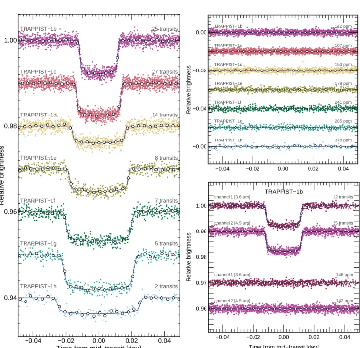
Figure 1. Left: Individual transit depth measurements for each of the events captured with Spitzer. The horizontal black line shows the median of the global MCMC posterior PDF (with its 1, and 2σ confidence, in shades of grey); the numeral values are also provided. Events are ranked in order of capture, left to right (but not linearly in time). Right: Similarly, but showing the duration of transit.
estimation of the white noise of each measurement and the
presence of correlated (red) noise in the data (see Gillon
et al. 2012 and Appendix B1 for details). Then, a longer MCMC analysis was performed, composed of two chains of 100 000 steps, whose convergence was checked using the sta-tistical test ofGelman & Rubin(1992).
Table A1 presents for each planet the transit timings,
depths, and durations deduced from the individual analyses of its transit light curves. For each planet, we performed a linear regression of the measured Spitzer transit timings as a function of their epochs to derive an updated mean transit
ephemeris (given in Table1). We show individual depths and
durations in Fig.1and see that in general, they are
compat-ible to one another, epoch after epoch, following close to a normal distribution. Our individual uncertainties on the du-ration appear all slightly over-estimated when we compare them to the mean of individual measurements. All planets
have reduced chi-squaredχ2r< 1 except for TRAPPIST-1b at
3.6µm, which has χ2r= 1.1. The situation is different for the
transit depths. TRAPPIST-1b (4.5 µm), -1c, -1d, -1f, and
-1h have χ2r compatible with normal distribution, whereas
TRAPPIST-1b (3.6 µm) has χ2
r = 4.4, TRAPPIST-1e has
χ2
r= 2.4, and TRAPPIST-1g has χ2r= 4.3. We discuss these
3.2 Global analysis
In a second phase, we carried out a global MCMC analysis of all the TRAPPIST-1 transits observed by Spitzer to im-prove the determination of the system parameters. We first performed a preliminary analysis, composed of one chain of 10 000 steps, to determine the correction factors CF to be applied to the error bars of each light curve (seeGillon et al.
2012and AppendixB1for details). With the corrected error
bars, we then performed the final global analysis, consisting of two Markov chains of 100 000 steps. The jump parameters in our global analysis were as follows:
• The stellar mass M?, radius R?, effective temperature
Teff, and metallicity [Fe/H].
• The linear combinations c1and c2of the quadratic
limb-darkening coefficients (u1, u2) for each bandpass, defined as
previously.
• For the seven planets, the transit depth dF4.5µm at
4.5µm, and the transit impact parameter b. The transit
du-ration was not a jump parameter anymore in the global anal-ysis, as it is uniquely defined for each planet by its orbital period, transit depth, and impact parameter, combined with the stellar mass and radius (Seager & Mall´en-Ornelas 2003). This assumption neglects orbital eccentricity and transit du-ration variations, which may be justified due to the small eccentricities expected when migrating into Laplace
reso-nances (Luger et al. 2017a), and the small amplitude of
tran-sit duration variations that is expected based on dynamical models.
• For TRAPPIST-1b, the transit depth difference
be-tween the Spitzer /IRAC 3.6-µm and 4.5-µm channels: ddF= dF3.6µm− dF4.5µm.
• For the six inner planets, the transit timing variation
(TTV) of each transit with respect to the mean transit ephemeris derived from the individual analyses (cf. Section 3.1).
• For TRAPPIST-1h, the orbital period P and the
mid-transit time T0.
This gives a total of 122 jump parameters for 19 258 data points. As previously, we assumed circular orbits for all the
planets. For M?, we used a normal prior PDF based on the
mass of 0.089 ± 0.007 M semi-empirically derived byVan
Grootel et al.(2017) for TRAPPIST-1 by combining a prior from stellar evolution models to a set of dynamical masses
recently reported by Dupuy & Liu (2017) for a sample of
equivalently classified ultracool dwarfs in astrometric bina-ries. We prefer here to assume this semi-empirical prior for the stellar mass rather than a purely theoretical one, like
the one used previously inG16andG17, as current stellar
evolutionary models are known to underestimate the radii of
some low-mass stars (e.g. Torres 2013,MacDonald &
Mul-lan 2014, and references therein; seeVan Grootel et al. 2017 for more details). We assumed the same normal prior PDFs
as previously for [Fe/H], and (u1, u2) for both bandpasses.
Uniform non-informative prior distributions were assumed for the other jump parameters.
The convergence of the chains was again checked with the statistical test ofGelman & Rubin(1992). The Gelman-Rubin statistic was less than 1.11 for every jump parameter, measured across the two chains, indicating that the chains are converged. We also estimated the effective sample size
Figure 2. Autocorrelation function for all 122 jump parameters versus chain lag,τ.
of the chains (Neff) by computing the integrated
autocorre-lation length as defined inGelman et al.(2013). We find a
minimum Neff of 27, with a median value of 118 over all
pa-rameters. Fig. 2shows the autocorrelation function versus
time lag for all 122 jump parameters.
The physical parameters of the system were deduced from the jump parameters at each step of the MCMC, so that their posterior PDFs could also be constructed. At
each MCMC step, the value for R? was combined with the
updated luminosity reported byVan Grootel et al.(2017),
L?= (5.22 ± 0.19) × 10−4 L , based on their improved
mea-surement of the star’s parallax, to derive a value for Teff. For
each planet, values for Rp, a, and i, were deduced from the
values for the stellar and transit parameters. Finally, val-ues were also computed for the irradiation of each planet in Earth units and for their equilibrium temperatures, assum-ing a null Bond albedo.
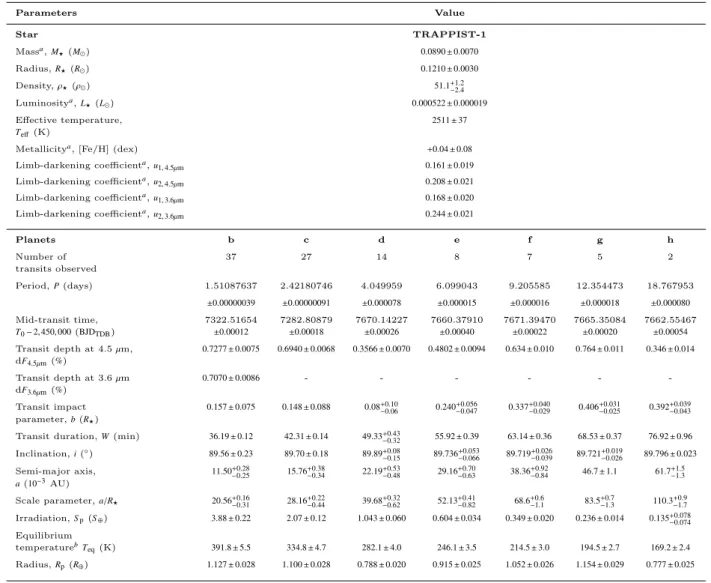
Fig.3 shows the detrended period-folded photometry
for each planet with the corresponding best-fit transit model,
while Figs.B1,B2, B3,B4, and B5display binned
residu-als RMS vs. bin size plots for the 78 light curves of our
dataset. Figs. B6 and B7 show the cross-correlation plots
and histograms of the posterior PDFs derived for the jump
parameters of our global analysis, while Table1presents the
parameters derived for the system. We discuss these results in Section4.
3.3 Stellar variability at 4.5µm
Monitoring the stellar variability with Spitzer is rendered difficult because of two factors. First, half of the Spitzer ob-servations analysed in this paper have been obtained in a time sparse mode, focusing on the transit windows of the seven TRAPPIST-1 planets. These sequences are short, up to four hours long, which is not enough to sample the rota-tional period of the star. Second, we failed to consistently position the target on the detector’s sweet spot, which sys-tematically affects the measured flux at the ∼2% level.
Fig-ure 4 illustrates the absolute flux level measured for all
TRAPPIST-1 AORs included in the present paper and the corresponding centroid locations on the detector. Two
dis-TRAPPIST−1b TRAPPIST−1c TRAPPIST−1d TRAPPIST−1e TRAPPIST−1f TRAPPIST−1g TRAPPIST−1h 25 transits 27 transits 14 transits 8 transits 7 transits 5 transits 2 transits −0.04 −0.02 0.00 0.02 0.04 0.94 0.96 0.98 1.00
Time from mid−transit [day]
Relative brightness
.
.
.
.
−0.04 −0.02 0.00 0.02 0.04 −0.06 −0.04 −0.02 0.00.
.
.
.
Relative brightness TRAPPIST−1b TRAPPIST−1c TRAPPIST−1d TRAPPIST−1e TRAPPIST−1f TRAPPIST−1g TRAPPIST−1h 142 ppm 107 ppm 150 ppm 179 ppm 241 ppm 285 ppm 378 ppm −0.04 −0.02 0.00 0.02 0.04 0.96 0.97 0.98 0.99 1.00.
.
.
.
TRAPPIST−1bTime from mid−transit [day]
Relative brightness channel 1 [3.6 µm] channel 2 [4.5 µm] 12 transits 25 transits channel 1 [3.6 µm] channel 2 [4.5 µm] 146 ppm 142 ppm
Figure 3. Left: Period-folded photometric measurements obtained by Spitzer at 4.5µm near the transits of planets TRAPPIST-1b to TRAPPIST-1h, corrected for the measured TTVs. Coloured dots show the unbinned measurements; open circles depict 5min-binned measurements for visual clarity. The best-fit transit models are shown as coloured lines. The number of transits that were observed to produce these combined curves is written on the plot. Top right: Corresponding residuals. The RMS of the residuals (5min bins) is indicated over each planet. Bottom right: Similar to other panels, only for TRAPPIST-1b at 3.6µm (channel 1) and 4.5 µm (channel 2).
tinct areas can be seen because of pointing inaccuracies due to the target’s large differential parallax between the Earth and Spitzer. To mitigate both caveats, we elect to conduct our variability analysis independently from the global fit presented above by only including the quasi-continuous
se-quence obtained over 21 days in Sept-Oct 2016 (G17). The
corresponding centroid locations are clustered on bottom right of Figure4.
We performed the data reduction by computing the ab-solute fluxes of all AORs using a fixed aperture size of 3
pixels throughout the dataset. A complication arose from the removal of the pixel-phase effect as TRAPPIST-1 fell 1 to 2 pixels away from the detector’s sweet spot for which a
high-resolution gain map exists (Ingalls et al. 2016). As no
such map was available for our purpose, we calibrated the absolute photometry by using the data itself, using an
im-plementation of the BLISS mapping algorithm (Stevenson
et al. 2012). We found that the entire area over which the star fell is relatively extended (0.6 pixels along the x-axis and 0.5 pixels along the y-axis), which marginally limits the flux
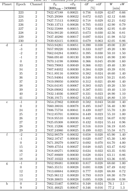
Table 1. Updated system parameters: median values and 1-σ limits of the posterior PDFs derived from our global MCMC analysis. Parameters Value Star TRAPPIST-1 Massa, M?(M ) 0.0890 ± 0.0070 Radius, R?(R ) 0.1210 ± 0.0030 Density,ρ?(ρ ) 51.1+1.2−2.4 Luminositya, L?(L ) 0.000522 ± 0.000019 Effective temperature, 2511 ± 37 Teff(K)
Metallicitya, [Fe/H] (dex) +0.04 ± 0.08
Limb-darkening coefficienta, u 1, 4.5µm 0.161 ± 0.019 Limb-darkening coefficienta, u 2, 4.5µm 0.208 ± 0.021 Limb-darkening coefficienta, u 1, 3.6µm 0.168 ± 0.020 Limb-darkening coefficienta, u 2, 3.6µm 0.244 ± 0.021 Planets b c d e f g h Number of 37 27 14 8 7 5 2 transits observed Period, P (days) 1.51087637 2.42180746 4.049959 6.099043 9.205585 12.354473 18.767953 ±0.00000039 ±0.00000091 ±0.000078 ±0.000015 ±0.000016 ±0.000018 ±0.000080 Mid-transit time, 7322.51654 7282.80879 7670.14227 7660.37910 7671.39470 7665.35084 7662.55467 T0− 2, 450, 000 (BJDTDB) ±0.00012 ±0.00018 ±0.00026 ±0.00040 ±0.00022 ±0.00020 ±0.00054 Transit depth at 4.5µm, 0.7277 ± 0.0075 0.6940 ± 0.0068 0.3566 ± 0.0070 0.4802 ± 0.0094 0.634 ± 0.010 0.764 ± 0.011 0.346 ± 0.014 dF4.5µm(%) Transit depth at 3.6µm 0.7070 ± 0.0086 - - - -dF3.6µm(%) Transit impact 0.157 ± 0.075 0.148 ± 0.088 0.08+0.10−0.06 0.240+0.056−0.047 0.337+0.040−0.029 0.406+0.031−0.025 0.392+0.039−0.043 parameter, b (R?)
Transit duration, W (min) 36.19 ± 0.12 42.31 ± 0.14 49.33+0.43−0.32 55.92 ± 0.39 63.14 ± 0.36 68.53 ± 0.37 76.92 ± 0.96 Inclination, i (◦)
89.56 ± 0.23 89.70 ± 0.18 89.89+0.08−0.15 89.736+0.053−0.066 89.719+0.026−0.039 89.721+0.019−0.026 89.796 ± 0.023 Semi-major axis, 11.50+0.28−0.25 15.76+0.38−0.34 22.19+0.53−0.48 29.16+0.70−0.63 38.36+0.92−0.84 46.7 ± 1.1 61.7+1.5−1.3 a (10−3AU)
Scale parameter, a/R? 20.56+0.16−0.31 28.16+0.22−0.44 39.68+0.32−0.62 52.13+0.41−0.82 68.6+0.6−1.1 83.5+0.7−1.3 110.3+0.9−1.7 Irradiation, Sp(S⊕) 3.88 ± 0.22 2.07 ± 0.12 1.043 ± 0.060 0.604 ± 0.034 0.349 ± 0.020 0.236 ± 0.014 0.135+0.078−0.074 Equilibrium
temperaturebT
eq(K) 391.8 ± 5.5 334.8 ± 4.7 282.1 ± 4.0 246.1 ± 3.5 214.5 ± 3.0 194.5 ± 2.7 169.2 ± 2.4
Radius, Rp(R⊕) 1.127 ± 0.028 1.100 ± 0.028 0.788 ± 0.020 0.915 ± 0.025 1.052 ± 0.026 1.154 ± 0.029 0.777 ± 0.025
Notes.a Informative prior PDFs were assumed for these stellar parameters (see Section3.2). bAssuming a null Bond albedo.
calibration accuracy. For the purposes of this stellar vari-ability analysis, we discarded flares and removed transits based on the parameters deduced from our global analysis
(Table1). The photometric residuals are thus assumed to
in-clude signal from the star alone. We measured a photometric residual RMS of 0.11% at a 123-s cadence. We performed a discrete Fourier analysis of the residuals that yielded a max-imum at ∼10 days. The 3.30 ± 0.14-day rotation period found byLuger et al.(2017a, see alsoVida et al. 2017) using 80-day continuous observations of visible K2 data, appears as a low-amplitude peak in our periodogram.
To obtain a more detailed view of the signal compo-nents, we further perform a wavelet analysis of the pho-tometric residuals. For this purpose, we use the weighted
wavelet Z-transform (WWZ) code presented in Foster
(1996). The wavelet Z-statistic is computed as a function
of both time and frequency, which gives further insights into the structure of the photometric residuals. The results of
this analysis are shown on Figure5. We find that multiple
peaks exist but that are of low amplitude. No signal is ap-parent around 3.3 days but the ∼10-day signature seems to
persist across the entire window, albeit of low significance. The low-amplitude residual correlated noise could originate from imperfect instrumental systematic correction or from stellar noise. Assuming that the systematics correction we use is efficient, the wavelet analysis applied to the photomet-ric residuals suggests that the star exhibits multiple active regions that evolve rapidly with time. The data at hand does not enable us to clearly identify the structure of the signal. We argue that long-term parallel monitoring of TRAPPIST-1 in the visible and infrared are desirable to better constrain its variability patterns.
We carried out an additional analysis of the power spec-trum of TRAPPIST-1 using a correlated noise model scribed by a Gaussian process with a power spectrum de-fined as the sum of stochastically-driven damped simple-harmonic oscillators, each with quality factor Q and
fre-quency ω0 (Foreman-Mackey et al. 2017). We fit the data
with two components: a fixed Q= 1/√2 term which has a
power spectrum describing variability similar to granulation, and a second Q>> 1 term describing (quasi-)periodic vari-ability, with a frequency initialized for a period of 3 days.
14.5 15.0 15.5 16.0 16.5 14.0 14.5 15.0 15.5 16.0 14.5 15.0 15.5 16.0 16.5 x 14.0 14.5 15.0 15.5 16.0 y 2.80•104 2.85•104 2.90•104 2.95•104
Measured Flux (e-/frame)
Figure 4. TRAPPIST-1 Spitzer /IRAC raw photometric fluxes collected from all 66 AORs taken between 2016 and March 2017 and the corresponding centroid locations on the detector.
0.2 0.4 0.6 0.8 1.0 Frequency (cycles/day) 0 50 100 150 200 250 Relative Z statistic 7655 7660 7665 7670 BJD_TDB 1.004 1.002 1.000 0.998 0.996 Relative flux
Figure 5. Wavelet diagram (top) of the photometric residuals (bottom).
We found that the amplitude of the large-Q term decreased to zero when optimizing the parameters of the Gaussian pro-cess, indicating that there is no evidence for quasi-periodic variability in the Spitzer 4.5-µm dataset. We found that the “granulation” term had a finite amplitude with a variance of 7 × 10⁻⁴, and a frequencyω0= 22.45 rad day−1, corresponding
to a characteristic damping timescale of 0.28 days. Once the power spectrum was optimized, we subtracted off the Gaus-sian process estimate of the correlated noise component, and found that the normalized residuals follow a Gaussian, but slightly broader by a factor of 1.065, which is an additional argument for increasing the uncertainties on the data points with the correction factors, CF, as discussed above.
4 DISCUSSION
4.1 Updated system parameters
We have more than doubled the number of transit events ob-served with Spitzer on TRAPPIST-1 with respect to what
has been presented inG17. Our global analysis refines the
planets’ transit depths (at 4.5 µm) by factors up to 2.8
(TRAPPIST-1e) and their transit durations by factors up to 2.8 (TRAPPIST-1h), and also slightly improves the pre-cision of the physical parameters derived for the planets.
An important point to outline is that inG16and G17our
global analysis assumed an informative prior on the stellar mass and radius - and thus on the stellar density - based on stellar evolution models. In this new analysis, no informative prior was assumed for the stellar radius, and the stellar den-sity was only constrained by the shape of the transits of the seven planets (Seager & Mall´en-Ornelas 2003). Furthermore, our assumed prior on the stellar mass was here not only based on stellar physics computations but also on empirical
data (see Section3.2andVan Grootel et al. 2017). We thus
consider our updated planetary parameters presented in
Ta-ble1not only more precise than those reported inG17, but
also more accurate because they are less model-dependent. We compare some of these quantities to Solar system objects
and the rest of the small exoplanet population in Fig.6.
4.2 Variability of the transit parameters
As reported in Section 3.3, we do not find any significant
(quasi-)periodic signal in the IRAC 4.5-µm band related to the rotation of TRAPPIST-1. Rotational variability has
however been previously detected by Luger et al. (2017a)
in the K2 passband, at the level of few percents and with a period of ∼3.3 days. This periodic photometric variability indicates that inhomogeneities of the stellar surface (spots)
move in and out of view as the star rotates. Luger et al.
(2017b) recently demonstrated that the orbital planes of
the TRAPPIST-1 planets are aligned to<0.3◦ at 90%
con-fidence. Together, the planets cover at least 56% of a
hemi-sphere when they transit (shadowed area in Fig.7), notably
the low and intermediate latitudes at which we find spots
on the Sun (e.g.Miletskii & Ivanov 2009). We could
there-fore expect the planets to cross some stellar spots during their transits. Such occulted spots would affect the transit profile in a way that would depend on their size, contrast, and distribution across the planetary chord, and would tend to make the transit shallower. Unocculted spots, i.e., stellar spots that are not crossed during planetary transits, would have the opposite effect, making the transit deeper by dimin-ishing the overall flux from the star while leaving the sur-face brightness along the transit chord unchanged. Because of stellar spots, either occulted or unocculted, we could thus expect to detect variations in the planets’ transit depths as a function of time.
As noted in Section3.1, the transit depths derived from
the individual analyses generally follow a normal
distri-bution for each planet, except TRAPPIST-1b at 3.6 µm,
TRAPPIST-1e, and TRAPPIST-1g, each of which show some outliers. It is common knowledge that transit param-eters derived from a single transit light curve can be
1b 1c 1d 1e 1f 1g 1h 0.1 1.0 0.2 2. 0.5 5. 0.7 0.8 0.9 1.0 1.1 1.2 1.3
.
.
.
.
Incident flux [Searth]Planetary radius [R
earth
]
Earth
Venus
Mercury Mars Ceres
TRAPPIST−1 system 0.1 1.0 10.0 100.0 1000. 0.1 1.0 0.2 0.5 Earth Mercury Mars Venus Ceres K2−9 b EPIC 206318379 b GJ1132 b LHS1140 b GJ1214 b Kepler−42 d, c & b solar−like red dwarfs brown dwarfs TRAPPIST−1 h, g, f, e, d, c & b
.
.
.
.
Incident flux [Searth]Stellar mass [M
sol
]
Figure 6. Updates on diagrams shown inG16andG17. Left: Planetary radii as a function of incident flux. Right: Planet population shown ordered by stellar-host mass as a function of incident flux. Only planets with radii< 2R⊕are represented. The dots size increases linearly with radius.
global analysis of an extensive set of transit light curves, which assumes one unique transit profile for all the transit light curves (of a same planet), allows a better separation of the actual transit signal from the correlated noise and the derivation of robust transit parameters. To better assess the possible variations in the transit depth of each planet, we computed for each of its transits the median values of the photometric residuals in transit and out of transit, using for this purpose the photometric residuals from the global analysis. These median values, together with the median
ab-solute deviations, are given for each transit in Table B1.
A significant difference between the in-transit and out-of-transit medians of the photometric residuals for a given tran-sit would indicate a variation in its depth compared to the planet’s transit depth derived from the global analysis. How-ever, the in-transit and out-of-transit medians are compati-ble within 1 sigma for all transits of all planets. This test re-veals that the variability seen for some planets
(TRAPPIST-1b at 3.6 µm, TRAPPIST-1e, and TRAPPIST-1g) in the
transit depths derived from the individual analyses is likely not physical but rather caused by systematic effects –which are better disentangled from the planetary signals in the global analysis.
In this context, it is worth noting that instrumental
systematics are stronger at 3.6µm than at 4.5 µm and thus
require more complex baseline models, which can introduce some biases in the transit parameters derived from a sin-gle light curve. This might explain the increased scatter of
TRAPPIST-1b’s individual transit depths at 3.6 µm. For
TRAPPIST-1e, we note that only the first transit in Fig.1
(epoch -1) shows a discrepant transit depth. This transit was actually observed over two different consecutive AORs, which might have introduced a bias in its measured depth.
As for TRAPPIST-1g, a visual inspection of the global anal-ysis’ residuals for the two transits with discrepant transit
depths (second and fifth transits in Fig.1, corresponding to
epochs 0 and 14 respectively) does not reveal any obvious structures or spot-crossings. The origin of these two outliers thus remains unclear. Additional transit observations of this planet at higher SNR are needed to better assess the possi-ble variability of its transit depth.
Overall, Spitzer transits of TRAPPIST-1 planets thus appear to be mostly immune to the effects of stellar vari-ability. There are several reasons why this may happen:
• Considering the very low level of low-frequency
photo-metric variability shown by TRAPPIST-1 at 4.5µm,
unoc-culted spots may not have a significant impact on the
plan-ets’ transit depths. Using the simple model of Berta et al.
(2011, see their Equations 8 and 9) to estimate the expected
amplitude of transit depth variations at 4.5µm due to
unoc-culted spots based on the stellar variability measured in that band, we indeed find amplitudes lower than 100 ppm for all the planets. This is smaller than the error bars on the indi-vidual transit depths. We note however that this estimate is only a lower limit to the possible amplitude of transit depth variations due to unocculted spots. Indeed, the rotational variability of the star reflects only the non-axisymmetric component of the stellar surface inhomogeneities. The ax-isymmetric component does not contribute to the measured stellar variability and its effect is thus not included in our es-timate, while it is also expected to affect the planets’ transit depths.
• The periodic variability detected in the K2 passband
may be caused by high-latitude spots that do not cross the planets’ chords, explaining the non-detection of spot-crossing events. Evidence for such high-latitude spots has
1g 1h 1f 1e 1b 1c 1d −1.0 −0.5 0.0 0.5 1.0 −1.0 −0.5 0.0 0.5 1.0
.
.
.
.
Stellar radius (Rs)Figure 7. Representation of the star, and of the planets that transit it, using impact parameters and transit depths from Ta-ble 1. The planets cover a minimum area of ∼56% of an hemi-sphere. Planetary position on its chord is arbitrary.
been reported for some mid- and late-M dwarfs (see e.g. Barnes et al. 2015). We note however that these objects are usually young (.1 Gyr), while TRAPPIST-1 is a rather old
system (7.6 ± 2.2 Gyr,Burgasser & Mamajek 2017).
• Spot-crossing events may not produce detectable effects
on the Spitzer transit light curves due to the reduced spot-to-photosphere contrast in the IRAC passbands (see e.g. Ballerini et al. 2012). A practical example of this effect was
presented byFraine et al.(2014), who reported simultaneous
Kepler and Spitzer transit photometry of the Neptune-sized planet HAT-P-11b orbiting an active K4 dwarf. While some spot-crossing events are clearly visible in the Kepler optical photometry, they are undetected in the photometry obtained
concurrently with Spitzer at 4.5µm.
4.3 Transmission spectrum of TRAPPIST-1b
A transmission spectrum can be severely affected by both oc-culted and unococ-culted stellar spots (e.g.Jord´an et al. 2013; McCullough et al. 2014;Rackham et al. 2017). To extract a proper transmission spectrum, a planet needs to cover a part of the stellar surface that has a spectrum that is representa-tive of the whole disc. We are in a privileged position with TRAPPIST-1 as the planets cross over a quarter of the entire stellar surface, and more than half of a hemisphere. Unless spots never intersect transit chords, the planets will cross over a representative fraction of the star, and the transmis-sion spectra measured for the TRAPPIST-1 planets should
be robust measures of their atmospheres (de Wit et al. 2016;
Barstow & Irwin 2016;Morley et al. 2017).
Our global data analysis yields a marginal transit depth
difference of +208 ± 110 ppm for TRAPPIST-1b between
the Spitzer /IRAC 4.5-µm and 3.6-µm channels, the
tran-sit being slightly deeper at 4.5 µm than at 3.6 µm
(Ta-ble1). If confirmed, this transit depth variation would
im-ply that TRAPPIST-1b’s atmosphere significantly exceeds its equilibrium temperature (392 K assuming a null Bond
albedo, Table 1). A deeper transit depth at 4.5µm would
be best explained by atmospheric CO2, which has a
promi-nent absorption feature around 4.2µm (see e.g.,
Kalteneg-ger & Traub 2009). The most favorable scenario to en-hance such a signature requires no other opacity source across the IRAC 3.6-µm channel than the extended wing
of the 4.2-µm absorption band of CO2. In such a case, the
variation in transit depth is approximately equivalent to 5 scale heights (H) at medium spectral resolution (see e.g., Kaltenegger & Traub 2009;de Wit & Seager 2013) and 2H when binned over IRAC’s channels. TRAPPIST-1b’s scale height would thus be larger or equal to approximately 52 km (208 ppm = ((Rp+2H)/R?)2− (Rp/R?)2). For comparison,
the Earth’s atmospheric scale height is 8.5 km, while that
of Venus is 15.9 km3. This lower limit on the planet
atmo-spheric scale height can be translated into a lower limit on its atmospheric temperature owing to assumptions of its
at-mospheric mean molecular mass,µ, and surface gravity, g.
Planet b’s surface gravity is approximately 8 m/s2 (Grimm
et al. 2017). Under the present assumption that no strong absorber affects the 3.6-µm band, the background gas can-not be water or methane–both exhibit absorption features in this band–implying that the atmosphere must have a large
µ (e.g., 28 u.m.a. if dominated by N2). Under such a
favor-able scenario for the CO2 feature, TRAPPIST-1 b’s
atmo-sphere would require an average temperature above 1400 K– more than three times larger than its estimated equilibrium temperature. On the other hand, if water dominates its at-mosphere, this would lead to two counter-balancing effects: (1) a decrease of the mean molecular weight and (2) a tran-sit depth variation between the two IRAC channels of no
more than a scale height due to water absorption at 3.3µm.
This would yield an atmospheric scale height larger than ∼100 km and an average atmospheric temperature above ∼1800 K. Other opacity sources, such as clouds or hazes, would require an even larger scale height and atmospheric temperature to support such a variation in transit depth be-tween the two IRAC channels. Therefore, if confirmed, such hint of variability would be indicative of a surprisingly large atmospheric temperature for TRAPPIST-1b.
As demonstrated recently by Deming & Sheppard
(2017), transit measurements of a planet transiting an
M-dwarf can be affected by a resolution-linked bias (RLB) ef-fect, which acts to decrease the apparent amplitude of an absorption feature from the planetary atmosphere. This is due to the complex line structure exhibited by M-dwarfs which creates a flux-leakage effect at low to medium spectral resolution wherein the stellar flux does not entirely cancel out in the ratio of in- to out-of-transit flux. We estimated the amplitude of the RLB effect on the transit depth dif-ference expected for TRAPPIST-1b between the IRAC 4.5-µm and 3.6-4.5-µm channels assuming different atmospheric
sce-narios, namely H2-, H2O-, N2-, and CO2-rich atmospheres
(de Wit et al. 2016). For TRAPPIST-1 spectrum, we used
the PHOENIX/BT-Settl model with Teff/log g/[M/H] of
2500K/5.5/0.0 (Allard et al. 2012). We find a maximal RLB effect of ∼115 ppm over a ∼2400 ppm absorption feature of
methane in a H2-rich atmosphere, which corresponds to a
dampening of the methane absorption feature by ∼5%. Al-though the amplitude of the effect in this case is comparable to the uncertainty on our measured transit depth difference, it is not relevant for the interpretation of our measurements as the hint of feature detected between the two IRAC chan-nels is not of the order of ∼2400 ppm. We find amplitudes ranging from only a few ppm to 30 ppm for the other atmo-spheric scenarios. The marginal difference in transit depth that we measure between both IRAC bands is thus not ex-pected to be significantly affected by the RLB effect.
5 CONCLUSIONS
In this work, we presented 60 new transits of the TRAPPIST-1 planets observed with Spitzer /IRAC in early 2017. We performed a global analysis of the entire Spitzer dataset gathered so far, which enabled us to refine the tran-sit parameters and to provide revised values for the plan-ets’ physical parameters, notably their radii, using updated properties for the host star. As part of this study, we also ex-tracted precise transit timings that will be instrumental for TTV studies of the system, to be presented in a companion paper. In addition, we found that the star shows a very low level of low-frequency variability in the IRAC 4.5-µm chan-nel. We did not detect any evidence of a (quasi-)periodic signal related to stellar rotation and found that the planets’ transit depths measured with Spitzer are mostly not affected by stellar variability. Finally, we also found for
TRAPPIST-1b a marginal transit depth difference of+208±110 ppm
be-tween the IRAC 4.5-µm and 3.6-µm channels. If confirmed, this transit depth variation could indicate the presence of
CO2in the planet’s atmosphere as well as a surprisingly large
atmospheric temperature. Together, these results improve our understanding of this remarkable system and help pre-pare the detailed atmospheric characterization of its planets with JWST.
ACKNOWLEDGEMENTS
We thank E. Gillen for interesting discussions and valu-able suggestions. This work is based in part on observations made with the Spitzer Space Telescope, which is operated by the Jet Propulsion Laboratory, California Institute of Technology, under a contract with NASA. This work was partially supported by a grant from the Simons Foundation (PI Queloz, grant number 327127). The research leading to these results also received funding from the European Re-search Council (ERC) under the FP/2007-2013 ERC grant agreement no. 336480, and under the H2020 ERC grant agreement no. 679030; and from an Action de Recherche
Concert´ee (ARC) grant, financed by the Wallonia-Brussels
Federation. L.D. acknowledges support from the Gruber Foundation Fellowship. V.V.G. and M.G. are F.R.S.-FNRS Research Associates. E.J. is F.R.S.-FNRS Senior Research Associate. B.-O.D. acknowledges support from the Swiss National Science Foundation in the form of a SNSF Pro-fessorship (PP00P2 163967). E.B. acknowledges funding by
the European Research Council through ERC grant SPIRE 647383. A.J.B. acknowledges funding support from the US-UK Fulbright Scholarship program.
REFERENCES
Agol E., Steffen J., Sari R., Clarkson W., 2005,MNRAS,359, 567 Allard F., Homeier D., Freytag B., 2012,Philosophical
Transac-tions of the Royal Society of London Series A,370, 2765 Ballerini P., Micela G., Lanza A. F., Pagano I., 2012,A&A,539,
A140
Barnes J. R., Jeffers S. V., Jones H. R. A., Pavlenko Y. V., Jenkins J. S., Haswell C. A., Lohr M. E., 2015,ApJ,812, 42 Barstow J. K., Irwin P. G. J., 2016,MNRAS,461, L92
Berta Z. K., Charbonneau D., Bean J., Irwin J., Burke C. J., D´esert J.-M., Nutzman P., Falco E. E., 2011,ApJ,736, 12 Bolmont E., Selsis F., Owen J. E., Ribas I., Raymond S. N.,
Leconte J., Gillon M., 2017,MNRAS,464, 3728 Bonfils X., et al., 2013,A&A,549, A109
Bourrier V., et al., 2017,A&A,599, L3
Burgasser A. J., Mamajek E. E., 2017,ApJ,845, 110 Chabrier G., 2003,PASP,115, 763
Claret A., Bloemen S., 2011,A&A,529, A75
Cubillos P., Harrington J., Loredo T. J., Lust N. B., Blecic J., Stemm M., 2017,AJ,153, 3
Deming D., Sheppard K., 2017,ApJ,841, L3
Demory B.-O., Gillon M., Madhusudhan N., Queloz D., 2016, MNRAS,455, 2018
Dressing C. D., Charbonneau D., 2013,ApJ,767, 95 Dressing C. D., Charbonneau D., 2015,ApJ,807, 45 Dupuy T. J., Liu M. C., 2017,ApJS,231, 15
Eastman J., Siverd R., Gaudi B. S., 2010,PASP,122, 935 Fazio G. G., et al., 2004,ApJS,154, 10
Foreman-Mackey D., 2016,The Journal of Open Source Software, 24
Foreman-Mackey D., Agol E., Ambikasaran S., Angus R., 2017, AJ,154, 220
Foster G., 1996,AJ,112, 1709 Fraine J., et al., 2014,Nature,513, 526
Gelman A., Rubin D. B., 1992,Statistical Science,7, 457 Gelman A., Carlin J., Stern H., Dunson D., Vehtari A., Rubin
D., 2013, Bayesian Data Analysis, Third Edition. Chapman & Hall/CRC Texts in Statistical Science, Taylor & Francis, https://books.google.fr/books?id=ZXL6AQAAQBAJ
Gillon M., et al., 2012,A&A,542, A4 Gillon M., et al., 2014,A&A,563, A21 Gillon M., et al., 2016,Nature,533, 221 Gillon M., et al., 2017,Nature,542, 456 Grimm S., et al., 2017, submitted to A&A
He M. Y., Triaud A. H. M. J., Gillon M., 2017,MNRAS,464, 2687
Henry T. J., Jao W.-C., Subasavage J. P., Beaulieu T. D., Ianna P. A., Costa E., M´endez R. A., 2006,AJ,132, 2360
Holman M. J., Murray N. W., 2005,Science,307, 1288
Ingalls J. G., Krick J. E., Carey S. J., Laine S., Surace J. A., Glac-cum W. J., Grillmair C. C., Lowrance P. J., 2012, in Space Telescopes and Instrumentation 2012: Optical, Infrared, and Millimeter Wave. p. 84421Y,doi:10.1117/12.926947
Ingalls J. G., et al., 2016,AJ,152, 44 Jord´an A., et al., 2013,ApJ,778, 184
Kaltenegger L., Traub W. A., 2009,ApJ,698, 519
Knutson H. A., Charbonneau D., Allen L. E., Burrows A., Megeath S. T., 2008,ApJ,673, 526
Kroupa P., 2001,MNRAS,322, 231 Lanotte A. A., et al., 2014,A&A,572, A73
Luger R., Lustig-Yaeger J., Agol E., 2017b, preprint, (arXiv:1711.05739)
MacDonald J., Mullan D. J., 2014,ApJ,787, 70 Mandel K., Agol E., 2002,ApJ,580, L171
McCullough P. R., Crouzet N., Deming D., Madhusudhan N., 2014,ApJ,791, 55
Miletskii E. V., Ivanov V. G., 2009,Astronomy Reports,53, 857 Morley C. V., Kreidberg L., Rustamkulov Z., Robinson T.,
Fort-ney J. J., 2017, preprint, (arXiv:1708.04239) Nutzman P., Charbonneau D., 2008,PASP,120, 317
O’Malley-James J. T., Kaltenegger L., 2017,MNRAS,469, L26 Rackham B., et al., 2017,ApJ,834, 151
Schwarz G., 1978, Annals of Statistics,6, 461 Seager S., Mall´en-Ornelas G., 2003,ApJ,585, 1038 Stetson P. B., 1987,PASP,99, 191
Stevenson K. B., et al., 2012,ApJ,754, 136 Tamayo D., et al., 2016,ApJ,832, L22
Tamayo D., Rein H., Petrovich C., Murray N., 2017, ApJ,840, L19
Torres G., 2013,Astronomische Nachrichten,334, 4 Van Grootel V., et al., 2017, preprint, (arXiv:1712.01911) Vida K., K˝ov´ari Z., P´al A., Ol´ah K., Kriskovics L., 2017,ApJ,
841, 124
Wheatley P. J., Louden T., Bourrier V., Ehrenreich D., Gillon M., 2017,MNRAS,465, L74
Winn J. N., et al., 2008,ApJ,683, 1076
Wordsworth R., Pierrehumbert R., 2014,ApJ,785, L20 de Wit J., Seager S., 2013,Science,342, 1473
de Wit J., et al., 2016,Nature,537, 69
APPENDIX A: RESULTS FROM THE INDIVIDUAL ANALYSES
Table A1: Median values and 1-σ limits of the posterior PDFs deduced for the timings, depths, and durations of the transits from their individual analyses.
Planet Epoch Channel T0 eT0 dF edF W eW
[BJDTDB− 2450000] [%] [min] b 78 2 7440.36514 0.00035 0.742 0.048 36.30 1.20 86 2 7452.45228 0.00014 0.757 0.025 35.76 0.40 93 2 7463.02847 0.00019 0.682 0.025 36.68 0.59 218 2 7651.88743 0.00022 0.774 0.040 36.36 0.69 219 2 7653.39809 0.00026 0.684 0.031 36.19 0.68 220 2 7654.90908 0.00084 0.759 0.024 35.80 2.20 222 2 7657.93129 0.00020 0.735 0.030 36.26 0.54 223 2 7659.44144 0.00017 0.746 0.029 36.84 0.58 224 2 7660.95205 0.00033 0.675 0.041 37.07 0.95 225 2 7662.46358 0.00020 0.757 0.036 36.39 0.60 226 2 7663.97492 0.00070 0.776 0.045 35.90 1.90 227 2 7665.48509 0.00017 0.772 0.032 36.45 0.50 228 2 7666.99567 0.00025 0.704 0.043 36.10 0.81 229 2 7668.50668 0.00030 0.728 0.041 36.54 0.81 230 2 7670.01766 0.00034 0.751 0.048 36.75 0.89 231 2 7671.52876 0.00030 0.702 0.045 36.78 0.86 318 2 7802.97557 0.00016 0.751 0.027 35.73 0.65 320 2 7805.99697 0.00016 0.699 0.023 36.29 0.50 321 2 7807.50731 0.00017 0.703 0.026 36.75 0.52 322 1 7809.01822 0.00017 0.801 0.028 36.01 0.65 324 2 7812.04038 0.00020 0.703 0.027 36.64 0.59 325 2 7813.55121 0.00014 0.732 0.022 36.43 0.43 326 1 7815.06275 0.00017 0.724 0.023 36.76 0.53 327 1 7816.57335 0.00011 0.663 0.021 35.36 0.35 328 2 7818.08382 0.00015 0.723 0.026 36.41 0.46 329 1 7819.59478 0.00017 0.704 0.028 36.21 0.53 330 1 7821.10550 0.00020 0.737 0.032 36.33 0.60 332 2 7824.12730 0.00018 0.737 0.029 36.29 0.55 333 1 7825.63813 0.00018 0.706 0.033 36.19 0.60 334 1 7827.14995 0.00012 0.742 0.023 36.33 0.42 335 1 7828.66042 0.00024 0.727 0.031 35.70 0.69 336 2 7830.17087 0.00021 0.708 0.032 36.44 0.60 338 1 7833.19257 0.00018 0.618 0.023 35.67 0.55 339 1 7834.70398 0.00016 0.682 0.020 37.14 0.49 340 2 7836.21440 0.00017 0.706 0.028 35.59 0.50 341 1 7837.72526 0.00014 0.702 0.023 35.74 0.56 342 1 7839.23669 0.00017 0.808 0.025 35.76 0.56 c 70 2 7452.33470 0.00015 0.698 0.023 42.28 0.48 71 2 7454.75672 0.00066 0.644 0.037 42.60 2.00 152 2 7650.92395 0.00023 0.708 0.029 43.59 0.79 153 2 7653.34553 0.00024 0.668 0.026 42.62 0.69 154 2 7655.76785 0.00040 0.679 0.050 43.10 1.00 155 2 7658.18963 0.00024 0.668 0.030 42.11 0.66 156 2 7660.61168 0.00051 0.681 0.056 42.20 1.30 157 2 7663.03292 0.00028 0.710 0.031 42.46 0.88 158 2 7665.45519 0.00025 0.719 0.030 42.18 0.65 159 2 7667.87729 0.00031 0.700 0.038 42.54 0.81 160 2 7670.29869 0.00035 0.731 0.044 42.34 0.96 215 2 7803.49747 0.00020 0.672 0.025 41.42 0.59 216 2 7805.91882 0.00017 0.652 0.020 42.21 0.48 217 2 7808.34123 0.00023 0.735 0.035 41.98 0.71 218 2 7810.76273 0.00019 0.674 0.029 42.45 0.62 219 2 7813.18456 0.00024 0.668 0.024 42.02 0.72 220 2 7815.60583 0.00017 0.725 0.024 42.88 0.55 221 2 7818.02821 0.00020 0.763 0.024 42.28 0.53 222 2 7820.45019 0.00022 0.674 0.024 41.76 0.60
Table A1 – continued from previous page
Planet Epoch Channel T0 eT0 dF edF W eW
[BJDTDB− 2450000] [%] [min] 223 2 7822.87188 0.00021 0.756 0.028 42.67 0.66 224 2 7825.29388 0.00022 0.672 0.025 42.12 0.66 225 2 7827.71513 0.00022 0.718 0.029 42.21 0.62 226 2 7830.13713 0.00026 0.705 0.033 42.90 0.79 227 2 7832.55888 0.00015 0.732 0.026 42.95 0.49 228 2 7834.98120 0.00025 0.673 0.030 42.56 0.81 229 2 7837.40280 0.00017 0.697 0.024 41.98 0.52 230 2 7839.82415 0.00031 0.679 0.063 42.05 0.86 d -4 2 7653.94261 0.00051 0.390 0.038 49.00 2.20 -3 2 7657.99220 0.00063 0.333 0.027 49.20 1.90 -2 2 7662.04284 0.00051 0.395 0.030 50.10 1.50 -1 2 7666.09140 0.00130 0.308 0.043 48.90 2.80 0 2 7670.14198 0.00066 0.366 0.045 49.00 1.60 33 2 7803.79083 0.00049 0.366 0.021 49.40 1.30 34 2 7807.84032 0.00030 0.384 0.020 49.39 0.91 35 2 7811.89116 0.00050 0.382 0.024 48.60 1.40 36 2 7815.94064 0.00030 0.348 0.019 50.21 0.85 37 2 7819.99050 0.00050 0.312 0.021 49.80 1.40 38 2 7824.04185 0.00067 0.383 0.025 49.20 1.50 39 2 7828.09082 0.00043 0.387 0.031 49.40 1.10 40 2 7832.14036 0.00037 0.331 0.023 48.90 1.10 41 2 7836.19171 0.00042 0.345 0.023 48.80 1.10 e -1 2 7654.27862 0.00049 0.582 0.043 58.60 1.40 0 2 7660.38016 0.00078 0.495 0.047 56.40 1.90 24 2 7806.75758 0.00041 0.439 0.027 55.70 1.20 25 2 7812.85701 0.00034 0.449 0.023 55.10 1.00 26 2 7818.95510 0.00030 0.482 0.022 56.07 0.92 27 2 7825.05308 0.00035 0.432 0.024 55.44 0.96 28 2 7831.15206 0.00027 0.516 0.018 56.19 0.85 29 2 7837.24980 0.00025 0.499 0.021 55.58 0.71 f -2 2 7652.98579 0.00032 0.658 0.020 65.90 1.40 -1 2 7662.18747 0.00040 0.620 0.037 65.30 1.80 0 2 7671.39279 0.00072 0.692 0.070 64.70 4.00 15 2 7809.47554 0.00027 0.648 0.025 63.47 0.82 16 2 7818.68271 0.00032 0.634 0.022 63.35 0.93 17 2 7827.88669 0.00030 0.628 0.024 63.11 0.86 18 2 7837.10322 0.00032 0.610 0.023 63.36 0.95 g -1 2 7652.99481 0.00030 0.817 0.028 68.60 1.00 0 2 7665.35151 0.00028 0.691 0.026 67.49 0.82 12 2 7813.60684 0.00023 0.777 0.020 68.88 0.72 13 2 7825.96112 0.00020 0.793 0.019 68.30 0.79 14 2 7838.30655 0.00028 0.695 0.026 68.08 0.98 h 0 2 7662.55467 0.00054 0.348 0.024 76.1 2.1 9 2 7831.46625 0.00047 0.346 0.016 77.2 1.3
APPENDIX B: GLOBAL ANALYSIS: SUPPLEMENTARY MATERIAL
B1 Binned residuals RMS vs. bin size plots
Figs.B1,B2,B3,B4, andB5show the RMS vs. bin size plots for the 78 Spitzer /IRAC light curves of our dataset, made
us-ing the binrms routine of the MC3open-source Python
pack-age (Cubillos et al. 2017). For each light curve, the RMS
of the binned residuals, RMSN, is shown as a black curve
for bin sizes (i.e. the mean number N of points in each bin) ranging from one to half the data size. The uncertainty of
RMSN(grey error bars) is computed asσRMS= RMSN/
√ 2M (seeCubillos et al. 2017for the derivation), where M is the
number of bins. The red curve shows the expected RMSσN
in the absence of correlated noise, given by (Winn et al.
2008): σN = σ1 √ N r M M −1 (B1)
where σ1 is the RMS of the unbinned residuals. The
saw-tooth look of this red curve arises from the discreet change in M, which becomes more significant as N increases.
As mentioned in Section3, the possible presence of
cor-related noise in the data is accounted for in our analyses via correction factors CF that we applied to the photomet-ric error bars of each light curve before performing the final analyses. For each light curve, CF is the product of two con-tributions,βwandβr. On one side,βwrepresents the
under-or overestimation of the white noise of each measurement. It is computed as the ratio between the RMS of the unbinned residuals and the mean photometric error. On the other side,
βr allows to account for possible correlated noise present in
the light curve, and is calculated as:
βr = RMSN σN (B2) = σN σ1 r N(M − 1) M (B3)
The largest value obtained with different bin sizes is kept as βr.
Figure B1. Binned residuals RMS (black curves with grey error bars) vs. bin size for the first eighteen Spitzer /IRAC light curves. The red curves are the expected RMS for Gaussian noise.
Figure B5. Same as Fig.B1, but for light curves 73 to 78.
B2 Cross-correlation plots of the posterior PDFs
Fig.B6shows the cross-correlation of the posterior
param-eters for the star from the global analysis made using
cor-ner.py (Foreman-Mackey 2016). Since the transit
duration-period relation constrains the density of the star strongly, the mass and radius are strongly correlated. As the luminos-ity prior is strongly constrained, the uncertainty in radius is anti-correlated with the effective temperature. The metal-licity correlates weakly with the other stellar parameters.
Fig.B7shows the correlations between transit impact
parameter and depth. As a common density for the star was used for all the transits, the impact parameters are strongly correlated as they anti-correlate with the transit durations, while the durations are well constrained by the data, and as zero eccentricity was assumed for the planet orbits. The depths correlate with the impact parameters as larger impact parameters have transit chords with lower sur-face brightness (due to limb-darkening), requiring a larger planet to cause the same transit depth.
The limb-darkening parameters and transit times cor-relate weakly with all of the other parameters, so we have not included these in the cross-correlation plots.
Figure B6. Cross-correlation plots and histograms of the pos-terior PDFs deduced for the stellar parameters from our global analysis.
Figure B7. Cross-correlation plots and histograms of the posterior PDFs of the transit depths and impact parameters for the seven planets, as well as the difference in transit depth of planet TRAPPIST-1b between IRAC channel 1 and channel 2.
B3 Median values of the residuals in and out of transit
Table B1: Median values (medianin, medianout) and median absolute deviations (σin and σout) of the residuals in and out of
transit, using the residuals from the global analysis. The last column gives the significance of the difference between medianin
and medianout, computed as |medianqin−medianout| σ2
in+σ 2 out
.
Planet Epoch medianin σin medianout σout Significance of
[ppm] [ppm] [ppm] [ppm] the difference [σ] b (3.6µm) 322 -188 421 213 600 0.55 326 -371 415 33 488 0.63 327 449 287 26 620 0.62 330 -9 350 -107 522 0.16 333 -107 522 151 588 0.33 334 -27 587 143 350 0.25 335 158 530 90 416 0.10 338 445 637 162 761 0.29 339 82 340 -153 334 0.49 341 295 293 -45 421 0.66 342 -407 635 219 579 0.73 b (4.5µm) 78 133 420 -290 464 0.68 86 -32 344 362 390 0.76 93 -240 303 -192 740 0.06 218 -265 407 350 588 0.86 219 279 527 -318 413 0.89 220 -386 353 194 550 0.89 222 -406 583 90 570 0.61 224 104 519 -240 659 0.41 225 -328 471 179 612 0.65 226 -136 372 196 480 0.55 227 -512 354 -361 621 0.21 228 192 279 -188 423 0.75 229 -226 831 -296 338 0.08 230 -242 732 -684 624 0.46 231 89 979 122 384 0.03 318 -59 382 -430 606 0.52 320 182 379 -67 473 0.41 321 -229 466 -27 669 0.25 324 226 417 14 561 0.30 325 208 553 199 538 0.01 328 -145 700 110 530 0.29 332 -45 530 -259 617 0.26 336 334 669 -41 1003 0.31 340 359 770 368 362 0.01 c 70 126 475 11 618 0.15 71 242 302 -171 404 0.82 152 -331 251 -645 360 0.71 153 102 405 -85 701 0.23 154 512 538 75 964 0.40 155 345 623 -11 658 0.39 156 -92 684 53 596 0.16 157 -167 742 -400 794 0.21 158 -89 371 -311 750 0.27 159 201 653 -168 391 0.48 160 -112 380 -113 780 0.00 215 124 602 -264 379 0.55 216 340 664 -165 676 0.53 217 -233 536 259 779 0.52 218 13 547 -82 612 0.12 219 83 721 -79 452 0.19 220 -32 472 96 670 0.16
Table B1 – continued from previous page
Planet Epoch medianin σin medianout σout Significance of
[ppm] [ppm] [ppm] [ppm] the difference [σ] 221 -208 711 18 398 0.28 222 333 501 -126 576 0.60 223 -241 509 286 614 0.66 224 90 772 -43 560 0.14 225 -229 561 -79 376 0.22 226 -71 602 -179 588 0.13 227 -93 556 -297 734 0.22 228 345 777 -98 333 0.52 229 14 507 -128 466 0.21 230 399 746 -115 559 0.55 d -4 -159 754 260 733 0.40 -3 110 472 112 551 0.00 -2 -59 849 -103 674 0.04 -1 61 593 -5 409 0.09 0 -83 538 -96 669 0.02 33 45 580 -63 721 0.12 34 -73 511 180 579 0.33 35 -87 723 23 451 0.13 36 157 428 185 478 0.04 37 313 652 -118 478 0.04 38 -18 727 189 656 0.21 39 -131 320 292 425 0.80 40 312 720 206 573 0.12 41 54 617 191 646 0.15 e -1 -128 627 159 763 0.29 0 -316 487 87 540 0.55 24 218 500 -257 446 0.71 25 -257 446 -49 693 0.25 26 -149 637 234 559 0.45 27 234 606 -392 508 0.79 28 -201 695 334 580 0.59 29 -251 531 -5 736 0.27 f -2 -235 635 27 512 0.32 -1 195 440 31 560 0.23 0 40 632 159 726 0.12 15 -205 516 -307 793 0.11 16 -274 641 188 493 0.57 17 -117 571 -203 612 0.10 18 79 621 -196 541 0.33 g -1 -235 635 -230 525 0.01 0 555 531 377 557 0.23 12 -48 336 +199 735 0.31 13 -165 611 209 334 0.54 14 143 609 -365 501 0.64 h 0 14 459 -26 646 0.05 9 -27 540 -155 557 0.16
This paper has been typeset from a TEX/LATEX file prepared by the author.