Preliminary JIRAM results from Juno polar observations: 3.
Evidence of diffuse methane presence in the Jupiter
auroral regions
M. L. Moriconi1,2 , A. Adriani1 , B. M. Dinelli1,2 , F. Fabiano2,3 , F. Altieri1 , F. Tosi1 , G. Filacchione1 , A. Migliorini1 , J. C. Gérard4 , A. Mura1 , D. Grassi1 , G. Sindoni1 , G. Piccioni1 , R. Noschese1, A. Cicchetti1 , S. J. Bolton5 , J. E. P. Connerney6 , S. K. Atreya7, F. Bagenal8 , G. R. Gladstone5 , C. Hansen9 , W. S. Kurth10 , S. M. Levin11 , B. H. Mauk12 , D. J. McComas13 , D. Turrini1,14 , S. Stefani1 , A. Olivieri15, and M. Amoroso15
1
INAF-Istituto di Astrofisica e Planetologia Spaziali, Rome, Italy,2CNR-Istituto di Scienze dell’Atmosfera e del Clima, Bologna, Italy,3Dipartimento di Fisica e Astronomia, Università di Bologna, Bologna, Italy,4Laboratoire de Physique Atmosphérique et Planétaire, Université de Liège, Liège, Belgium,5Space Science and Engineering Division, Southwest Research Institute, San Antonio, Texas, USA,6NASA Goddard Space Flight Center, Greenbelt, Maryland, USA,7Planetary Science Laboratory, University of Michigan, Ann Arbor, Michigan, USA,8Laboratory for Atmospheric and Space Physics, University of Colorado Boulder, Boulder, Colorado, USA,9Planetary Science Institute, Tucson, Arizona, USA,10Jet Propulsion Laboratory, California Institute of Technology, Pasadena, California, USA,11Department of Physics and Astronomy, University of Iowa, Iowa City, Iowa, USA,12The Johns Hopkins University Applied Physics Laboratory, Laurel, Maryland, USA,13Plasma Physics Laboratory, Princeton University, Princeton, New Jersey, USA,14Departamento de Fisica, Universidad de Atacama, Copiapò, Chile, 15Agenzia Spaziale Italiana, Rome, Italy
Abstract
Throughout thefirst orbit of the NASA Juno mission around Jupiter, the Jupiter InfraRed Auroral Mapper (JIRAM) targeted the northern and southern polar regions several times. The analyses of the acquired images and spectra confirmed a significant presence of methane (CH4) near both poles through its 3.3μmemission overlapping the H3+auroral feature at 3.31μm. Neither acetylene (C2H2) nor ethane (C2H6) have
been observed so far. The analysis method, developed for the retrieval of H3+temperature and abundances
and applied to the JIRAM-measured spectra, has enabled an estimate of the effective temperature for methane peak emission and the distribution of its spectral contribution in the polar regions. The enhanced methane inside the auroral oval regions in the two hemispheres at different longitude suggests an excitation mechanism driven by energized particle precipitation from the magnetosphere.
1. Introduction
The 3.3μm CH4emission from both the Jupiter polar regions has been detected in the past two decades
principally by Earth-based observations, with high spectral resolution but low spatial coverage depending from the relative positions of Jupiter and Earth at the time of those measurements [Kim et al., 1991, 2015; Caldwell et al., 1983]. More information on the horizontal distribution and temperatures of the emitting mole-cules has been obtained mainly for the northern polar region, easier to target than the southern one for its favorable orientation, but some hydrocarbon emissions near the south pole have been measured too [Caldwell et al., 1988; Kim et al., 2009, 2015]. Space-based measurements of hydrocarbon polar emissions have been performed by Galileo/Near-Infrared Mapping Spectrometer (NIMS) and Cassini/Composite Infrared Spectrometer [Sada et al., 2003]. The latter, however, probed the atmosphere at wavelengths longer than 3μm, sounding therefore different altitudes, temperatures, and probably emission mechanisms. In a recent study of some unexploited Galileo/NIMS data sets, Altieri et al. [2016] provided a map of the 3 μm CH4and
C2H2 emitting regions on the Jupiter north pole at high spatial resolution. Only one NIMS observation,
characterized by a nighttime coverage and a very slant viewing perspective, could be used to map the horizontal distribution of methane emitting molecules. This viewing geometry, quite similar to the ground-based ones, enabled a satisfactorily match with previousfindings reported in literature [Kim et al., 2015]. In this paper, we report the preliminary results obtained by the analysis of Jupiter InfraRed Auroral Mapper (JIRAM) observations during thefirst Juno orbit. We describe evidence of a diffuse 3.3 μm methane emission on both polar regions. The viewing geometries of the instrument during the perijove observations encom-passed several degrees of slant to nadir perspectives. In section 2 a short description of the instrument
Geophysical Research Letters
RESEARCH LETTER
10.1002/2017GL073592
Special Section:
Early Results: Juno at Jupiter
Key Points:
• Evidence of diffuse CH4emission
inside the northern and southern Jupiter auroral ovals
• Detailed maps of the distribution of the CH4emission are obtained for
both poles
• Estimated rotational temperatures of the CH4emission are about 500 K for
the north pole and 650 K for the south pole
Correspondence to:
M. L. Moriconi, m.moriconi@isac.cnr.it
Citation:
Moriconi, M. L., et al. (2017), Preliminary JIRAM results from Juno polar observa-tions: 3. Evidence of diffuse methane presence in the Jupiter auroral regions, Geophys. Res. Lett., 44, 4641–4648, doi:10.1002/2017GL073592.
Received 1 FEB 2017 Accepted 13 APR 2017 Published online 25 MAY 2017
©2017. American Geophysical Union. All Rights Reserved.
along with the data management and image processing techniques applied to detect the CH4fluorescence
[Drossart et al., 1999] from the observations is given. In section 3 some preliminary conclusions on CH4
tem-perature and distribution in the auroral regions are drawn, and in section 4 the principal outcomes of this work are summarized.
2. JIRAM Instrument and Data Management
JIRAM combines an imager and a spectrometer in one instrument. The two units share a common telescope [Adriani et al., 2014]. The experiment is completed by a despinning flat mirror, compensating for the Juno 2 rpm spin motion, and an internal calibration unit. The IR imager in turn splits into two spectral channels: the L band, centered at 3.45μm with a 290 nm bandwidth, and the M band, centered at 4.78 μm with a 480 nm bandwidth. Each imager has a 5.94° × 1.76°field of view (FOV) with an instantaneous field of view (IFOV) of 250 × 250μrad (128 × 432 pixel format). The spectrometer’s slit, colocated inside the M imager FOV, has a FOV of 3.52° sampled by 256 spatial samples in the wavelength range 2–5 μm (336 bands) with an average spectral sampling of ~9 nm/band and an approximate resolution of ~12 nm. The slit is combined with line 153 of the imager covering the pixels ranging from 88 to 343. Both imager and spectrometer mea-surements are geometrically calibrated by ad hoc algorithms based on the NAIF-SPICE tools [Acton, 1996]. The imager and spectrometer raw data are calibrated in radiance, according to Adriani et al. [2014]. During thefirst Juno orbit, JIRAM acquired 28 and 14 images in the L band, together with an equal number of spec-tral measurements covering the north and south aurorae, respectively. Specspec-tral slit measurements acquired in the same timeframe have been subsequently combined to obtain a series of hyperspectral images (here-after spectral frame) organized in cube data sets. Since the spectrometer acquires only one slit per Juno spacecraft rotation (e.g., one every 30 s), the footprints of the slit are not contiguous on the surface and need to be independently geolocated and reprojected to build an image [Adriani et al., 2016].
The spatial distribution and temperature of the 3.3μm CH4emission have been derived from the spectral
data, while the L band images have been used to verify and provide the global context and location of the emitting molecules [see Adriani et al., 2017, Figure 1].
Actually, the coverage obtained by the spectrometer does not extend over the whole imager FOV, and some-time the image reconstruction gives results below the expectation because of the large angular separation between consecutive scanning acquisitions.
The 3.3μm CH4emission spreads on a spectral region covered by three JIRAM channels centered at 3.315,
3.324, and 3.333μm. Hereafter we will refer to the 3.315 μm JIRAM channel, including most of the lines of the Q branches of the fundamental v3and the weaker v3+ v4-v4and v3+ v2-v2methane bands. However,
as some H3+emission lines are present in the same spectral region, a preliminary analysis with color
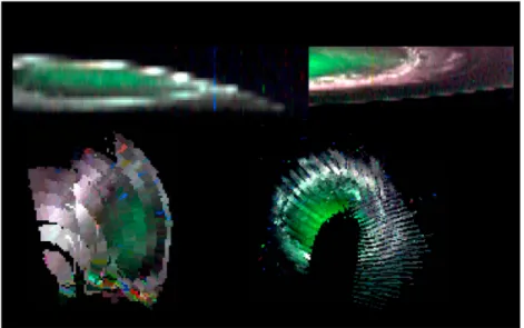
compo-site images has been performed to investigate the presence of methanefluorescence and its potential distri-bution in the Jupiter polar regions. In Figure 1 the north and south poles are both imaged as spectral frames, reconstructed by a single session of spectrometric measurements, and as a mosaic in stereographic projec-tion of some observaprojec-tion sessions targeting the poles. The wavelength color composiprojec-tion—red for 3.540μm, green for 3.315 μm, and blue for 3.423 μm—corresponds to the JIRAM channel where methane emission is present and to two other channels where only H3+auroral peaks are present. The wavelengths
have been chosen in a spectral region where scattering and thermal radiation are minimal.
Since the CH4 Q branch shares with the H3+ auroral emission the JIRAM channel at 3.315 μm, in the
presence of methanefluorescence and faint H3+emission the methane signal can prevail on the auroral
pattern. In the four panels shown in Figure 2 the selected wavelengths render the auroral emission in white color, as, in that case, the three H3+peak intensities are comparable and the CH4emission is absent or negligible. An overriding green region, or a predominance of the 3.315 μm component, identifies instead the presence of a diffuse methane fluorescence inside the auroral oval that prevails over the H3+ emission, regardless of the emission mechanism acting [Kim et al., 2015]. The north pole has been
observed in slant and in nadir observing geometries. In both cases the quality of the relative color com-posite spectral frames was lower than for the south pole images. Indeed, the northern slant observations have been acquired from a longer distance than the southern ones, with only a few scanning slits quite distant from each other. These observing conditions resulted in a lower spatial resolution and a blurry
reconstructed image due to the stressed interpolation between consecutive slits. North pole nadir observations have been acquired from a relatively short distance but have been therefore more contaminated by the environmental radiation. Nevertheless, the images of the northern polar region also clearly indicate the presence of CH4. In fact, as described in Dinelli et al. [2017], the inclusion of the CH4in the calculations is necessary to obtain reasonable H3+temperatures in the region where the
green color suggests the presence of methane in the observed spectra.
Figure 2. Summary of the outcomes from the correlation method applied to the 3.315μm and 3.540 μm spectral intensi-ties for the (a–d) north and (e–h) south JIRAM data sets. The scatterplots show two correlation sets, highlighted by green and red ellipses (Figures 2a and 2e). The spatial average calculated on the spectral pixels, relative to the points inside those ellipses, is reported in corresponding colors in Figures 2b and 2f, and the spatial distribution of those same pixels is shown in identical colors at the bottom of thefigure. The maps in Figures 2c, 2d, 2g, and 2h are in planetocentric System III coordinates.
Figure 1. (left column) Northern and (right column) southern aurorae pictured as a color composition of the wavelengths 3.540μm (red), 3.315 μm (green), and 3.423 μm (blue). (top row) The spectral frames acquired on 26 (north) and 27 (south) August 2016 are shown. (bottom row) The spectral frames, geolocated and projected as stereographic polar image, are composed of mosaic. In all the four images, a prevalence of the green component can be noticed inside the auroral oval.
3. Data Analysis
3.1. CH4Spatial Distribution by Correlation
In order to better localize the regions where the CH4fluorescence prevails over the H3+auroral emission, we
use the correlation method between spatial points already successfully applied to the NIMS data sets in Altieri et al. [2016]. Here we report only the main details of the method and the changes due to the different characteristics occurring between NIMS and JIRAM instruments. Some adjustments have been performed accounting for the JIRAM spectral grid. In particular, the emission at 3.315 μm—strong CH4 Q branch
overlapping the H3+ contribution—has been correlated with the 3.540 μm one, where an intense H3+
emission is located. We note that the same spectral signature was not available in the analysis of the NIMS data set because at that wavelength an imperfect alignment of two consecutive spectral grids resulted in a split of the peak over two adjacent channels. The band integral (BI), that has been computed to improve the signal-to-noise ratio of the data to correlate, took advantage of the higher spectral resolution of the JIRAM instrument. The BI has been computed between 3.279 and 3.369μm (143–153 JIRAM channel interval), for the 3.315μm emission peak, and between 3.504 and 3.567 μm (168–175 JIRAM channel interval), for the 3.540μm emission peak. The scatterplot of BI at 3.315 μm as a function of BI at 3.540 μm shows two clusters, both in the north and south data sets, emphasizing that two different sources of radiation contribute with their relative weights to two independent emission intensities. In Figure 2 the scatterplots for the (a and b) northern and (e and f) southern regions are shown along with the mean spectra calculated on the spectral pixels identified by the points inside the ellipses of the corresponding color, which highlights the correlation sets. In Figures 2c, 2d, 2g, and 2h the maps in stereographic projection of the horizontal distributions of the two correlation sets are shown in corresponding colors.
The points included in the green ellipse superimposed on the scatterplots are quite uniformly located inside the H3+main oval (Figures 2c and 2g), while those in the red ellipsefill the auroral shape (Figures 2d and 2h).
The average spectra (green solid lines) relative to the green areas of Figures 2c and 2g show an excess of the emission intensity at 3.315μm with respect to the other H3+peaks, a clear indication of the strong CH4Q
branch contribution at this wavelength. Conversely, the average spectra (red solid lines) relative to the red areas of Figures 2d and 2h confirm the comparable intensity of the three H3+ peaks at 3.315 μm, 3.414μm, and 3.540 μm. Furthermore, a different background contribution is seen in the north and south spectra shown in Figures 2b and 2f, suggesting that reflected sunlight has a different weight in the southern rather than in the northern observations, as pointed out in Adriani et al. [2017].
The presence of C2H2and C2H6, reported by Sada et al. [2003], Kim et al. [2009], and Altieri et al. [2016], has
been investigated using the same procedures applied for methane, but so far with negative results. It is likely that the coverage of JIRAM in thesefirst observations of Jupiter’s poles has been insufficient to detect the emissions from these hydrocarbons in the polar region [Sada et al., 2003; http://photojournal.jpl.nasa.gov/ catalog/PIA13699], or the reflected sunlight could have masked the faint C2H2and C2H6emissions acquired
by JIRAM in daytime.
3.2. CH4Temperature and Distribution
The data analysis of the previous section confirms that methane is present in both polar regions and its average properties can be derived using the analysis method described in detail in Dinelli et al. [2017]. Starting from the assumption, already made by Altieri et al. [2016], that the observed methane emission is optically thin, we applied the forward model described in Dinelli et al. [2017] to simulate the observed spectra in the region from 3.2 to 3.8μm. The spectra corresponding to the green area of Figure 2 with the strongest peaks at 3.315μm have been averaged to improve the signal-to-noise ratio of the observations. The averaged spectra are shown in Figure 3 (left column: north, right column: south) with a black solid line. The black dots superimposed to the black lines represent the averaged intensities, and the vertical lines represent the standard deviation of the mean.
Together with the measured spectra, we show in different colors the simulated spectra where the methane temperature wasfixed in values from 200 K to 800 K at steps of 150 K, and the methane column density and H3+effective temperature and column density were retrieved with the code described in Dinelli et al. [2017].
However, in this calculation, the parameter relative to the CH4column density is only used tofit the measured
spectra but the column values assumed in the retrieval are without physical relevance.
The retrieval code enables us to evaluate thefinal χ test (the χ2 divided by the square of the standard deviation of the averaged spectrum) of the fits, and the χ2 values for each methane temperature are reported in Table 1 for both polar regions. As can be seen from the results in Table 1 and Figure 3, the lowest value of theχ test is found for CH4 effective temperatures of 500 K in the north pole and 650 K in the south pole. This result is confirmed by the comparison of the simulated spectra with the measurements, showing that those two temperatures reproduce well the relative intensities of the Q branches of the methane bands and both the P and R branches, suggesting that the methane rotational temperature is consistent with the estimated values. We expect that the error on the methane tempera-tures for both poles is about 50–100 K.
To better characterize the distribution of methane in both polar regions, we use the results of the analyses, reported by Dinelli et al. [2017] for the north and Adriani et al. [2017] for the south polar regions, performed to investigate the morphology of the abundance and effective temperature of the H3+auroral
emissions. In these works, all the spectra acquired over the polar regions have been individually analyzed to retrieve the H3+temperature and abundances keeping the CH4 temperature at afixed value of 500 K
and including the methane column density among the retrieved parameters to account for the variable methane contribution to the spectra. All the retrieved methane slant columns have been transformed into vertical columns by multiplying their values by the cosine of the emission angles of the corresponding obser-vation. Since the obtained CH4column densities are 100% correlated to the temperature value assumed in Figure 3. Comparison between measured and simulated methane spectra for effective temperatures ranging from 200 K to 800 K. The measured spectrum is an average of the spectral pixels with the high intensities at 3.315μm wavelength and the low values of the H3+auroral emissions at the other wavelengths. The simulated spectra are reported for (top left) northern and (top right) southern emissions in the 3.15–3.55 μm interval and (bottom row) in the 3.28–3.36 μm range to enhance the 3.3μm peak fit detail.
Table 1. χ Test of the Retrievala
Effective Temperature (K) χ2 North South 200 2.49 17.37 350 2.49 9.61 500 1.68 4.66 650 1.88 2.89 800 2.24 3.25
the retrievals, their values can only be used to represent the methane contribution to the observed spectra. Therefore, to show the spatial distribution of the CH4contribution, we have normalized them using the high-est value obtained for the corresponding polar region. Figure 4 reports the distribution of the normalized column densities for the northern (left) and southern (right) regions. The methane contribution appears concentrated mainly inside the auroral ovals both in the northern and southern areas, in agreement with the scatterplot results.
In the northern polar region, the highest CH4contribution is located in the region 160°–180° longitude and
75°–85° latitude in planetocentric System III coordinates. This CH4enhancement spreads out outside the oval,
toward larger longitudes, although with lower abundances. This diffusion may be produced by atmospheric circulation, as already pointed out by Caldwell et al. [1983].
This result is in agreement with the NIMS results reported by Altieri et al. [2016], but with a higher spatial reso-lution. The longitude of the CH4 enhancement is in quite good agreement with previous Earth-based measurements at 3.3μm [Kim et al., 2015] and 8 μm [Caldwell et al., 1983; Drossart et al., 1993], although the latitudes previously observed were lower than the ones observed here. The location disagreement with the Earth-based observations may be due to their very slant geometry. However, to date, only a few JIRAM data are available below 70° latitude, so that we cannot exclude some methane enhancement below those latitudes.
The coverage of JIRAM for the south aurora does not extend over the majority of the region poleward of 80° latitude and most locations between 150° and 240° longitude. Most of the southern CH4 enhancement
appears to be located inside the 80° latitude circle, shifted by some degrees toward east, and we expect the peak to be well inside the auroral oval. Part of the emission seems to extend outside the oval between 180° and 240° longitude, although up to now this region has been only marginally covered by JIRAM measurements.
Figure 4 shows that the center of the methane enhancement does not coincide with the center of the auroral oval and that in the south some high methane contribution is also observed outside the oval. Moreover, in the two hemispheres, the regions of highest methane abundances appear to be located at different longi-tudes, suggesting that methane is subject to an excitation mechanism driven by atmospheric circulation and that there is not magnetic connection between the two emissions. However, the coverage of the JIRAM measurements in the south intersects the longitudes corresponding to the CH4northern
enhance-ment region just for few degrees (between 80°S and 85°S) where a slight increase in the methane contribu-tion can be noted.
Figure 4. The maps of the CH4distribution at (left) north and (right) south poles as retrieved from the 3.3μm emission for the 500 K effective temperature. The two maps are in planetocentric System III coordinates. Latitudes are plotted every 10°, and slant columns have been corrected for the emission angle. The range of variability of the northern methane relative abundance appears smaller than the southern one. The shape of the main auroral oval is plotted on the maps by black solid (statistical oval by Grodent et al. [2003]) and dashed lines (VIP4 model by Connerney et al. [1998]).
The rotational temperature of 500 K found for the northern region is in agreement with the values reported by Kim et al. [2015] for the northern bright spot at 3.3 μm. The temperature found at the south pole is lower than that found in the literature. However, Figure 4 indicates that JIRAM observations are probably sampling a region surrounding the peak of methane distribution, and therefore, it is possible that JIRAM sampled a region colder than observed by Kim et al. [2015].
Though the JIRAM observing geometry was not favorable to determine the altitude and vertical extension of the methane distribution, we can make some hypotheses about them from the estimated temperatures. A kinetic temperature of 500–600 K corresponds to an altitude range between 400 and 600 km above the 1 bar level, assuming an auroral-like atmosphere [Drossart et al., 1993; Grodent et al., 2001]. A rotational non-Local Thermal Equilibrium in this range is unlikely due to the quite large atmospheric pressure. Therefore, the rotational temperatures of CH4 should represent the local kinetic temperature. The larger
CH4temperature in the south would then imply either higher emission altitudes or a warmer atmospheric
structure than in the north. The northern and southern methane enhancements appear located well inside the auroral ovals and in a narrow range of longitudes, although the limited coverage of the south pole prevents a definite conclusion. If this pattern will be confirmed from the next observations, it would suggest that the excitation leading to infrared emission is linked to magnetospheric phenomena and in particular to the auroral particle precipitation in the polar caps [Gladstone et al., 2002; Cravens et al., 2003; Hui et al., 2009; Ozak et al., 2013]. JIRAM measurements give us pictures in unprecedented detail of the methane enhance-ments in both of Jupiter’s polar regions and may help in understanding the actual mechanism at work in the ion aurora. Finally, we hope that during the next JUNO orbits, further observations of the polar regions will support and improve thefindings reported in this paper.
4. Concluding Remarks
The diffuse presence of methane has been confirmed near both Jupiter poles by analyzing a first set of JIRAM spectra acquired during thefirst Juno perijove passage. The analysis has been done both directly on the measurements—through the application of a correlation method—and with the retrieval of the effective CH4 column densities from the spectra. Detailed horizontal distributions of the CH4 emission have been calculated on both north and south poles. Areas with the largest methane contribution are located inside the northern and southern auroral ovals. In the north, the longitude sector where the largest CH4enrichment
is present corresponds to those reported in Altieri et al. [2016] and Kim et al. [2015]. The northern CH4
enhance-ment appears shifted poleward with respect to previous observations, with the peak located in the region 160°–180° System III longitude and 75°–85° planetocentric latitude. In the south, no clear comparison can be made, due to the low spatial resolution of previous Earth-based measurements [Kim et al., 2015]. The south-ern enhancement appears broader and inside the 80° latitude circle, but the current JIRAM coverage of that is only partial. However, the actual excitation mechanism leading to enhanced CH4emission is still unclear.
Incoming new JIRAM measurements during the next Juno orbits will help us answer some of these unsolved questions.
References
Acton, C. H. (1996), Ancillary data services of NASA’s Navigation and Ancillary Information Facility, Planet. Space Sci., 44, 65–70, doi:10.1016/ 0032-0633(95)00107-7.
Adriani, A., et al. (2014), JIRAM, the Jovian Infrared Auroral Mapper, Space Sci. Rev., 1–54, doi:10.1007/s11214-014-0094-y.
Adriani, A., et al. (2016), Juno’s Earth flyby: The Jovian infrared Auroral Mapper preliminary results, Astrophys. Space Sci., 361, 8, doi:10.1007/ s10509-016-2842-9.
Adriani, A., et al. (2017), Preliminary results from the JIRAM auroral observations taken during thefirst Juno orbit: 2—Analysis of the Jupiter southern H3
+
emissions and comparison with the north aurora, Geol. Res. Lett., doi:10.1002/2017GL072905.
Altieri, F., B. M. Dinelli, A. Migliorini, M. L. Moriconi, G. Sindoni, A. Adriani, A. Mura, and F. Fabiano (2016), Mapping of hydrocarbons and H3 +
emissions at Jupiter’s north pole using Galileo/NIMS data, Geophys. Res. Lett., 43, 11,558–11,566, doi:10.1002/2016GL070787. Caldwell, J., A. T. Tokunaga, and G. S. Orton (1983), Further observations of 8-μm polar brightenings of Jupiter, Icarus, 53, 133–140,
doi:10.1016/0019-1035(83)90026-X.
Caldwell, J., et al. (1988), Infrared polar brightenings on Jupiter: IV. Spatial properties of methane emission, Icarus, 74, 331–339, doi:10.1016/ 0019-1035(88)90045-0.
Connerney, J. E. P., M. H. Acuña, N. F. Ness, and T. Satoh (1998), New models of Jupiter’s magnetic field constrained by the Io flux tube footprint, J. Geophys. Res., 103(A6), 11,929–11,939, doi:10.1029/97JA03726.
Cravens, T. E., J. H. Waite Jr., T. I. Gombosi, N. Lugaz, G. R. Gladstone, B. H. Mauk, and R. J. MacDowall (2003), Implications of Jovian X-ray emission for magnetosphere-ionosphere coupling, J. Geophys. Res., 108(A12), 1465, doi:10.1029/2003JA010050.
Acknowledgments
The Italian Space Agency (ASI) funded the JIRAM project. In particular, this work has been developed under the agreement 2016-23-H.0.
Dinelli, B. M., et al. (2017), Preliminary results from the JIRAM auroral observations taken during thefirst Juno orbit: 1—Methodology and analysis applied to the Jovian northern polar region, Geol. Res. Lett., doi:10.1002/2017GL072929.
Drossart, P., B. Bézard, S. K. Atreya, J. Bishop, J. H. Waite Jr., and D. Boice (1993), Thermal profiles in the auroral regions of Jupiter, J. Geophys. Res., 98, 18,803–18,811, doi:10.1029/93JE01801.
Drossart, P., T. Fouchet, J. Crovisier, E. Lellouch, T. Encrenaz, H. Feuchtgruber, and J.-P. Champion (1999), Fluorescence in the 3 micron bands of methane on Jupiter and Saturn from ISO/SWS observations, ESA SP-427, 169–172.
Gladstone, G. R., et al. (2002), A pulsating auroral X-ray hot spot on Jupiter, Nature, 415, 1000–1003, doi:10.1038/4151000a.
Grodent, D., J. H. Waite Jr., and J.-C. Gérard (2001), A self-consistent model of the Jovian auroral thermal structure, J. Geophys. Res., 106(A7), 12,933–12,952, doi:10.1029/2000JA900129.
Grodent, D., J. T. Clarke, J. Kim, J. H. Waite Jr., and S. W. H. Cowley (2003), Jupiter’s main auroral oval observed with HST-STIS, J. Geophys. Res., 108(A11), 1389, doi:10.1029/2003JA009921.
Hui, Y., D. R. Schultz, V. A. Kharchenko, P. C. Stancil, T. E. Cravens, C. M. Lisse, and A. Dalgarno (2009), The ion-induced charge-exchange X-ray emission of the Jovian auroras: Magnetospheric or solar wind origin?, Astrophys. J., 702, L158–L162, doi:10.1088/0004-637X/702/2/L158. Kim, S. J., et al. (1991), Images of aurorae on Jupiter from H3
+
emission at 4μm, Nature, 353, 536–539, doi:10.1038/353536a0.
Kim, S. J., et al. (2009), Jupiter’s hydrocarbon polar brightening: Discovery of 3-micron line emission from south polar CH4, C2H2, and C2H6,
Icarus, 202, 354–357, doi:10.1016/j.icarus.2009.03.020.
Kim, S. J., et al. (2015), Hot CH4in the polar regions of Jupiter, Icarus, 257, 217–220, doi:10.1016/j.icarus.2015.05.008.
Ozak, N., T. E. Cravens, and D. R. Schultz (2013), Auroral ion precipitation at Jupiter: Predictions for Juno, Geophys. Res. Lett., 40, 4144–4148, doi:10.1002/grl.50812.
Sada, P. V., et al. (2003), Transient IR phenomena observed by Cassini/CIRS in Jupiter’s auroral regions, Bull. Am. Astron. Soc., 35, 402.