Essays on business taxation

Essays on Business Taxation

par

Teega-wendé Hervé Zeida

Département de sciences économiques

Faculté des arts et sciences

Thèse présentée à la Faculté des études supérieures

en vue de l’obtention du grade de Philosophiæ Doctor (Ph.D.)

en sciences économiques

Septembre, 2019

Cette thèse intitulée :

Essays on Business Taxation

présentée par :

Teega-wendé Hervé Zeida

a été évaluée par un jury composé des personnes suivantes :

Baris Kaymak,

Directeur de recherche

Immo Schott,

Co-directeur de recherche

Guillaume Sublet,

Membre du jury

Burhanettin Kuruscu,

Examinateur externe

Christopher Raphael Rauh, Président-rapporteur

Michael Huberman,

Représentant du doyen de la FAS

Remerciements

Cette thèse est l’épilogue d’un périple qui a été tout sauf linéaire. Bien que le voyage ait été difficile, il a également été très gratifiant. Les connaissances que j’ai acquises, toutes les personnes que j’ai rencontrées et tous les merveilleux collègues que j’ai eu l’honneur de rencontrer à l’Université de Montréal, ont fait en sorte que ce périple ait valu la peine d’être accompli.

C’est pour moi l’occasion de remercier tout particulièrement mon directeur de recherche, Baris Kaymak et mon codirecteur, Immo Schott auprès de qui j’ai incommensurablement appris en tant que chercheur débutant. Leur grande disponibilité et leur patience m’ont permis a n’en point douter de mener à bien ce projet. Je les remercie également pour leurs soutiens multiformes pendant les moments importants de mon doctorat.

Je remercie Vasia Panousi pour ses constants commentaires et suggestions qui m’ont beaucoup aidé durant cette thèse. Mes remerciements vont également à Markus Poschke pour son appui sur le marché et ses commentaires plus qu’utiles. J’exprime ma gratitude envers mes promotionnaires, Louphou Coulibaly, George Ngoundjou, Marius Pondi et Michel Youmbi, avec qui j’ai passé des moments mémorables au doctorat. J’aimerais remercier tous mes collègues du département de sciences économiques, et en particulier David Benatia, Somouaoga Bounkoungou, Jonathan Crechet, Gabriela Galassi et Souley-mane Zerbo. Aussi, je suis reconnaissant à tout le corp professoral du département pour m’avoir assisté tout le long de mon doctorat.

Je suis également très reconnaissant envers mes proches et amis restés au pays, qui malgré la distance n’ont pas manqué de m’encourager jusqu’au bout. Je tiens à remercier tout particulièrement Aimé Zaida et sa femme Juliette qui m’ont accueilli depuis ma ten-dre enfance jusqu’à ce jour. Qu’ils trouvent en ce document une expression incommen-surable de ma profonde gratitude.

Je remercie le département de sciences économiques de l’Université de Montréal, ainsi que le Centre interuniversitaire de recherche en économie quantitative (CIREQ).

Aussi bien le financement doctoral reçu que les bonnes conditions de travail m’ont donné la chance de bénéficier d’une formation et d’un encadrement de grande qual-ité en Economie à l’Universqual-ité de Montréal. Enfin, j’aimerais remercier la Chaire de la fondation J. W. McConnell pour m’avoir accordé une bourse d’étude qui m’a permis d’approfondir la rédaction du second chapitre de la présente thèse.

Résumé

Cette thèse explore les effets macroéconomiques et distributionnels de la taxation dans l’économie américaine. Les trois premiers chapitres prennent en considération l’interaction entre l’entrepreneuriat et la distribution de richesse tandis que le dernier discute l’arbitrage du mode de financement d’une diminution d’impôt sur les sociétés sous la contrainte de neutralité fiscale pour le gouvernement.

Spécifiquement, le chapitre 1 en utilisant les données du Panel Study of Income Dy-namics (PSID) , fournit des évidences selon lesquelles le capital humain ou l’expérience entrepreneuriale est quantitativement important pour expliquer les disparités de revenu et de richesse entre les individus au cours de leur cycle de vie. Pour saisir ces tendances, je considère le modèle d’entrepreneuriat de Cagetti et De Nardi (2006), modifié pour prendre en compte la dynamique du cycle de vie. J’introduis également l’accumulation de l’experience entrepreneuriale, laquelle rend les entrepreneurs plus productifs. Je cali-bre ensuite deux versions du modèle (avec et sans accumulation d’expérience d’entreprise) en fonction des mêmes données américaines. Les résultats montrent que le modèle avec accumulation d’expérience réplique le mieux les données.

La question de recherche du chapitre 2 est opportune à la réforme fiscale récente adoptée aux États-Unis, laquelle est un changement majeur du code fiscal depuis la loi de réforme fiscale de 1986. Le Tax Cuts and Jobs Act (TCJA) voté en décembre 2017 a significativement changé la manière dont le revenu d’affaires est imposé aux États-Unis. Je considère alors le modèle d’équilibre général dynamique avec choix d’occupations développé au Chapitre 1 pour une évaluation quantitative des effets macroéconomiques du TCJA, tant dans le court terme que dans le long terme. Le TCJA est modélisé selon ses trois provisions clés : un nouveau taux de déduction de 20% pour les firmes non-incorporées, une baisse du taux fiscal statutaire pour sociétés incorporées de 35% à 21% et la réduction de 39.6% à 37% du taux marginal supérieur pour les individus. Je trouve que l’économie connait un taux de croissance du PIB de 0.90% sur une fenêtre fiscale de dix ans et le stock de capital en moyenne augmente de 2.12%. Ces résultats sont consis-tants aux évaluations faites par le Congressional Budget Office et le Joint Committee on

Taxation. Avec des provisions provisoires, le TCJA génère une réduction dans l’inégalité de la richesse et celle du revenu mais l’opposé se réalise une fois que les provisions sont faites permanentes. Dans les deux scénarios, la population subit une perte de bien-être et exprime un faible soutien.

Le chapitre 3 répond à la question normative: Les entrepreneurs devraient-ils être imposés différemment? Par conséquent, j’analyse quantitativement la désirabilité d’une taxation basée sur l’occupation dans un modèle à générations imbriquées avec entrepreneuriat et une prise en compte explicite des cohortes transitionnelles. La reforme principale étudiée est le passage d’une taxation progressive fédérale identique tant pour les revenus du travail que pour le bénéfice d’entreprise au niveau individuel à un régime fiscal différen-tiel où le profit d’affaires fait face à un taux d’imposition proportionnel pendant que le revenu du travail est toujours soumis au code de taxation progressive. Je trouve qu’une taxe proportionnelle de 40% imposée aux entrepreneurs est optimale. Plus générale-ment, je montre que le taux d’imposition optimal varie entre 15% et 50%, augmentant avec l’aversion du planificateur pour les inégalités et diminuant avec son évaluation rel-ative du bien-être des générations futures.

Dans le contexte de la réforme fiscalité des entreprises, le chapitre 4 évalue les com-promis de neutralité fiscale de revenu dans le financement d’une réduction de l’impôt des sociétés. Pour respecter la neutralité fiscale, le gouvernement utilise trois instruments pour équilibrer son budget, à savoir l’impôt sur le revenu du travail, les dividendes et les gains en capital. Je construis ensuite un modèle d’équilibre général parcimonieux pour obtenir des multiplicateurs budgétaires équilibrés associés à une réforme de l’impôt sur les sociétés. En utilisant un calibration standard de l’économie américaine, je montre que les multiplicateurs liés à l’impôt sur le revenu du travail et l’impôt sur les dividendes sont négatifs, suggérant ainsi un compromis entre une réduction de l’impôt des sociétés et ces deux taux d’imposition. D’autre part, le multiplicateur lié à l’impôt sur les gains en capital est positif, ce qui prédit une coordination d’une double réduction des taux d’imposition des sociétés et des gains en capital. De plus, les gains de bien-être des différents scénarios sont mitigés.

Mots-clés: Entrepreneuriat, Capital humain, Cycle de vie, Inégalité, Taxation optimale, Dynamique de transition, TCJA, Reduction d’impôts, Taxation séparée, Reforme fiscale, Corporations, Neutralité de revenue, Multiplicateur fiscal équilibré.

Abstract

This thesis explores the macroeconomic and distributional effects of taxation in the U.S. economy. The first three chapters take advantage of the interplay between entrepreneur-ship and wealth distribution while the last one discusses the trade-offs when financing a corporate tax cut under revenue neutrality.

Specifically, Chapter 1 provides evidence using the Panel Study of Income Dynamics (PSID) that occupation-specific human capital or business experience is quantitatively important in explaining income and wealth disparities among individuals over their life cycle. To capture the data patterns, I build on Cagetti and De Nardi (2006) occupational choice model, modified to feature life-cycle dynamics. I also introduce managerial skill accumulation which leads entrepreneurs to become more productive with experience. I then calibrate two versions of the model (with and without accumulation of business experience) to the same U.S. data. Results show that the model with business experience margin is the closest one.

Chapter 2’s research question is timely to the recent tax reform enacted in the US, which is a major change of the tax code since the 1986 Tax Reform Act. The Tax Cuts and Jobs Act (TCJA) as of December 2017 significantly altered how business income is taxed in the US. I consider a dynamic general equilibrium model of entrepreneurship developed in Chapter 1 to provide a quantitative assessment of the macroeconomic ef-fects of the TCJA, both in the short run and in the long run. The TCJA is modeled by its three key provisions : a new 20-percent-deduction rate for pass-throughs, a drop in the statutory tax rate for corporations from 35% to 21% and the reduction to 37% of the top marginal tax rate for individuals from 39.6%. I find that the economy experiences, a GDP growth rate of 0.90% over a ten-year window and average capital stock increases by 2.12%. These results are consistent with estimates made by the congressional budget office and the joint committee on taxation. With temporary provisions, the TCJA delivers a reduction in wealth and income inequality but the opposite occurs once provisions are

made permanent. In both scenarios, population suffers a welfare loss and finds them difficult to support.

Chapter 3 answers the normative question: Should entrepreneurs be taxed differently? Accordingly, I quantitatively investigate the desirability of an occupation-based taxation in the entrepreneurship model of Chapter 1, when transitional cohorts are explicitly taken into account. The main experiment is to move from the federal single progressive taxation for both labor income and business profit at the individual level to a differential tax regime where business income faces a proportional tax rate and labor income is still subject to the progressive scheme. I find that a tax rate of 40% is optimal. More generally, the optimal tax rate varies between 15% and 50%, increasing with the planner’s aversion to inequality and decreasing with its relative valuation of future generations’ welfare.

In the context of business tax reform, chapter 4 assesses revenue-neutral trade-offs when financing a corporate tax cut. To meet revenue neutrality, the policymaker uses three instruments to balance the government budget, namely labor income tax, dividend tax, and capital gains tax. I then construct a parsimonious general equilibrium model to derive balanced fiscal multipliers associated with corporate tax reform. Using a standard calibration, I show that both labor income tax and dividend tax multipliers are negative, suggesting a trade-off between a corporate tax cut and these two tax rates. On the other hand, the multiplier related to the capital gains tax is positive, which predicts the coordination of a double cut in both corporate and capital gains tax rates. Moreover, the welfare gains of the different scenarios are mixed.

Keywords : Entrepreneurship, Human capital, Life cycle, Inequality, Optimal Taxa-tion, Transition path, TCJA, Tax cuts, Separate taxaTaxa-tion,Tax Reform, Corporate, Revenue neutrality, Balanced fiscal multiplier.

Dédicace iii

Remerciements iv

Résumé vi

Abstract viii

Table des matières xiii

Liste des figures xv

Liste des tableaux xvii

Introduction 1

1 Unequal we stand: Human capital and Occupational choice over the Life cycle 4

1.1 Introduction . . . 4

1.2 Evidence on entrepreneurial experience and inequality . . . 7

1.3 Model Economy . . . 16

1.3.1 Demographics and preferences . . . 16

1.3.2 Technologies. . . 16

1.3.3 Government and tax system . . . 19

1.3.4 Recursive formulation . . . 20

1.4 Calibration . . . 24

1.4.1 Preferences . . . 24

1.4.2 Demographics and endowments . . . 25

1.4.3 Technology and market arrangement . . . 27 x

1.4.4 Government and tax system . . . 28

1.5 Quantitative results . . . 29

1.5.1 Entrepreneurship over the life cycle . . . 29

1.5.2 Wealth and income distribution . . . 31

1.5.3 Income dispersion by occupation. . . 34

1.5.4 Income dispersion and mobility . . . 36

1.6 Conclusion . . . 38

2 The Tax Cuts and Jobs Act (TCJA): A Quantitative Evaluation of Key Provisions 40 2.1 Introduction . . . 40

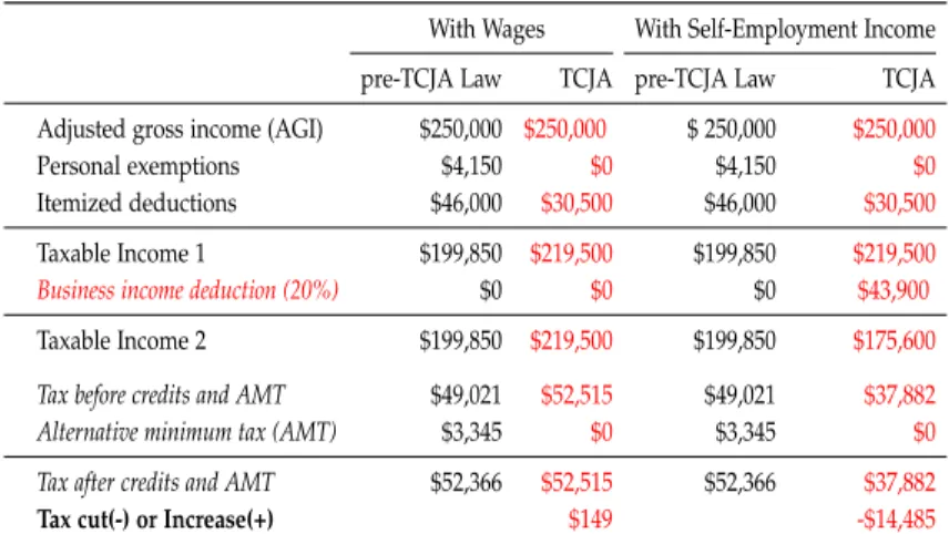
2.2 Illustrative exemple . . . 44

2.3 Model Economy . . . 45

2.3.1 Demographics and preferences . . . 45

2.3.2 Technologies. . . 46

2.3.3 Government and tax system . . . 48

2.3.4 Recursive formulation . . . 48

2.4 Calibration . . . 52

2.4.1 Preferences . . . 53

2.4.2 Demographics and endowments . . . 53

2.4.3 Technology and market arrangement . . . 56

2.4.4 Government and tax system . . . 56

2.4.5 Characteristics of the benchmark economy . . . 57

2.5 Effects of the TCJA: A long-run analysis . . . 59

2.5.1 Aggregate effects . . . 60

2.5.2 Entrepreneurial dynamics . . . 62

2.5.3 Distributional effects . . . 65

2.6 On the transitional path of the TCJA . . . 68

2.6.1 Aggregate activity . . . 69

2.6.2 Comparison with others estimates . . . 70

2.6.3 Activity in the entrepreneurial sector . . . 72

2.6.4 Welfare analysis. . . 74

2.7 Conclusion . . . 77

3 Optimal Business Income Taxation 78 3.1 Introduction . . . 78

3.2 Economic Environment . . . 82

3.2.1 Demographics and preferences . . . 82

3.2.2 Technologies. . . 82

3.2.3 Government and tax system . . . 84

3.2.4 Recursive formulation . . . 85

3.3 Calibration . . . 88

3.3.1 Preferences . . . 89

3.3.2 Demographics and endowments . . . 89

3.3.3 Technology and market arrangement . . . 92

3.3.4 Government and tax system . . . 93

3.4 Optimal taxation problem . . . 93

3.4.1 Optimal tax reform along the transition . . . 95

3.4.2 Optimality and Efficiency . . . 101

3.5 Discussion . . . 105

3.5.1 Financing with consumption tax . . . 106

3.5.2 Effect of entrepreneurial human capital . . . 107

3.6 Conclusion . . . 109

4 On the Corporate Tax Reform: Coordination and Trade-offs 111 4.1 Introduction . . . 111

4.2 Model Economy . . . 115

4.2.1 Household . . . 115

4.2.2 Firm . . . 116

4.2.3 Government . . . 118

4.2.4 Equilibrium and Qualitative results . . . 119

4.3 Quantitative analysis . . . 124

4.3.1 Calibration. . . 124

4.3.2 Benchmark Economy. . . 125

4.4 Transitional dynamics . . . 134

4.4.1 Corporate tax cuts with labor income tax adjustment . . . 134

4.4.2 Optimality with transition. . . 135

4.4.3 Government budget during transition . . . 138

4.5 Conclusion . . . 139

Bibliography 142

Annexes 152

4.6 Appendix of Chapter 1 . . . 152

4.6.1 Labor efficiency units and productivity shock . . . 152

4.6.2 Extended results on the empirical findings . . . 153

4.6.3 Robustness check with Selection bias . . . 154

4.7 Appendix of Chapter 2 . . . 156

4.7.1 Main forces : General Equilibrium vs. Partial . . . 156

4.7.2 Some details about key provisions as written in the Law and sensi-bility analysis . . . 157

4.8 Appendix of Chapter 3 . . . 161

4.8.1 Some results in the optimal steady-state regime . . . 161

4.9 Appendix . . . 163

4.9.1 Proof of proposition 2 . . . 163

4.9.2 Trade-offs without revenue neutrality . . . 165

4.9.3 Proof of lemma 1 . . . 167

1.1 Wealth-income ratio over the life-cycle. . . 9

1.2 Wealth and entrepreneurial experience . . . 9

1.3 Wealth , age and entrepreneurial experience . . . 10

1.4 Entrepreneurship by age . . . 30

1.5 Gini profiles . . . 33

1.6 Income Gini profiles by occupation. . . 34

1.7 Variance of log income . . . 35

2.1 Age distribution of firms . . . 64

2.2 Evolution of aggregate quantities . . . 69

2.3 Evolution of entrepreneurial variables I . . . 72

2.4 Evolution of entrepreneurial variables II . . . 74

2.5 Inequality and welfare gain . . . 75

2.6 Support for the reform . . . 76

3.1 Government’s discount factor and Optimality . . . 98

3.2 Evolution of aggregate quantities: Effect of the discount factor . . . 99

3.3 Inequality and welfare effect . . . 100

3.4 Opitmality as a function of Inequality aversion and discount factor: . . . . 102

3.5 Evolution of aggregate quantities in case of efficiency (ˆs = 0) . . . 104

3.6 Inequality and welfare effects . . . 105

3.7 Planner’s discount factor, optimality and consumption tax . . . 107

3.8 Planner’s discount rate, optimality and business experience . . . 109

4.1 Overview of tax revenues when reform 1 is implemented . . . 129

4.2 Optimal reform . . . 133

4.3 Reform 1 with corporate tax of 21% . . . 136

4.4 Reform 1 with corporate tax of 0% . . . 137

4.5 Optimal reform with transition . . . 137

4.6 Government deficit/surplus-output ratio during transition . . . 140

4.7 Labor efficiency unit over the life-cycle . . . 153

4.8 Cohort effect over the life-cycle . . . 154

1.1 Income function estimates for Entrepreneurs . . . 12

1.2 Entry (Logit estimation) . . . 14

1.3 Exit (Survival analysis) . . . 15

1.4 Fixed parameters . . . 24

1.5 Jointly calibrated parameters . . . 27

1.6 Goodness of fit . . . 28

1.7 Wealth and Income distribution . . . 32

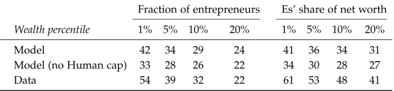
1.8 Entrepreneurs and the distribution of wealth (non targeted) . . . 32

1.9 Dispersion averages by occupation . . . 36

1.10 Dispersion averages by occupation mobility . . . 38

2.1 Single high-earner with wages or self-employment income . . . 45

2.2 Fixed parameters . . . 53

2.3 Jointly calibrated parameters . . . 56

2.4 Targets: Data and Model . . . 57

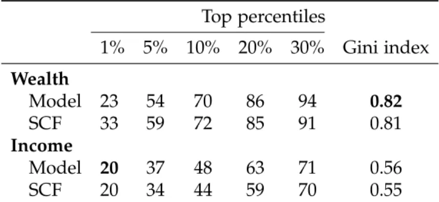
2.5 Wealth and Income distribution . . . 58

2.6 Fraction of Entrepreneurs by wealth percentile (non targeted) . . . 58

2.7 Tax Cuts and Job Act (TCJA): reform of 2017 . . . 59

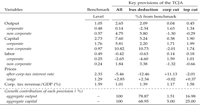
2.8 Aggregate effects of the TCJA . . . 60

2.9 Entrepreneurial statistics under the TCJA . . . 63

2.10 Entrepreneurial statistics by firm age under the TCJA . . . 65

2.11 TCJA and economic inequality (Gini index) . . . 66

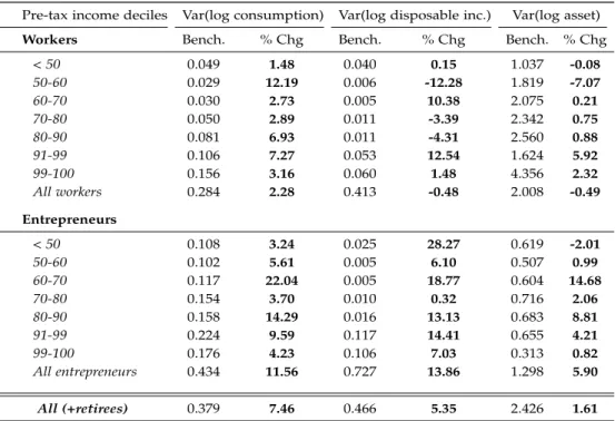
2.12 Inequality by occupation and income group . . . 67

2.13 Distribution of effective tax rate (%) . . . 68

2.14 Comparison of growth rates . . . 70

2.15 Welfare gain by occupation (%) . . . 74

3.1 Fixed parameters . . . 89

3.2 Jointly calibrated parameters . . . 92

3.3 Goodness of fit . . . 93

3.4 Aggregates under optimal flat rate regime (long run) . . . 95

3.5 Distribution of entrepreneurs across wealth . . . 97

3.6 Aggregate welfare gains and Support . . . 101

3.7 Welfare gain by occupation and wealth group (%) . . . 105

3.8 Aggregate welfare gains and support with consumption tax . . . 107

4.1 Benchmark calibration . . . 126

4.2 Elasticities and multipliers . . . 126

4.3 Multipliers . . . 128

4.4 Level change in tax rates (Reforms 1 to 3) . . . 131

4.5 Level change in tax rates (Reforms 4 to 7) . . . 132

4.6 Heckman two-stage correction model estimation . . . 155

4.7 Aggregate effects : 20% business income deduction’s case . . . 156

4.8 Entrepreneurial statistics: 20% business income deduction’s case . . . 156

4.9 Aggregate effects : top marg. tax cut’s case ( from 39.6!37%) . . . 157

4.10 Entrepreneurial statistics : top marg. tax cut’s case ( from 39.6!37% ) . . 157

4.11 Tax Cuts and Job Act (TCJA): reform of 2017 . . . 158

4.12 Aggregate effects of the TCJA in the long run . . . 160

4.13 Entrepreneurial statistics under optimal flat rate regime(steady state) . . . 161

4.14 Distribution of effective tax rate (%) . . . 161

Introduction

Entrepreneurship is a core activity in the U.S. economy. It is an opportunity for agents to take on risk and innovate, create jobs and output growth. Since this activity is risky and may lead to default, entrepreneurs face financial constraints and must rely on their personal wealth to start up or scale up their ventures. As a consequence, business owners have higher saving rates and end up at the top-end of the income and wealth distributions (Quadrini, 2000; Gentry and Hubbard, 2004; Cagetti and De Nardi, 2006). The U.S. data show that business owners represent more than half of the wealthiest one percent and hold 60% of the wealth, the resulting inequality gap oftentimes triggers redistributive tax policies. However, the incentive to pursue productive entrepreneurship could be dampened if the government tax policy is very progressive.

These policies can often be controversial in public debates since economic inequality is also a growing issue. On the other hand, the supply-side logic argues that a special treat-ment of business income alleviates financial constraints and incentivizes entrepreneurs to take on more risk by increasing investment and employment. Thus the economy will benefit from the indirect effects of this dynamics. Most business income is earned by privately held businesses or pass-through entities (Sole proprietorships, Partnerships, and S-corporations). They are taxed like salaried workers. Therefore, the effects of a separate treatment of business income and labor income under the personal income tax code need to be understood. For instance, four nordic European countries -Norway, Fin-land, Sweden and Denmark- since the early 90s experience a dual income taxation. In this Nordic system, labor income and capital are taxed separately. On average capital income is taxed at a flat tax rate corresponding to the marginal tax for the first bracket of the progressive income code (Cnossen, 1999). In the US, the new special deduction provision of 20-percent for business owners contained in the recent tax reform known as Tax Cuts and Jobs Act (TCJA) as of 2017 is an example of an early attempt of the differential tax treatment of business owners relative to salaried workers. The (optimal)

tax literature has been, however, almost silent on the issue of the separate taxation be-tween business income and labor income. This thesis purports to fill this gap through a positive investigation (chapter 2) and a normative analysis (chapter 3) after showing that occupation-specific human capital or business experience is supported by the data (chapter 1).

Moreover, the TCJA significantly altered how business income is taxed in the US in general. A major provision in this tax bill is the permanent reduction of the top statutory tax rate from 35% to 21% for corporate firms. Critically, the reform fails to meet the revenue neutrality condition since it adds $1.5 trillions to the current deficit over the next decade. Therefore, the last chapter of this thesis addresses the following question: How to finance a corporate tax cut? The potential loss of government revenue might be detrimental to safety net programs such as Medicaid and Medicare.

Specifically, Chapter 1 provides evidence using the PSID that occupation-specific hu-man capital or business experience is quantitatively important in explaining income and wealth disparities among individual over their life cycle. To capture the data patterns, I build on Cagetti and De Nardi (2006)’ occupational choice model, modified to fea-ture life-cycle dynamics. I also introduce managerial skill accumulation which leads entrepreneurs to become more productive with experience. I then calibrate two versions of the model (with and without accumulation of business experience) to same US data. Results show that the model with business experience margin is the closest one.

Chapter 2’s research question is timely to the recent tax reform enacted in the us, which is a major change of the tax code since the 1986 tax reform act. The Tax Cuts and Jobs Act (TCJA) as of December 2017 significantly altered how business income is taxed in the US. I then consider a dynamic general equilibrium model of entrepreneur-ship developed in Chapter 1 to provide a quantitative assessment of the macroeconomic effects of the TCJA, both in the short run and in the long run. The TCJA is modeled by its three key provisions : a 20-percent-deduction rate for pass-throughs, a drop in the statutory tax rate for corporations from 35% to 21% and the reduction to 37% of the top marginal tax rate for individuals from 39.6%. I find that the economy experiences, a GDP growth rate of 0.90% over a ten-year window and average capital stock increases by 2.12%. These results are consistent with estimates made by the congressional budget office and the joint committee on taxation. With temporary provisions, the TCJA delivers a reduction in wealth and income inequality but the opposite occurs once provisions are made permanent. In both scenarios, population suffers a welfare loss and finds them difficult to support.

Chapter 3 answers the normative question: Should entrepreneurs be taxed differently? Accordingly, I quantitatively investigate the desirability of an occupation-based taxation in the entrepreneurship model of Chapter 1, when transitional cohorts are explicitly taken into account. The main experiment is to move from the federal single progressive taxation for both labor income and business profit at the individual level to a differential tax regime where business income faces a proportional tax rate and labor income is still subject to the progressive scheme. I find that a tax rate of 40% is optimal. More generally, the optimal tax rate varies between 15% and 50%, increasing with the planner’s aversion to inequality and decreasing with its relative valuation of future generations’ welfare.

In the context of business tax reform, chapter 4 assesses revenue-neutral trade-offs when financing a corporate tax cut. To meet revenue neutrality, the policymaker uses three instruments to balance the government budget, namely labor income tax, dividend tax and capital gains tax. I then construct a parsimonious general equilibrium model to derive balanced fiscal multipliers associated with a corporate tax reform. Using a standard calibration, I find that when labor income tax or dividend tax are individually used to make up the corporate profit tax cut, the balanced fiscal multiplier associated to the labor income tax is positive and smaller than that of dividend tax rate. The positive sign for both instrument suggests that, if the policy maker reduces the corporate tax rate it should increase each of those instruments in some proportion given by the multiplier. On the other hand, the balanced fiscal multiplier with respect to the capital gains tax turns out to be negative. In this case, a corporate tax cut can be coupled with a cut in capital gains tax. Therefore, there is no trade-off in this scenario. Moreover, the welfare gains of the different scenarios are mixed.

Chapter 1

Unequal we stand: Human capital and

Occupational choice over the Life cycle

1.1 Introduction

There are large differences in the amount of wealth and income held by different house-holds in the US within-age and between age-cohorts; and any redistributive policy re-quires a good understanding of the drivers of such disparities with respect to individuals’ lifespan. Therefore, the question of what drives inequality over the life-cycle? is still an open question although it has been tackled by many studies using quantitative dynastic and life-cycle frameworks with different mechanisms at play (Huggett, 1996; Quadrini and Ríos-Rull, 1997;De Nardi and Fella,2017).

Entrepreneurship has been found to be very important in explaining large saving rates difference among households (Quadrini, 2000;Cagetti and De Nardi, 2006;Buera,2009). For instance, the higher return to capital in active businesses and financial constraints incentivize agents to save more before transitioning into or staying in entrepreneur-ship, and then they end up having higher wealth-income ratios and saving rates than non-entrepreneurial households on average. Accordingly, using the PSID I document that over the life cycle1 _{i) the age profile for wealth to income ratio is steeper for} en-trepreneurs, and ii) cumulative business experience is associated with higher income 1_{Quadrini(1999) points out the differences of wealth-income ratios between entrepreneurs and} work-ers using the PSID waves from 1984 to1994 with respect only to occupation not age. In a cross-sectional analysis of SCF 1989 dataGentry and Hubbard(2004) also document higher wealth-income ratio for en-trepreneurs by age-groups.

and wealth, favoring (re)entry and reduces exit. Furthermore, since occupational choice introduces mobility between entrepreneurship and salaried work over the life cycle, I an-alyze the data along this margin and find that iii) work-stayers have the lowest inequality and dispersion of income, iv) entrepreneur-stayers have as much inequality and income dispersion as switchers involving entrepreneurship.

To capture these patterns, I adopt a life-cycle model with occupational choice and uninsurable risk in both entrepreneurial and paid-work sectors. I also introduce man-agerial skill accumulation which leads entrepreneurs to become more productive with experience. The facts documented above suggest that the interconnection of occupa-tional choice and cumulative (business) experience might be potentially an interesting channel contributing to the inequality depicted in the data. In the model, agents are ex ante identical and go through their lifespan subject to idiosyncratic dynamics of work and entrepreneurial ability, and an exogenous age-profile earnings for workers. How-ever, provided that the occupational choice is endogenous and related to savings and realized entrepreneurial ability, two agents in a given cohort might not have the same income and wealth making heterogeneity within-cohort possible even without labor pro-ductivity shock. Another layer of heterogeneity arising endogenously in the model is the accumulation of human capital or business experience via a learning-by-doing process. This human capital could be interpreted as business acumen, know-how, book-keeping and so on, namely any kind of knowledge an individual might learn while being ex-posed to entrepreneurial activities. In fact, empirical studies find that entrepreneurship is experimentation allowing individuals to learn and increase their productivity or, even exit the business sector (Åstbro and Bernhardt, 2005; Amaral et al.,2011; Parker, 2013).

I find that entrepreneurial dynamics by age is consistent with the documented facts and the fit is overall better when human capital channel is considered. Since the model without entrepreneurial experience is calibrated to match the same target data moments as in the benchmark, the wealth and income distributions are almost similar in both mod-els for the whole population. As already shown in previous papers, the entrepreneurship motive which generates high saving rates for would-be entrepreneurs is important on its own. I then rely on non-targeted data moments to cast light on the marginal contribu-tion of cumulative business experience. The model with the learning-by-doing channel emerges as the closest one to the non-targeted data moments. For instance, adding the accumulation of entrepreneurial experience into the model without human capital in-creases the fraction of entrepreneurs in the top 1% of wealth distribution by 9 percentage point and their share of wealth by 7 percentage point. This increase is 6 percentage point

for the top 5% wealthy entrepreneurs. I therefore argue that the future rewards of human capital if entrepreneurs sustain their position long enough in the business sector is quan-titatively important in generating realistic dispersion among entrepreneurs. The main value-added of business experience introduced here is its capacity to bring the model that embodies it closer to the non-targeted data, specifically for entrepreneurs.

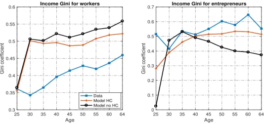
Using different inequality metrics I find that entrepreneurial-specific human capital via learning-by-doing is important in explaining income disparities between individuals with respect to occupation and age. Considering the variance of log income by occupa-tion and age, the human capital model predicts an increasing pattern over the life cycle for entrepreneurs, which is consistent with the empirical counterpart. However, absent human capital accumulation, the model fails after age 30 to account for this upward-sloping dispersion in the business sector. I find a net contribution up to 0.5 percentage point near retirement for the model with human capital. The variance of log income also shows that there is twofold dispersion between workers and entrepreneurs in the data and in the model with business experience while the alternative model displays as much dispersion for worker as for entrepreneurs.

I also examine the inequality at the bottom and the top of the income distribution using the log 50/10 and the log 90/50 ratios, respectively. I find that there is more inequality at the bottom than the top for both occupations in the data, but this is reversed in the two models. In fact, the PSID data oversample low-income households inducing the bottom half of the income distribution to be a driver of the inequality. On the other hand, the presence of entrepreneurship in both model leads agents to save more, which makes the top half a driver of the inequality.

This work is related to the vast quantitative literature of savings and wealth accumu-lation over the life-cycle. Castaneda et al. (2003) emphasize higher productivity level to deliver a realistic wealth distribution for the US economy while De Nardi (2004) focus on bequest motive and intergenerational human capital transfer mechanism. The im-portance of preferences heterogeneity is investigated by Hendricks(2007). In a life-cycle model with idiosyncratic human capital accumulation, Huggett et al. (2011) show that differences in initial conditions as of age 23 explain most of the lifetime inequality. In a recent contribution, De Nardi et al. (2016) revisit a life-cycle environment while taking advantage of a structural estimation of the earnings process using PSID and administra-tive data. Kaymak and Poschke (2016) show that the increasing wage dispersion is the main driver of income and wealth inequality over half a century in the US. The current setup considers a life-cycle model with entrepreneurship margin.

The occupational choice connects this paper to the strand of the literature showing the importance of entrepreneurship in describing the saving behavior of wealthy house-holds and the dynamics of wealth inequality (Quadrini,2000;Evans and Jovanovic,1989;

Gentry and Hubbard,2004; Hurst and Lusardi,2004). The entrepreneurial mechanism is extensively discussed for a variety of purposes such as effect of wealth on transition prob-ability into entrepreneurship (Hurst and Lusardi, 2004; Buera, 2006; Mondragón-Vélez,

2009), tax policy (Cagetti and De Nardi, 2009; Kitao, 2008; Meh, 2005), among others). My model highlights the endogenous business experience channel on inequality.

This paper also shares the intuition that the formal or informal human capital affects the labor market outcomes (Mincer, 1974; Becker,1975). For example,Roys and Seshadri

(2014) andGuner et al.(2015) show in an entrepreneurial choice model without financial constraint that human capital accumulation through schooling and on-the -job enhance workers-firm match quality. Investment in formal schooling is also a potential boost for entrepreneurship with trade-offs when there are borrowings constraints (Castro and Sevcik, 2016; Mestieri et al., 2016; Samaniego and Sun, 2016). On the other hand, human capital can be accumulated via experience or learning-by-doing process.2 _{The potential} of occupational-specific human capital in life-cycle economies without entrepreneurship explored inKeane and Wolpin(1997) four young in the NLSY 79 and inKambourov and Manovskii(2009) for workers’ wage inequality in the PSID.

The layout is as follows. Section 1.2 documents empirical facts that highlight the potential contribution of business experience in entrepreneurship dynamics and earnings over the life cycle. The model and its recursive formulation are presented in section 3.2. Section3.3 discusses model calibration whereas the quantitative results are presented in section 4.3.2. Concluding remarks are given in section1.6 concludes.

1.2 Evidence on entrepreneurial experience and inequality

I use the Panel Study of Income Dynamics (PSID) waves 1968-2011 and the Survey of 2_{Using bayesian mechanism about beliefs in entrepreneurial skills and firms dynamics, Jovanovic(1980)} gives an earlier theoretical contribution. Nonetheless, the empirical literature is grounded with mixed contributions of entrepreneurial human capital depending on how one defines it in the data. See (Åstbro and Bernhardt,2005; ?;Parker,2013;Toth,2014).

Consumer Finance (SCF 2010) data. I collect information on head of households (male and female) about economics outcomes (occupation status, annual labor income, annual hours worked, wealth) and demographics (age, sex, college degree). For the analysis below, I include households whose head i) is between 20-64, ii) and works positive hours. Income are transformed into 2011 US dollars using Consumer Price Index.

The notion of entrepreneur is a construct because there is no direct measure for it in the data. However, using the job status available in the data, I define an entrepreneur as individual who is actively managing his business (Cagetti and De Nardi, 2006).

Fact 1: The age profile for wealth to income ratio is steeper for entrepreneurs.

Since entrepreneurs rely more often on internal financing to start out with their en-deavors, their are likely to hold higher wealth as compared to non-entrepreneurs. This can be shown by using for example wealth-income ratios, saving rates and other relevant statistics. Figure1.1 shows the age-profile of wealth-income ratios among entrepreneurs and workers using two sets of data. One can notice two interesting patterns. First, the wealth-income ratio is upward sloping for both occupations over the life-cycle sug-gesting that agents accumulate more wealth while they age as is standard. The second trend is that, entrepreneurs’ wealth-income ratio is consistently higher than that of non-entrepreneurial households3 _{and, it rises approximately threefold from younger ages} to retirement. On average, the wealth-income ratio is 11.15 for entrepreneurs and 3.21 for workers using the PSID, while in the SCF 2010 one finds wealth-income of 10.66 for entrepreneurs and 3.65 for workers. Therefore, the overall differences between en-trepreneurs and workers could be investigated in the early stages of life and provide rationale to look at the inequality during the different stages of life. These facts are not only consistent over time since the first panel in figure 1.1 uses PSID data from 1984 to 2011, but also at the cross-sectional level provided that the use of SCF 2010 reveals a similar pattern in the second panel.

3_{Quadrini(1999) also finds similar results using three income classes with PSID data from 1984, 1989,} and 1994 without the age dimension. On average, he finds wealth-income ratio for entrepreneurs amount-ing to 5.9 while that of workers is 2.86. Gentry and Hubbard (2004) use SCF 1983 and 1989 data and document the higher wealth-income ratio by quintile for households becoming or staying entrepreneurs.

Figure 1.1: Wealth-income ratio over the life-cycle. 25 30 35 40 45 50 55 60 64 Age 0 5 10 15 20 25 30 35 Wealth-income ratio

Wealth-income ratio by age (PSID)

Entrepreneurs Workers 25 30 35 40 45 50 55 60 64 Age 0 5 10 15 20 25 30 35 Wealth-income ratio

Wealth-income ratio by age (SCF)

Note: In the first panel wealth and income are in 2011 US dollars and are computed as average by age before taking the ratio. Each dot represents an average over a five-year bin. The blue line is for entrepreneurs while the red one represents workers.

Fact 2: Cumulative business experience is associated with higher wealth and income. Figure 1.2: Wealth and entrepreneurial experience

0 .1 .2 .3 desnsity 0 5 10 15 20

wealth (log scale)

experience(1−5) years experience(6−10) years experience>10 years zero experience

Distribution of wealth by entrepreneurship experience

One advantage of using the PSID is that it allows one to trace out the entrepreneurship spell for individuals, thereby highlighting the existence of serial entrepreneurs -individuals who have been entrepreneur more than once. The cumulative experience

during a business tenure is an important human capital upon which an entrepreneur builds up his subsequent success. Figure 1.2 pinpoints the heterogeneity within the en-trepreneurial sector with respect to entrepreneurship spell. It can be readily seen that the wealth distribution is shifting towards the right with a higher average for more experi-enced entrepreneurs.

Given that even in the same age-cohort, individuals may not have the same en-trepreneurship spell, figure1.3plots the average wealth of three age groups with respect to experience. Thus, controlling for entrepreneurs’ age shows that wealth increases with accumulated business tenure in almost all age group. I interpret these facts as evidence for accumulation of skills that are pertinent for effectively running one’s business. How-ever, the apparent facts depicted here may be artifacts that stems from intrinsic charac-teristics pertaining to individuals and/or the longitudinal nature of the data. Therefore, I make further analysis by estimating an income function for entrepreneurs4_{and control} for these potential biases.

Figure 1.3: Wealth , age and entrepreneurial experience

0 5 10 15 20 25 30 Years of entrepreneurship 4.8 5 5.2 5.4 5.6 5.8 6 6.2 6.4 6.6 6.8

Mean wealth (log scale)

Wealth by entrepreneurial experience and age

55 years old 45 years old 35 years old

I estimate the following income function:

lneit = y1Ait+ y2A2_it+ y3Colit+ y4Expit+ y5Exp2_it+ ui+ µt+ zit (1.1) 4_{One might suggest that a better statistic would have been earnings or business income instead of total} income. While I acknowledge the relevance of this concern, the non-availability of this data in the PSID justifies the use of total income. Indeed, in the PSID, the business income for entrepreneurs is part of the total labor income of the head of the household in almost all the different PSID waves under consideration in this paper. Accordingly, business income is identified by the occupational status of the head of the household. Therefore, in this section I shall use these two concepts interchangeably.

where e_it is the real annual income of entrepreneur i in period t, A_i is individual’s age, Exp is the cumulative years of entrepreneurship up to time t and controls for the en-trepreneurial human capital accumulation. Since formal education is another channel to enhance one’s skills, it may be the case that more educated entrepreneurs are prone to be persistent in the business sector. Therefore, variable Col is a dummy variable capturing this fact and takes value one if an individual has a college degree and zero, otherwise. Individual idiosyncratic characteristics rather than what explicitly outlined above are in-cluded in ui, also the aggregate economic environment’s impact is controlled for by µt. The variable zit is the error term with the standard exogeneity assumption .

The results are summarized in table 1.1. The first two columns show the standard effects of age on the earnings process. That is the earning function is not linear with respect to age suggesting a decline after a certain age in the life course. Education al-lows an entrepreneur to increase his earnings (Column 2), the entrepreneurial experience could play a substitute role as indicated in column 3. In column 4 where the full model is estimated, the accumulated experience in the business sector is still statistically signif-icant in the earning. The presence of education barely changes its contribution. Roughly, one more year of entrepreneurship increases the earnings by 5%.5 _{This result provides} an empirical support for including entrepreneurial human capital accumulation in terms of year of experience as an important driver of entrepreneurship dynamics.6

5_{This result is in line with findings in Kambourov and Manovskii (2009) and Toth (2014). Indeed,} Kambourov and Manovskii(2009) show that, else being equal, 5 years of occupational tenure are associated with an increase in wages of 12% - 20% in the U.S. economy using the PSID. In a randomized experiment with Indonesian data,Toth(2014) finds that on average, an extra year of experience causes a 3% increase in net profit.

6_{This result is robust to the potential selection bias relative to occupation. In fact, I implement a} two-stage Heckman correction model where I use the demeaned of total business experience at the individual level and its squared values as supplementary predictive variables for the selection probability. The choice of these instruments follows the approach in Altonji and Shakotko (1987). See Appendix 4.6.3 for the robustness check results.

Table 1.1: Income function estimates for Entrepreneurs

Log income (1) (2) (3) (4)

loginc loginc loginc loginc

Age 0.125⇤⇤⇤ _0.103⇤⇤⇤ _0.101⇤⇤⇤ _0.088⇤⇤⇤ (0.026) (0.011) (0.0278) (0.012) Age2 _0.001⇤⇤⇤ _0.001⇤⇤⇤ _0.001⇤⇤⇤ _0.001⇤⇤⇤ (0.0001) (0.0001) (0.0001) (0.0001) College 0.289⇤⇤⇤ _0.289⇤⇤⇤ (0.041) (0.041) Business experience 0.054⇤⇤⇤ _0.049⇤⇤⇤ (0.122) (0.009) Business experience2 _0.001⇤⇤ _0.001⇤⇤⇤ (0.0004) (0.0004) Constant 8.123⇤⇤⇤ _8.344⇤⇤⇤ _8.964⇤⇤⇤ _8.930⇤⇤⇤ (0.580) (0.227) (0.635) (0.257) Observations 11236 11236 11236 11236 R-squared 0.052 0.048 0.056 0.052 Number of entrepreneurs 2754 2754 2754 2754

Individual Fixed Effects _{X X}

Year Fixed Effects X X X X

Note: Income is total labor income data from PSID 1968 to 2011 in 2011 US dollars. Age is the age of the head of household, business experience equals the cumulative years of entrepreneurship up to period t, college is a dummy variable and an entrepreneur is a self-employed and business owner. Robust standard errors are reported in parentheses and the significance level defined as:⇤10%;⇤ ⇤5%;⇤ ⇤ ⇤1%.

Fact 3: Entrepreneurship experience has predictive power on income and wealth, favors (re)entry and reduces exit rate.

Next, I estimate the impact of past business experience on entry to and exit from entrepreneurship. I fit the data with a Logit model with fixed effects for entry and re-entry and apply a survival analysis to the exit process. I show the results in table1.2and

1.3, respectively. Columns 1 and 3 in table 1.2 reveal that wealth and tenure positively affect (re)entry probability. The intuition behind this result is that wealth allows a would-be entrepreneur to get rid of external financial constraints to launch his venture, and previous entrepreneurial experience helps build up some confidence which incentivizes the entrepreneur to take on more risk. The existence of serial entrepreneurs in the data may be partially explained by this factor. The contribution of each factor or odds ratio is reported in columns 2 and 4, it gives the extent by which entry probability is increased with respect to each variable. For instance, a one-year tenured entrepreneur has 3 times more likely to re-enter into entrepreneurship than a would-be entrepreneur. This number is even higher than the one implied by wealth.

Table 1.2: Entry (Logit estimation)

(1) (2) (3) (4)

Entry Odds ratio Entry Odds ratio

Age 0.0644⇤⇤⇤ _1.066⇤⇤⇤ _0.0561⇤⇤⇤ _1.0576⇤⇤⇤ (0.0176) (0.0187) (0.0174) (0.0184) Age2 _0.001⇤⇤⇤ _0.998⇤⇤⇤ _0.001⇤⇤⇤ _0.998⇤⇤⇤ (0.0002) (0.0002) ( 0.0002) (0.0002) College 0.344⇤⇤⇤ _1.412⇤⇤⇤ _0.227⇤⇤⇤ _1.254⇤⇤⇤ (0.084) (0.1185) (0.0839) (0.105) Business experience 1.187⇤⇤⇤ _3.279⇤⇤⇤ _1.157⇤⇤⇤ _3.181⇤⇤⇤ (0.0253) (0.0831) (0.0250) (0.0795) Business experience2 _0.037⇤⇤⇤ _0.963⇤⇤⇤ _0.037⇤⇤⇤ _0.964⇤⇤⇤ (0.0011) (0.0010) (0.0011) (0.0010) Wealth 0.044⇤⇤⇤ _1.045⇤⇤⇤ (0.0038) (0.0040) Wealth2 _0.001⇤⇤⇤ _0.999⇤⇤⇤ (0.00001) (0.00001) Constant 5.306⇤⇤⇤ _0.005⇤⇤⇤ _5.066⇤⇤⇤ _0.006⇤⇤⇤ (0.3812) (0.0019) (0.3779) (0.0024) Observations 52443 52443 52443 52443

Year Fixed Effects X X X X

Likelihood ratio 1427.70 1427.70 1256.02 1256.02

Note: PSID data from 1984 to 2011. Wealth is family wealth in 2011 US dollars divided by 100,000. Age is the age of the head of household , college is a dummy variable, business experience equals the cumulative years of entrepreneurship up to period t and an entrepreneur is a self-employed and business owner. Robust standard errors are reported in parentheses and the significance level defined as:⇤10%;⇤ ⇤5%;⇤ ⇤ ⇤1%. An odds ratio greater than one suggests that the corresponding control increases (re)entry likelihood, otherwise it is a fall.

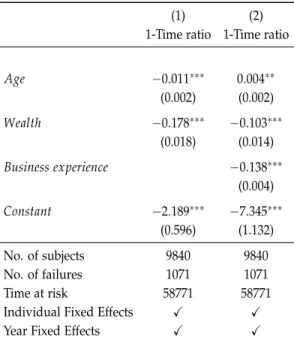
The hazard rate of failure or exiting entrepreneurship decreases with wealth and ex-perience as indicated in table 1.3. Intuitively, given that entrepreneurship requires more internal financing, then the wealthier the entrepreneur the easier it is to self-finance and overcome borrowing constraints, and hence stay much longer in entrepreneurship. The

tenure or business experience per se helps entrepreneur to have some business acumen and the like to quickly turns things around and adapt. This strength may incentivize individual not to exit. The time ratio gives more details in the contribution of each vari-able. Accordingly, one year of entrepreneurial experience reduces the exit probability by a factor of 14%, which slightly above that of 1% increase in one’s wealth. Therefore the impact of experience on the exit dynamics is non negligible .

Again, these facts not only emphasize the well-known importance of wealth in en-trepreneurship dynamics but, also highlight the complementarity effect of entrepreneurial experience.

Table 1.3: Exit (Survival analysis)

(1) (2)

1-Time ratio 1-Time ratio

Age 0.011⇤⇤⇤ _0.004⇤⇤ (0.002) (0.002) Wealth 0.178⇤⇤⇤ _0.103⇤⇤⇤ (0.018) (0.014) Business experience 0.138⇤⇤⇤ (0.004) Constant 2.189⇤⇤⇤ _7.345⇤⇤⇤ (0.596) (1.132) No. of subjects 9840 9840 No. of failures 1071 1071 Time at risk 58771 58771

Individual Fixed Effects X X

Year Fixed Effects X X

Note: PSID data from 1984 to 2011. Wealth is log of family wealth in 2011 US dollars , age is the age of the head of household, business experience equals the cumulative years of entrepreneurship up to period t and an entrepreneur is a self-employed and business owner. Robust standard errors are reported in parentheses and the significance level defined as: ⇤10%;⇤ ⇤5%;⇤ ⇤ ⇤1%. If (1-time ratio) is less than zero, then the corresponding control negatively affects Exit or increases survival. Otherwise, the reverse holds.

1.3 Model Economy

I build on Cagetti and De Nardi (2006) to allow individuals to choose occupation be-tween paid-work and entrepreneurship. However, the simple life-cycle structure in their model does not enable one to fully describe the transition in and out of entrepreneurship. Therefore I adopt a life-cycle approach with lifetime uncertainty but without bequests. They work for the first R years followed by an inactive period of retirement. Individuals live J periods and start their life with zero initial wealth.

1.3.1 Demographics and preferences

The economy is inhabited by multiple cohorts of individuals of different ages. Each cohort is comprised of a continuum of measure one of individuals who live for a finite number of periods. Each period, an agent of age j decides whether to be an entrepreneur or a worker. Agent of age j maximizes the expected flow of utility given by

E₀ " _J

Â

1.3.2 Technologies

Work productivity

Labor supply is inelastic. A worker earns a market wage w per efficiency unit of labor

e_j, where e_j denotes an age-specific productivity, which captures the average wage

be-tween workers of different age, and evolves deterministically along the life-cycle. Work-ers are also subject to idiosyncratic shocks, h, that are distributed according to the fol-lowing stochastic AR(1) process.

lnht = rlnht 1+ eh,t where eh,t sN(0, sh2)

Entrepreneurial experience

The more time an agent spends in the business sector, the more productive he be-comes as an entrepreneur experience rises, making the entrepreneur’s human capital an

essential input for the business to succeed. I define business experience at any age j by the total number of years an agent has worked as an entrepreneur in their career. Formally, let o(a, z, , h, j, k)_{2 {}worker, entrepreneur_}denote the occupational choice given asset, abilities, age j, and entrepreneurial experience k, the accumulation of this experi-ence is as follows k0 = k + 1_{{o(a,z,h,j,k)=e}}, (1.3) where 1= ( 1 if o(a, z, h, j, k) = entrepreneur 0 otherwise (1.4)

Effective entrepreneurial skill

The agent launches his business with the cumulative experience acquired previously. Accordingly, the productivity in the business sector is now determined endogenously. To capture the risky nature of entrepreneurial activity I consider a stochastic entrepreneurial ability z following a Markovian process. Therefore, the business income of any en-trepreneur might fluctuate. Let ze denote the effective entrepreneurial skill at time t as

ze = zkq, q 2(0, 1) (1.5)

ze is the effective entrepreneurial ability by which production will be carried out in the business sector and has the same stochastic process as the underlying z, and q is the elasticity of the effective human capital with respect to experience.

Entrepreneurial production

The production technology available in the entrepreneurial sector is in line with the span-of-control assumption (Lucas Jr, 1978). The entrepreneur rents working capital k at interest rate r and labor input l at market wage w in a constrained financial market environment. Markets arrangement are such that, the entrepreneur is able to borrow only up to a fraction l 1 of his initial wealth. Capital depreciates at rate d. Denoting the business income of the entrepreneur by p we have

p(a, z, k) = max

l 0, klazk

where a, g,₂(0, 1). Solving for interior solution along with concavity property of the profit function one obtains optimal size of the firm as

k⇤ _{= min} ( la, (gazkq)1 g1 " (1 a)(r + d)1 g(1 a)1 aw #g(1 a) 1 g ) (1.7) (1.8) l⇤ noconstr= (1 a_a)(r + d)_w k⇤ (1.9) l⇤ constr = " g(1 a)z_ek⇤ag w # 1 1 g(1 a)

The corresponding profit functions are given by

pnoconstr(a, z, h) = (1 g)(ze) 1 1 g " g(1 a) w #g(1 a) 1 g " ag r + d # ag 1 g (1.10) and

pconstr(a, z, h) = (1 g(1 a))(ze) 1 1 g(1 a) " g(1 a) w # g(1 a) 1 g(1 a) (la)ag _{(r + d)la (1.11)}

Equation 1.7shows the non-convexity in the optimal capital demand due to the borrow-ing constraint faced by the individual entrepreneur. The first part gives the constrained demand i.e. when the borrowing constraint is binding, therefore the size of the firm is tied to the business owner’s wealth. By contrast, the second term defines the uncon-strained optimal size that the entrepreneur can choose. The corresponding labor demand and profit when entrepreneur is not constrained is given in1.8and 1.10while that of the binding situation is set in 1.9and 1.11.

Non-entrepreneurial sector:

Not all businesses in the economy are performed by individual entrepreneurs. There is also a group of relatively large and unconstrained firms which I refer to as corpora-tions. I then suppose that these corporations are represented by a single corporate firm

using a constant-returns-to-scale production function. To capture the effect of corporate taxation, the aggregate corporate firm pays a proportional corporate tax tc on its operat-ing profit which is defined as production net of labor cost and capital depreciation.7 _The corporate firm then solves the following:

max Kc,Lc>0AcK

a

cL1 ac (˜r + d)Kc wLc (1.12)

with ˜r = r/(1 tc)

First order conditions give rise to

(1.13) ˜r + d = aAc K_Lc c !a 1 (1.14) w = (1 a)Ac K_Lc c !a

1.3.3 Government and tax system

Government levies proportional taxes on consumption(sales tax) Ts = tsC, progressive

taxes on personal income Ty and uses the proceeds to finance an exogenous outlay G

and retirement benefits, B. I consider the below tax scheme on income.

(1.15) yd = x min{ytop, y}1 t+ (1 tmax) max{0, y ytop}

(1.16) t(y) = y yd

where yd _{is agent’s disposable income, y the total income and t(y) the amount of tax} collected. The first term in equation 3.8 captures the progressivity of the U.S. personal income tax which can be approximated by a log-linear function outside the top income bracket8 _{(Benabou, 2002; Heathcote et al., 2014a; Bakı¸s et al., 2015). The second term}

7_{Indeed, operating profit is expressed as ˜p = AcK}a

cL1 ac dKc wLc. One can then show that tc˜p = tc˜rKc. Thus, the before-corporate tax is given by ˜r = r/(1 tc). Moreover, setting the interest rate in this way prevents pass-through entities to be subject to the corporate taxation (double taxation), which is consistent with the actual U.S. tax code.

8_{This tax schedule rules out lump-sum transfers but allows agents to receive tax rebates or transfers as} long as their total income y2(0, x1t).

represents the tax liabilities of those individuals in the top end of income distribution with tmax the top marginal tax rate (Kaymak and Poschke, 2016). The income level ytop is the critical level equalizing the marginal tax rates. That is, 1 x(1 t)y_topt = tmax. The tax system progressivity is captured by t. Accordingly, if 0 < t < 1 taxation is

progressive, meaning an increase in marginal tax with respect to income. A regressive

schedule, on the other hand, occurs when t < 0. The parameter x in equation 3.8

represents the average level of taxation in the economy and it also allows one to balance the government’s budget at the equilibrium. Each period government’s budget balances as

(1.17) G + B = Ts+ Ty+ tc˜rKc

1.3.4 Recursive formulation

Households maximize the expected flow of utility given in 3.2.1. I assume no aggregate uncertainty and prices are constant in the steady state.

Each period, an age-j individual starts with an initial wealth a, productivity h, en-trepreneurial ability z, experience k, and then chooses his current occupation. Work-ers earn income from labor, make consumption and savings decision. Entrepreneurs choose the working capital and labor input demand subject to the collateral constraint. Moreover, the entrepreneur gains one period of experience which will be essential in his subsequent ventures.

Agent’s problem a-Retiree’s problem

After retirement, agents live off their savings and retirement benefits (b). Pension is paid out to any retiree regardless of his pre-retirement occupation. The problem of a retired agent for ages j2 {R, R + 1, . . . , J} is given by

v_j(a) = max a0 ( u(c) + bv_j+1(a0₎ ) (Pr) (1.18) yr = ra + b (1 + ts)c + a0 = yd(yr) + a (1.19) a 0 (1.20)

v_J+1(a) = 0 (1.21) Thus, during the retirement agent just chooses his next period asset holdings. To the ex-tent that the agent’s lifetime ends at J, equation 3.14gives the one period ahead terminal utility which is zero. Recall that yd_{(.) is the net-of-tax schedule given in3.8.}

b-Working agent’s problem

Before retirement, any agent in the economy has the following choice: vj(a, z, h, k) = max

n

vw_j (a, z, h, k), ve_j(a, z, h, k)o (1.22) where vw

j (a, z, h, k) and vej(a, z, h, k) are the value functions of worker and entrepreneur, respectively.

b1-Worker’s problem

Conditional on being on the labor market, an age-j worker solves the following recur-sive problem by choosing next savings and occupation.

vw_j (a, z, h, k) = max a0 ( u(c) + b

Â

The expectation is taken with respect to the underlying Markovian productivity dis-tribution y(z0_{, h}0_{|z, h) for the two abilities with the assumption that they are not}

corre-lated.9 _{The worker’s income stems from efficiency unit of labor per market wage. The} budget constraint in (3.17) states that although the agent is bestowed with a given en-trepreneurial productivity z, his current income does not depend on this productivity because he has chosen to be a paid-worker anyway. However, in a forward-looking fash-ion, he knows that the next period entrepreneurial talent is subject to the evolution of 9_{This assumption is also made inCagetti and De Nardi(2006). They compute a robustness check with} correlated abilities but results are not affected.

the current productivity endowment, and so is his next occupation. Put differently, any agent in the model is a potential entrepreneur until he decides not to be one. Agent’s next period savings are bounded below given that agent is prevented to roll over debt, namely net wealth is non-negative. Provided that a worker does not carry out production tech-nology for his own, he does not accumulate this specific entrepreneurial experience.10 The equation3.18 then shows the static accumulation of entrepreneurial skill.

b2-Entrepreneur’s problem

The recursive problem of an entrepreneur is now stated as follows ve_j(a, z, h, k) = max a0 ( u(c) + b

Â

The main differences between the two occupations are the income earned in the cur-rent period and the accumulated human capital. In fact, the profit function p(.) is a com-plex function which incorporates the borrowing constraints faced by the entrepreneur as described in section 3.2.2. The occupation-specific human capital gained in the business sector is defined in Eq (3.22) and translates the learning-by-doing process embedded in entrepreneurship. Hence, it is a latent variable behaviorally determined.

Equilibrium

At each point in time, individuals differ from one another with respect to age j and to state s = (a, z, h, k, o) i.e. asset holdings a, entrepreneurial productivity z, work productivity h, entrepreneurial experience k and occupation o 2 {W, E, Retiree}. Let 10_{One could possibly think of a similar occupation-specific human capital accumulated in paid-work} sector. This extension not only will increase the computation burden but also will not change the intuition carried over by the current setup. Indeed, one could take the relative of the two human capital and then normalize the paid-working one rendering models equivalent. On the other hand, one could also argue that, since the model explicitly keeps track of the labor efficiency unit, the human capital in the paid-work sector is somehow taken into account.

a ₂ A = R+, z 2 Z, h ₂ H, k ₂ K and o ₂ O, and S = A x Z x H x K x O the entire state space. Let (S,_F(S), fj) be a space of probability, where _F(S) is the Borel s-algebra on S: for each _{B ⇢ F}(S), f_j(_B) denotes the fraction of agents aged j that are in_B. Given the age j distribution f_j, Q_j(s,_B) induces the age j + 1 distribution f_j+1 as follows. The function Q_j(s,B) determines the probability of an agent at age j and state s to transit to the set B at age j + 1. The policy function for savings, consumption, entrepreneurial capital and entrepreneurial labor is given by ga

j(s), gcj(s), kj(s) and lj(s), respectively.

Definition . Given a tax structure{t_s, t_c, t_I, t_max, x, b_}, a stationary recursive competitive

equilibrium is a set of functions {vw_j , ve_j, vj, ga_j, gc_j, kj, lj(s)}J_j=1, and prices {˜r, w}such that (i) given prices, the functions solve the household problem in (Pw), (Pe) and (3.15);

(ii) the prices satisfy the marginal productivity conditions i.e. ˜r = F_Kc(Kc, Lc) d and w = FLc(Kc, Lc);

(iii) capital and labor markets clear : R 1

Â

Â

Â

Â

f_j+1(_B) =

Z

SQj(s,B)dfj,8B ⇢ F(S); (v) the government balances its budget:

G + B = tc ₁ r tc ! Kc+ ts J

Â

Â

where yd

j = x min{ytop, yj}1 t+ (1 tmax) max{0, yj ytop} y_j= 1_{{occup=worker}}yw

j + 1{occup=entrepreneur}yej+ 1{Retiree}yrj.

1.4 Calibration

In this section, I discuss the parametrization of the model economy. The calibration procedure is then carried out in two steps: I first consider a set of fixed parameters drawn upon the literature (table1.4) and thereafter I jointly calibrate the remaining parameters so that the model economy is consistent with a set of aggregate statistics of the US.

economy (table 1.6). I use the PSID (1968-2011) and the SCF (2010) to compute some

relevant statistics.

Table 1.4: Fixed parameters

Parameter Symbol Value Source

Preferences, demographics and technology

Risk aversion s 2.0 Conesa et al.(2009)

Lifetime J 61.0 Average US data

Retirement R 46.0 Average US data

Corporate capital income share a 0.33 Gollin(2002)

Depreciation rate d 0.06 Stokey and Rebelo(1995)

Technology parameter Ac 1.00 Normalization

Borrowing limit l 1.50 Kitao(2008)

Labor productivity

productivity and process h, Ph See Appendix4.6.1 Storesletten et al.(2004)

Age-dependent efficiency unit {ej} See Appendix4.6.1 own estimate using PSID

Government

Government spending G/Y 0.17 Conesa et al.(2009)

Replacement rate trep 0.40 Kotlikoff et al.(1999)

Consumption tax ts 0.05 Imrohoroglu and Kitao(2010)

Tax progressivity t 0.17 Bakı¸s et al.(2015)

Top marginal tax tmax 0.396 US data

Deduction rate for entrepreneurs t_d 0.00 US data

Average effective corporate tax rate tc 0.29 Gravelle(2014)

1.4.1 Preferences

The relative risk aversion parameter s is set to 2 following Conesa et al. (2009). The subjective discount factor b is jointly set to 0.951 so that, in equilibrium, the capital-output ratio is 2.65.