Laboratoire d'Analyse et Modélisation de Systèmes pour l'Aide à la Décision CNRS UMR 7024
CAHIER DU LAMSADE
261
Juillet 2007
Better differential approximation for symmetric TSP
Bruno Escoffier, Jérôme Monnot
Better differential approximation for symmetric TSP
Bruno Escoffier∗ J´erˆome Monnot∗
July 3, 2007
Abstract
In this paper, we study the approximability properties of symmetric TSP under an approximation measure called the differential ratio. More precisely, we improve up to 3/4 − ε (for any ε > 0) the best differential ratio of 2/3 known so far, given in Hassin and Khuller, “z-Approximations”, J. of Algorithms, 41(2), 429-442, 2001.
Keywords: Approximation algorithm; Differential ratio; Traveling salesman problem.
1
Introduction
Due to both its practical and theoretical interests, symmetric TSP is one of the most fa-mous combinatorial optimization problems. Given a complete edge-weighted graph, one seeks a tour (Hamiltonian cycle) either of minimum length (MinTSP) or maximum length (MaxTSP). Shown to be N P -hard in the very early development of the complexity theory ([24]), it has been widely studied since then from an approximate point of view. A polyno-mial algorithm A is said to be ρ-approximate if for any instance I, m(A(I)) ≤ ρ opt(I) for a minimization problem (resp. m(A(I)) ≥ ρ opt(I) for a maximization problem), where m(x) denotes the value of the solution x of I, and opt(I) the optimum value of I.
While MinTSP is not 2p(n)-approximable where n = |V |, for any polynomial p, if P 6= N P , MaxTSP is in APX : the well known 3/4-approximation algorithm by Serdyukov [29] has recently been slightly improved up to 61/81 in [8], or even 25/33 using a random-ized algorithm [22]. Many classical subcases have been studied, the most famous being the so-called metric case, restriction where the weights satisfy the triangle inequality. Using this assumption, Christofides devised in [9] a 3/2-approximation algorithm for MinMetricTSP, and this is up to now the best ratio obtained. Dealing with MaxMetricTSP, the 3/4-ratio that holds for the general case can be improved up to 17/20 [8], or even 7/8 using a ran-domized algorithm [23]. Note that all these problems do not admit approximation schemes if P 6= N P [28].
In this article, we further study the approximation properties of symmetric TSP, but using another measure of the quality of a solution called the differential ratio. The differ-ential ratio of a solution x of value m(x) is defined as δ(x) = opt(I)−wor(I)m(x)−wor(I), where opt(I) is the value of an optimum solution, and wor(I) is the value of a worst solution. For instance, if one studies MaxTSP, then a worst solution is a minimum length tour. In other words,
∗
CNRS-LAMSADE, Universit´e Paris-Dauphine, Place du Mar´echal De Lattre de Tassigny, F-75775 Paris Cedex 16, France. E-mail: {escoffier,monnot}@lamsade.dauphine.fr
this ratio measures the relative position of m(x) in the interval [wor(I), opt(I)] containing all feasible values (the definition can be rephrased for a maximization problem as : the solution x is δ-approximate if m(x) ≥ δ opt(I) + (1 − δ)wor(I)). Of course, δ ∈ [0, 1] (0 for wor(I) and 1 for opt(I)), and the closer to 1 the better the solution. The main property of this ratio is to be stable under affine transformation of the objective function (see [14] for a mathematical and operational justification of the ratio). Introduced in [2, 3], this ratio has been first used for studying mathematical programming problems, where the standard ratio is not suitable when very common operations such as “removing a constant” are performed, see for instance [31]. Afterwards, this approach has been considered for the main combina-torial optimization problems, leading to the development of new techniques and interesting results (see for instance [5] for vehicle routing, [20] for several results on graph problems, [10, 15, 17] for MinColoring, [21] for several weighted versions of graph partitioning, [12, 13] for Bin Packing, [7, 16] for satisfiability, [11, 6] for Set Cover, and very recently [18] for weighted Set Cover, etc.). A survey of many results about differential approximation can be found in the book chapter [4].
Dealing with symmetric TSP, we shall point out two major differences when using the differential ratio instead of the standard one. First, the dissymmetry between maximizing and minimizing completely disappears. More precisely, using an affine transformation of weights (w(e) → w′(e) = M − w(e), for a sufficiently large M , as for instance the heaviest weight plus 1), one can easily see that solving MinTSP (resp. MaxTSP) with the initial weights is equivalent to solve MaxTSP (resp. MinTSP) on the transformed weights. Indeed, the value of any tour T verifies w′(T ) = nM − w(T ). Since the differential ratio is stable under affine transformation, this means that a δ-approximation algorithm for MinTSP (resp. MaxTSP) can be immediately derived from a δ-approximation algorithm for MaxTSP (resp. MinTSP).
The other difference, maybe rather surprising, is the equivalence between the metric case and the general case. While considering a metric distance is a rather important assumption when using the standard ratio, TSP and MetricTSP are equivalent when using the differ-ential ratio. Indeed, again, one only has to affinely transform weights w(e) → wM + w(e), where wM is the weight of an heaviest edge, to get an equivalent metric instance of sym-metric TSP.
To sum up, dealing with differential approximation ratios, MinTSP, MaxTSP, Min-MetricTSP and MaxMin-MetricTSP are all equivalent. These problems have been tackled sev-eral time from a differential approximation point of view. The best ratio obtained so far is 2/3 ([20, 25]), which can be improved up to 3/4 when the weights are restricted to be 1 or 2, [27] (note that in this case the best ratio known for the standard ratio is 7/6, see [28]). Let us also mention that classical optimization strategies have been studied, such as the well known local 2-opt which has been shown in [26] to be a 1/2-differential approximation (while not being a constant standard approximation algorithm even for MinMetricTSP). Note that, as well as in the standard approximation framework, these problems do not admit differential approximation schemes. Finally, dealing with asymmetric TSP, the best differential ratio obtained so far is 1/2 [20].
In this article, we improve these results by showing that symmetric TSP (i.e. MinTSP, MaxTSP, MinMetricTSP and MaxMetricTSP) is differential approximable within an asymp-totic ratio of 3/4 (more precisely within a ratio of 3/4 − O(1/n)). Note that this is a notice-able improvement respect to 2/3 also because this is very close to the best ratio known for
MaxTSP (61/81). Since for a maximization problem the differential ratio is smaller than the standard one (m(x) ≥ δ opt(x) + (1 − δ)wor(x) implies m(x) ≥ δ opt(x), when solution values are nonnegative), the gap is now almost as small as it can be.
Let us already mention that, carrying on with this line of research, the study of sym-metric TSP in the geosym-metric case seems to be of particular interest. Indeed, when vertices are points in the plane (and the weight is the Euclidean distance), then it has been shown that both MaxTSP and MinTSP admit an approximation scheme (see resp. [30] and [1]). The existence of a differential approximation scheme is undoubtedly a very interesting and challenging question that would deserve further research.
In the following, we denote by opt(I), apx(I) and wor(I) the value of an optimal, an approximate and a worst solution respectively for an instance I. Due to the equivalence between MaxTSP and MinTSP, the results, only proven for MaxTSP, are obviously also valid for MinTSP. The proof of the result of the paper consists of two parts : in Section 2 we devise a 3/4-differential algorithm when the number of vertices is even. In Section 3, we show that the general case reduces to the previous subcase obtaining asymptotically the same ratio (3/4 − O(1/n) in our case).
2
Approximation for even instances
In this section, we assume that the number of vertices is even (ie |V | = 2n), and provide a 3/4-differential approximation for symmetric TSP.
The method used is based on the computation of a maximum weight 2-matching E2 = {C1, . . . , Cp} of I = (K2n, w), which can be done in polynomial time, [19]. We separate two cases depending on the existence of a cycle of size 3 in E2.
Case 1: There exists j ∈ {1, . . . , p} such that |Cj| = 3. Wlog, assume that j = p and Cp = {v1, v2, v3}.
We present a heuristic which is an adaptation of the Serdyukov’s algorithm working for MaxTSP, [29].
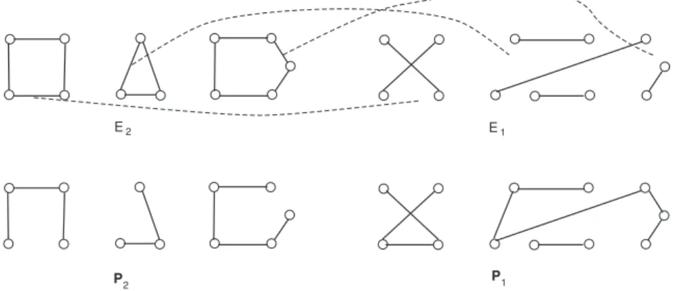
Let us first remind this algorithm and the result that can be derived from it (Lemma 2.1). This method consists in computing a maximum weight perfect matching E1 of I and moving one edge of each cycle Ci of E2 to E1 in such a way that we do not create any cycle (see Figure 1 for an illustration). At the end of the process, we obtain two collections of paths P1 (containing E1) and P2 such that:
Lemma 2.1 The collection of paths P1 and P2 satisfy the following properties:
(i) P1 and P2 are two collections of vertex disjoint paths such that the vertex sets of these collections of paths are exactly V (K2n).
(ii) If Vi are the endpoints of the paths of Pi for i = 1, 2, then V1∪ V2 = V (K2n) and V1∩ V2 = ∅.
(iii) Each path P of P1 alternates between edge of E1 and E2 and the end edges of P are in E1.
E2 E1
P2 P1
Figure 1: The two partition into paths P1 and P2.
Let P2j be the set of the j paths built from C1, . . . , Cj, i.e. after iteration j (and similarly P1j the collection of paths built from E1 after iteration j). In particular, Pkp = Pk, k = 1, 2. We will prove the result by induction.
At the beginning (before moving any edge), (ii) and (iii) are true for P10 and P20, and (i) is true for P10. Suppose this is true after iteration j − 1, and proceed the jth iteration as follows: choose any vertex v in Cj, and consider the two edges e1= [v, a] and e2= [v, b] incident to v in Cj. v cannot be an internal vertex of a path of P1j−1 since otherwise v would be incident to 3 edges of E2 (using (iii)), contradiction. Using (i), we obtain that v is an endpoint of a path P of P1j−1. Thus, since a 6= b, at least one of these two vertices (assume that it is a) is not the other endpoint of P . For the same reason, a is also the endpoint of another path P′ of P1. When we move e1:
• properties (i) (for P1j) and (iii) still hold;
• property (ii) also, since now v and a are new endpoints of a path in P2j, but are no more endpoints of paths in P1j.
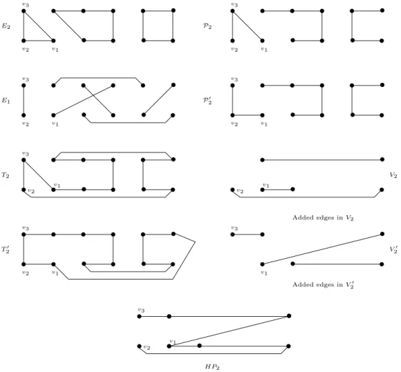
Now, we describe our method. It uses the fact that we assume the existence of a triangle Cp = {v1, v2, v3} in E2in order to apply two times the previous construction, thus producing 4 collections of paths P1, P2,P1′,P2′, as follows.
We apply once the construction and get a first couple P1, P2. Then remark that, at each iteration in the construction, we can choose the vertex v incident to the two edges candidate to move from E2 to E1. Then, wlog., assume that when applying the first construction the edge [v1, v2] has moved from Cp ∈ E2 to E1. To get P1′,P2′, we apply exactly the same construction as previously, except for the last cycle. For Cp, we choose to move one of the two edges [v1, v3] or [v2, v3] incident to v3 (instead of [v1, v2]). Wlog, assume that it is [v1, v3]; using arguments of the proof of Lemma 2.1, we obtain two other collections of paths P1′ (containing E1) and P2′ satisfying properties (i), (ii) and (iii).
Moreover, if V′
i denotes the endpoints of Pi′ for i = 1, 2, then we can observe that v3 ∈ V1, v2 ∈ V1′ and V1\ {v3} = V1′\ {v2}. Thus, it is possible to complete P1into a tour T1
and P1′ into a tour T1′ such that the added edges form an hamiltonian path HP1 on vertices V1∪ {v2} and with endpoints v2, v3.
Similarly, we have v2 ∈ V2, v3 ∈ V2′ and V2\ {v2} = V2′\ {v3}. Thus, we can also add some edges to P2 (resp., P2′) in order to obtain a tour T2 (resp., T2′) in such a way that the added edges form an hamiltonian path HP2 on vertices V2∪ {v3} and with endpoints v2, v3. An illustration of this construction is given in Figure 2. For completeness, let us also give a formal proof of this claim for HP2. Let V2 = {ai, bi : i = 1, . . . p} be the endpoints of the paths of P2, where [ai, bi] is the edge that has moved from E2 to E1 at iteration i. In particular, we have ap = v1 and bp = v2. Similarly, let V2′ = {a′i, b′i : i = 1, . . . p} be the endpoints of the paths of P′
2 with a′p = v1 = ap, b′p = v3 and a′i = ai, b′i = bi for i = 1, . . . , p − 1. The two tours T2 and T2′ depend on the parity of p and can be described as follow.
• Assume first that p is odd. We build T2 = P2 ∪ {[ai, bi+1] : i = 1, . . . , p} and T2′ = P2′ ∪ {[b′
i, a′i+1] : i = 1, . . . , p}, with bp+1 = b1 and ap+1′ = a′1. Since ap = a′p, bp = v2, b′p = v3, and a′i = ai, b′i = bi for i = 1, . . . , p − 1, we deduce that the added edges HP2 = {[ai, bi+1], [b′i, a′i+1] : i = 1, . . . , p} form an hamiltonian path from b′p to bp described by the sequence HP2 = (b′p, a1, b2, . . . , ap, b1, a2, b3, . . . , bp).
• Now, if p is even, then we only modify T′
2 and define T2′ = P2′ ∪ {[b′i, a′i+1] : i = 1, . . . , p − 1} ∪ {[a′
p, a′1], [b′p, b′p−1]}. As previously, one can easily check that the added edges HP2 = {[ai, bi+1] : i = 1, . . . , p} ∪ {[b′i, a′i+1] : i = 1, . . . , p − 1} ∪ {[a′
1, a′p], [b′p, b′1]} form an hamiltonian path from b′1 to b1 described by the sequence HP2= (b′p, b1, a2, b3, . . . , ap, a1, b2, a3, . . . , ap−1, bp).
In conclusion, we get 4 tours T1, T1′, T2 and T2′. By taking the solution of maximum weight with cost apx(I), we obtain:
4apx(I) ≥ 2 X
i=1
(w(Ti) + w(Ti′)) = 2(w(E1) + w(E2)) + (w(HP1) + w(HP2)) (1)
On the one hand, we have w(E2) ≥ opt(I) and w(E1) ≥ opt(I)/2, and on the other hand since HP1 ∪ HP2 is a tour on K2n, we get w(HP1) + w(HP2) ≥ wor(I). Plugging these inequalities with inequality (1), we deduce:
apx(I) ≥ 3
4opt(I) + 1
4wor(I) (2)
Case 2: For all j ∈ {1, . . . , p} we have |Cj| ≥ 4. In this case, we extend the method proposed in [20, 25]. We study 2 subcases depending on the parity of p.
Case 2.1: If p is odd. Obviously, we can assume p > 1. For each cycle Ciof the 2 matching E2 = {C1, . . . , Cp}, we consider 4 consecutive edges Ai = {[ai, bi], [bi, ci], [ci, di], [di, fi]} 1(with eventually f
i= ai if |Cj| = 4), and we produce 4 solutions by starting from E2: the first solution Ta deletes the edge [ai, bi] for each cycle Ci with i = 1, . . . , p, and for each
Added edges in V′ 2 v3 H P2 v2 v1 v1 v2 v1 v2 v3 v3 v3 v1 v3 v2 v2 v1 v1 v2 v1 v3 V′ 2 V2 v3 v2 v1 v3 v2 v1 P2 P′ 2 T2 T′ 2 E1 E2 Added edges in V2
Figure 2: The construction of tours T2 and T2′ and the hamiltonian path HP2.
i ∈ {1, . . . , p − 1} adds the edge [ai, ai+1] if i is odd, adds the edge [bi, bi+1] if i is even and finally adds the edge [ap, b1]. The 3 other solutions Tb, Tc and Td are described similarly by deleting edges [bi, ci], [ci, di] and [di, fi] respectively. In particular, for the last solution Td, we have added for i ∈ {1, . . . , p − 1} the edges [di, di+1] if i is odd, [fi, fi+1] if i is even and finally edge [dp, f1].
In the multigraph of these 4 solutions, that is (V, Ta+ Tb + Tc + Td), each edge e of A = ∪pi=1Ai appears exactly 3 times whereas the other edges of E2appears exactly 4 times. On the other hand, the edges of B = (Ta∪ Tb∪ Tc∪ Td) − E2 appears one time.
Thus, by considering the best of the 4 solutions we produced, we get: 4apx(I) ≥ 3w(A) + 4w(E2− A) + w(B) = 3w(E2) + w(B + E2− A) ≥ 3opt(I) + w(B + E2− A).
Now, remark that B +E2−A is a tour of I. Indeed, E2−A contains paths (fi, gi, . . . , ai) for each i = 1, . . . , p. In B, we get a path P = (ap, b1, b2, . . . bp, c1, . . . , cp, d1, . . . , dp, f1), and edges [ai, ai+1] (i odd) or [fi, fi+1] (i even). These edges and the paths of E2−A create a path from f1 to ap, which constitutes together with P a tour. Hence, w(B + E2− A) ≥ wor(I). We get:
apx(I) ≥ 3
4opt(I) + 1
Case 2.2: If p is even, then the previous construction does not produce a tour. We adapt it as follows. As previously, we consider 4 consecutive edges Ai = {[ai, bi], [bi, ci], [ci, di], [di, fi]} in cycle Ci of the 2-matching E2, except for the last cycle Cpwhere we replaced edge [dp, fp] by [zp, ap] with zp is the other neighbor of ap in Cp (eventually, zp = dp if |Cp| = 4). Thus, Ap = {[zp, ap], [ap, bp], [bp, cp], [cp, dp]}.
Moreover, for C2, we do not choose consecutive vertices a2, b2, c2, d2, f2 at random. We choose them such that:
w([a1, b2]) + w([a2, b1]) ≤ w([a1, a2]) + w([b1, b2]) (4) Actually, this is always possible since otherwise for all e = [x, y] ∈ C2 we would get w([a1, y]) + w([a2, x]) < w([a1, x]) + w([b1, y]) (here, we assume that each edge e = [x, y] is considered as a directed edge where the orientation is given when one walks around C2). Summing up the previous inequality for each edge e ∈ C2, we obtain the inequality P
v∈V(C2)(w([a1, v]) + w([b1, v])) >
P
v∈V(C2)(w([a1, v]) + w([b1, v])), contradiction.
Then, we produce 4 tours Ta, Tb, Tc and Td as follows: first, Ta deletes from E2 edges [ai, bi+1] if i < p and [zp, ap]; then, solution Ta adds edges [ai, ai+1] if i < p is odd, adds the edge [bi, bi+1] if i < p is even and finally adds the edge [zp, b1]. The other tours Tb, Tc and Td are constructed similarly. In particular, Td deletes edges [di, fi] if i < p and [zp, ap], adds for i ∈ {1, . . . , p − 1} edges [di, di+1] if i is odd, [fi, fi+1] if i is even and edge [cp, f1]. As previously, in the multigraph (V, Ta+ Tb + Tc + Td), each edge e of A = ∪pi=1Ai appears exactly 3 times whereas the other edges of E2 appears exactly 4 times. On the other hand, the edges of B = (Ta∪Tb∪Tc∪Td)−E2 appears one time. Thus, by considering the best of these 4 solutions, we get:
4apx(I) ≥ 3w(A) + 4w(E2− A) + w(B) = 3w(E2) + w(B + E2− A) (5) However, now B + E2 − A is not a tour of I, but a 2-matching constituted by two cycles. The first one is (b1, b2, . . . , bp, d1, . . . , dp, g1, . . . , gp, b1), constituted of edges in B ; the second one is constituted by the path (ap, c1, . . . , cp, f1) of B, the paths (fi, gi, . . . , zi, ai) of E2− A, and edges [ai, ai+1] (i odd) or [fi, fi+1] (i even).
But using inequality (4), one can flip edges [a1, a2], [b1, b2] by edges [a1, b2], [a2, b1] with-out increasing the global weight and one obtain a tour T such that wor(I) ≤ w(T ) ≤ w(B + E2− A). In conclusion, using this inequality and inequality (5), we obtain:
apx(I) ≥ 3
4opt(I) + 1
4wor(I) (6)
Combining the results obtained in cases 1 (equation (2)) and 2 (equation (6)), we obtain the following result.
Theorem 2.2 When the number of vertices is even, symmetric TSP is 3/4-differential approximable.
3
General case
In the previous section, we dealt with even instances. Here, we show that one can solve symmetric TSP also on odd instances within an asymptotic differential ratio of 3/4.
Theorem 3.1 In the general case, symmetric TSP can be differential approximated with ratio 3/4 − O(1/n).
Proof: From the discussion above, we have to deal with instances the number of vertices of which is odd. In this case, we find a (3/4 − O(1/n))-approximate solution using the previous result on even instances. Let n odd, I = (Kn, w) an instance of symmetric TSP and denote V = {v1, . . . , vn} the set of vertices.
We find an approximate solution as follows: for each i ∈ {1, . . . , n}, we consider the sub-instance Ii on the subgraph induced by V \ {vi}. On this instance, we apply our approximation method given above and get a tour Ti. Then, we insert vi in the best position in Ti, thus producing a tour Ti′ on I. Finally, we take the best tour T among these n tours T′
i, i.e. apx(I) = w(T ) = maxi=1,...,nw(Ti′).
Note that, when inserting vertex vi in Ti between two vertices vj and vk (consecutive in Ti), we get a tour of value w(Ti) + w([vj, vi]) + w([vi, vk]) − w([vj, vk]). Since we take the best of these nodes, by considering the n − 1 possible insertions, we get:
(n − 1)w(Ti′) ≥ (n − 1)w(Ti) + 2 X k,k6=i w([vi, vk]) − w(Ti) ≥ (n − 2)w(Ti) + 2 X k,k6=i w([vi, vk])
Since we take the best tour among the T′
i’s, we get: n(n − 1)apx(I) ≥ (n − 2) n X i=1 w(Ti) + 2S (7) where S =Pn i=1 P
k,k6=iw([vi, vk]) is twice the total weight of all edges in the graph. Similarly, by inserting vi in any position in a worst tour on Ii, we get a tour on I. The worst solution on I is of course worse than each of these solutions, i.e.:
(n − 1)wor(I) ≤ (n − 1)wor(Ii) + 2 X k,k6=i w([vi, vk]) − wor(Ii) ≤ (n − 2)wor(Ii) + 2 X k,k6=i w([vi, vk]) Hence: n(n − 1)wor(I) ≤ (n − 2) n X i=1 wor(Ii) + 2S (8)
Finally, consider an optimum solution (v∗1, v∗2, . . . , v∗n) on I. By deleting vi∗ in this tour, we get a tour on Iithe value of which is opt(I)−w([vi∗, vi−1∗ ])−w([vi∗, vi+1∗ ])+w([v∗i−1, vi+1∗ ]) ≤ opt(Ii). By considering each of the possible deletion, we get (obviously v0∗ means vn∗ and vn+1∗ means v1∗): n × opt(I) − 2 n X i=1 w([v∗i, v∗i+1]) + n X i=1 w([vi−1∗ , v∗i+1]) ≤ n X i=1 opt(Ii) Since n is odd,Pn
i=1w([v∗i−1, vi+1∗ ]) is the value of a tour, hence at least wor(I). Then:
(n − 2) × opt(I) + wor(I) ≤ n X
i=1
Now, using equations (7), (8), (9) and the fact that w(Ti) ≥ (3opt(Ii) + wor(Ii))/4, we get: 4n(n − 1)apx(I) ≥ 3(n − 2) n X i=1 opt(Ii) + (n − 2) n X i=1 wor(Ii) + 8S
≥ 3(n − 2)2opt(I) + 3(n − 2)wor(I) + n(n − 1)wor(I) + 6S Finally, recall that S is twice the total weight of the n(n − 1)/2 edges of the graph. But by symmetry, the medium value of all the tours on the graph is equal to n times the medium value of the edges, i.e. n × S/(n(n − 1)). This medium value of the tours is of course greater than the worst value. Hence, wor(I) ≤ S/(n − 1). This leads to:
4(n2− n)apx(I) ≥ 3(n2− 4n + 4)opt(I) +¡n2+ 8n − 12¢ wor(I)
This is apx(I) = (3/4 − α(n))opt(I) + (3/4 + α(n))wor(I), where α(n) = (9n − 12)/(4n2− 4n) = O(1/n) (remark that 4(n2− n) = 3(n2− 4n + 4) + (n2+ 8n − 12)).
Let us remark that Theorem 3.1 also holds for any ρ-differential approximation of sym-metric TSP: any ρ-differential approximation algorithm of symsym-metric TSP on even instances can be polynomially converted in a ρ(1−α(n))-differential approximation of symmetric TSP (working on any instance) where we recall that α(n) = (9n − 12)/(4n2− 4n) = O(1/n).
An interesting open question is to know whether one can improve the differential ratio of 1/2 for asymmetric TSP given in [20] using similar ideas.
References
[1] S. Arora. Polynomial time approximation scheme for Euclidean TSP and other geo-metric problems. In Proceedings of the 37th Ann. IEEE Symposium on Foundations of Computer Science, pages 2–11. IEEE Computer Society, 1996.
[2] G. Ausiello, A. D’Atri, and M. Protasi. Structure preserving reductions among convex optimization problems. J. Comput. Syst. Sci., 21(1):136–153, 1980.
[3] G. Ausiello, A. Marchetti-Spaccamela, and M. Protasi. Toward a unified approach for the classification of NP-complete optimization problems. Theor. Comput. Sci., 12:83–96, 1980.
[4] G. Ausiello and V. Th. Paschos. Differential ratio approximation, chapter 16 in Hand-book of Approximation Algorithms and Metaheuristics, Teofilo F. Gonzalez (Ed). Tay-lor and Francis, 2007.
[5] C. Bazgan, R. Hassin, and J. Monnot. Approximation algorithms for some vehicle routing problems. Discrete Applied Mathematics, 146(1):27–42, 2005.
[6] C. Bazgan, J. Monnot, V. T. Paschos, and F. Serri`ere. On the differential approxima-tion of min set cover. Theor. Comput. Sci., 332(1-3):497–513, 2005.
[7] C. Bazgan and V. Th. Paschos. Differential approximation for optimal satisfiability and related problems. European Journal of Operational Research, 147(2):397–404, 2003. [8] Z.-Z. Chen, Y. Okamoto, and L. Wang. Improved deterministic approximation
[9] N. Christofides. Worst-case analysis of a new heuristic for the traveling salesman problem. Technical report 338, Grad. School of Industrial Administration, CMU, 1976. [10] M. Demange, P. Grisoni, and V. T. Paschos. Approximation results for the minimum
graph coloring problem. Inf. Process. Lett., 50(1), 1994.
[11] M. Demange, P. Grisoni, and V. Th.. Paschos. Differential approximation algorithms for some combinatorial optimization problems. Theoretical Computer Science, 209(1-2):107–122, 1998.
[12] M. Demange, J. Monnot, and V. Th.. Paschos. Bridging gap between standard and differential polynomial approximation : the case of bin-packing. Applied Mathematics Letters, 12:127–133, 1999.
[13] M. Demange, J. Monnot, and V. Th.. Paschos. Maximizing the number of unused bins. Foundations of Computing and Decision Sciences, 26(2):169–186, 2001.
[14] M. Demange and V. Th.. Paschos. On an approximation measure founded on the links between optimization and polynomial approximation theory. Theoretical Computer Science, 158(1-2):117–141, 1996.
[15] R. Duh and M. F¨urer. Approximation of k-set cover by semi-local optimization. In STOC, pages 256–264, 1997.
[16] B. Escoffier and V. Th.. Paschos. Differential approximation of MIN SAT, MAX SAT and related problems. European Journal of Operational Research, 181(2):620–633, 2007.
[17] M. M. Halld´orsson. Approximating discrete collections via local improvements. In Proceedings of the Symposium on Discrete Algorithms, pages 160–169, 1995.
[18] M. M. Halld´orsson and E. Losievskaja. Independent sets in bounded-degree hyper-graphs (to appear). In Proceedings of the Algorithms and Data Structures, 2007. [19] D. Hartvigsen. Extension of Matching Theory. PhD thesis, Carnegie-Mellon University,
1984.
[20] R. Hassin and S. Khuller. z-approximations. J. of Algorithms, 41(2):429–442, 2001. [21] R. Hassin and J. Monnot. The maximum saving partition problem. Operations
Re-search Letters, 33:242–248, 2005.
[22] R. Hassin and S. Rubinstein. Better approximations for max TSP. Inf. Process. Lett., 75(4):181–186, 2000.
[23] R. Hassin and S. Rubinstein. A 7/8-approximation algorithm for metric Max TSP. Inf. Process. Lett., 81(5):247–251, 2002.
[24] R. M.. Karp. Reducibility among combinatorial problems. In R. E.. Miller and J. W.. Thatcher, editors, Complexity of Computer Computations, pages 85–103. Plenum Press, 1972.
[25] J. Monnot. Differential approximation results for the traveling salesman and related problems. Inf. Process. Lett., 82(5):229–235, 2002.
[26] J. Monnot, V. T. Paschos, and S. Toulouse. Approximation algorithms for the traveling salesman problem. Mathematical Models of Operations Research, 56:387–405, 2002. [27] J. Monnot, V. T. Paschos, and S. Toulouse. Differential approximation results for
traveling salesman problem with distance 1 and 2. European Journal of Operational Research, 145(3):537–548, 2003.
[28] C. H. Papadimitriou and M. Yannakakis. The traveling salesman problem with dis-tances one and two. Mathematics of Operations Research, 18:1–11, 1993.
[29] A. I. Serdyukov. An algorithm with an estimate for the traveling salesman problem of the maximum. Upravlyaemye Sistemy (in Russian), 25:80–86, 1984.
[30] A. I.. Serdyukov. An asymptotically exact algorith for the traveling salesman problem for a maximum in euclidian space. Uppravlyaemye Sistemy (in Russian), 27:79–87, 1987.
[31] S. A. Vavasis. Approximation algorithms for indefinite quadratic programming. Math. Program., 57:279–311, 1992.