HAL Id: hal-00566168
https://hal.archives-ouvertes.fr/hal-00566168v2
Preprint submitted on 13 Jul 2012
HAL is a multi-disciplinary open access archive for the deposit and dissemination of sci-entific research documents, whether they are pub-lished or not. The documents may come from teaching and research institutions in France or abroad, or from public or private research centers.
L’archive ouverte pluridisciplinaire HAL, est destinée au dépôt et à la diffusion de documents scientifiques de niveau recherche, publiés ou non, émanant des établissements d’enseignement et de recherche français ou étrangers, des laboratoires publics ou privés.
The quality effect of intrafirm bargaining with
endogenous worker flows
Tristan-Pierre Maury, Fabien Tripier
To cite this version:
Tristan-Pierre Maury, Fabien Tripier. The quality effect of intrafirm bargaining with endogenous worker flows. 2011. �hal-00566168v2�
The quality e¤ect of intra…rm bargaining with endogenous worker ‡ows
Tristan-Pierre Mauryy Fabien Tripierz
July 13, 2012
Abstract
This paper proposes a new explanation of the job quality issue in search and matching models, which is not based on market externalities but on strategic interactions within …rms through the intra…rm bar-gaining process. We develop a matching and intra…rm barbar-gaining model in which large …rms hire workers on a frictional labour market and decide to destroy low productivity job-worker matches. The coexistence of entry and exit ‡ows of workers in a large …rm gives rise to a speci…c interaction between the …ring decision and the intra…rm bargaining process on wages, which causes ine¢ cient decisions to be made on hiring and …ring. The sources of ine¢ ciency in this economy are (i) the well-known quantitative e¤ect of intra…rm bargaining, namely the excessive size of the …rms concerned, and (ii) a new quality e¤ect, namely the poor quality of the job-worker matches selected by …rms.
Keywords: Matching; Intra…rm Bargaining; Worker Flows. JEL Classi…cation: J3; J6.
We thank Giuseppe Bertola, Pierre Cahuc, William Hawkins, Philipp Kircher and the participants of the inaugural confer-ence of the European Search and Matching (SaM) network at the University of Bristol (2011). The usual disclaimers apply.
yEDHEC Business School, Economic Research Centre, Email: [email protected] zUniversity of Nantes, Lemna, Email: [email protected]
1
Introduction
The quality of jobs is a highly debated topic in labor economics from both empirical and theoretical
per-spectives. The empirical debate started in the eighties, when some economists, as Bluestone and Harrison
(1988), have warned of the rising number of low-quality jobs; see Goos and Manning (2007) for an recent
as-sessment of this view. The theoretical debate has focused on the ability of the competitive market to provide
the e¢ cient quality of jobs. The seminal contributions of Stevens (1994), Redding (1996) and Acemoglu
(2001) showed that the quality of jobs is generally ine¢ cient with labor market search frictions because
of market externalities.1 In this paper, we provide a new explanation of the bias toward low-quality jobs,
which is not based on market externalities but on the intra…rm bargaining mechanism described by Stole
and Zwiebel (1996ab).2 The bias toward low-quality jobs is the outcome of the strategic interactions within
…rms between the bargaining process on wages with workers and the selection of the quality of worker-job
matches by …rms. This result is obtained by extending the matching and intra…rm bargaining literature
initiated by Smith (1999), Cahuc and Wasmer (2002) and Cahuc et al. (2008) to the case of endogenous
workers ‡ows of entry and exit in …rms.3
The empirical literature on labour market ‡ows has highlighted the importance of workers ‡ows and
of its distinction with job ‡ows. Job ‡ows are associated with the net variation in the mass of jobs at
the establishment level: job destruction only occurs in contracting establishments, in which the total mass
of jobs falls, while job creation only occurs in expanding establishments, in which the total mass rises,
1
Stevens (1994) considers externalities between …rms in the provision of on-the-job training and Redding (1996) pecuniary externalities between investments in human capital (by workers) and in R&D (by …rms). In Acemoglu (2001), pecuniary externalities are the result of an hold-up phenomena associated with the choice of capital by …rms.
2Stole and Zwiebel (1996ab) develop a general setup to study the joint decisions on wages and on the organization of …rms and describe the ine¢ ciencies induced by the strategic interactions between these decisions.
3The job destruction process is exogenous in Smith (1999), Cahuc and Wasmer (2002) and Cahuc et al. (2008). The …rms’ training e¤ort in matching and intra…rm bargaining models is studied by Tripier (2011), but still with exogenous job destruction. Matching and intra…rm bargaining models with endogenous …rms dynamics are presented and discussed below.
see Davis and Haltiwanger (1990). Job creation and job destruction cannot simultaneously occur within
establishments, and only establishments heterogeneity can permit the reallocation of jobs. The picture is
somewhat di¤erent for worker ‡ows because the entry and exit of workers may take place simultaneously
in …rms. Among others, Burgess et al. (2000) demonstrated that worker ‡ows largely exceed job ‡ows,
and that regardless of its size or the growth in its number of employees, entry and exit worker ‡ows occur
simultaneously in most establishments.4 We develop a matching and bargaining model consistent with this
speci…city of worker ‡ows (i.e., that entry and exit ‡ows occur simultaneously within …rms) and use this
model to assess the potential ine¢ ciencies in the quantity and the quality of the job-worker matches in the
labour market.
In order to study worker ‡ows within large …rms, we cannot use the traditional matching and
bar-gaining model of the labour market developed by Diamond (1982), Pissarides (2000), and Mortensen and
Pissarides (1994), in which …rms are small and composed of one single job.5 We must instead consider the
decisions of large …rms composed of heterogeneous job-worker matches. Jobs and workers are homogeneous,
but when they are matched, the e¤ective productivity of each job-worker pair is subject to idiosyncratic
productivity shocks. It is widely-known that considering large …rms with a non trivial production function
(i.e., a concave technology) has strong normative implications. While there exists a condition of e¢ cient
bargaining when …rms are small6, the wage negotiation is generally ine¢ cient in large …rms. It proceeds from
the strategic interactions between the …rm’s decisions on the organisational design of production and the
processes of wage bargaining with workers originally described by Stole and Zwiebel (1996a,b) and known
as intra…rm bargaining. One of their key …ndings was that intra…rm bargaining causes …rms to overemploy
workers in order to reduce their individual marginal productivities, thereby reducing the individual wage
4
These facts have been updated and con…rmed for the US economy by Davis et al. (2006) who combine the most recent datasets including the Job Openings and Labor Turnover Survey.
5
Kiyotaki and Lagos (2007) and Burgess and Turon (2010) make the distinction between job ‡ows and worker ‡ows in matching models with small …rms by assuming that a job can survive after a separation with a worker and be …lled with another worker.
bargained with each worker. Smith (1999), Cahuc and Wasmer (2001), and Cahuc et al. (2008) all studied
the e¤ects of intra…rm bargaining on hiring in the matching model.7 Our aim herein is to extend this
liter-ature to the case of endogenous worker reallocation driven by hiring and …ring. Because the …ring decision
endogenises the average quality of the job-worker matches in …rms, we can identify a new qualitative e¤ect
of intra…rm bargaining in addition to the traditional quantitative e¤ect associated with the size of …rms.
The novelty of our approach lies in the decision to address the issue of intra…rm bargaining in a setup
where …rms simultaneously hire and …re workers. This is in contrast with the literature that has considered
the issue of intra…rm bargaining in models of heterogeneous …rms that either create or destroy jobs in the
tradition of Bertola and Caballero (1994), such as for example, Bertola and Garibaldi (2001), Koeniger and
Prat (2007), Fujita and Nakajima (2009), Cosar et al. (2010), and Elsby and Michaels (2010). In such
models, contracting …rms destroy jobs when hit by an adverse idiosyncratic shock that causes a drop in
the demand of labour. An important property of this type of model is that workers in contracting …rms
are unable to extract a positive rent from the Nash bargaining program on wages because the marginal
value of a job is zero or negative for the …rm. The wage is consequently set at the worker’s reservation
level that makes its utility equal to that of an unemployed worker. Therefore, wages in contracting …rms
are independent of the decisions of …rms and there is no room for strategic interactions between the …ring
decision and wage bargaining.
For worker ‡ows, because …rms simultaneously hire and …re workers, our setup allows new interactions
to take place between the …ring decision and wage bargaining. Existing matching models with large …rms
that simultaneously hire and …re workers8 are not suitable for our purposes because they generally assume a
trivial production technology, with a constant marginal productivity of labour, which makes the individual
7
The strategic interaction between the …rm’s decision on job creation and the wage bargaining process leads …rms to post an excessive number of vacancies or equivalently to overhire workers.
8
See in particular Merz (1999), Krause and Lubik (2007), Krause et al. (2008), and Faia et al. (2010). In Faberman and Nagypal (2008), the recruitment technology is non-linear (the marginal cost of creation of positions is increasing), but the production technology is linear with a constant marginal productivity of labor.
wage independent of the …rm’s decisions and as a result removes the strategic interactions from the model.
The only exception is Helpman et al. (2010) who studied the consequences of globalisation in a model
where heterogeneous …rms screen workers.9 We depart from several assumptions of Helpman et al. (2010).
First, while we assume perfect competition on the goods market, they consider imperfect competition, hence
intra…rm bargaining is the only source of ine¢ ciency in our setup. Second, we solve a dynamic rather than
a static labour market search model. Third, we consider idiosyncratic productivity of matches at the origin
of …ring instead of the screening technology introduced by them. Fourth, we model explicitly the utility
of unemployed workers, which they normalize to zero. This last point matters because at equilibrium, the
labour market tightness a¤ects wages through the endogenous value of unemployed worker utility.
In our model, we have brought together several di¤erent strands of the literature on matching and
bargaining models. The process of hiring is modelled as in the standard matching model of the labour
market; e.g., Pissarides (2000). Firms post costly vacancies on the labour market and unemployed workers
search passively for a job. An aggregate matching function determines the ‡ow of new hirings according
to the masses of vacancies and unemployed workers. The worker-job matches destruction process is taken
from den Haan et al. (2000). The productivity of matches is heterogeneous due to the presence of non
persistent idiosyncratic shocks.10 The distribution of productivity is the same for newly created matches
and for existing ones. If the match productivity is too low, the worker is …red by the …rm, corresponding
to the endogenous …ring carried out by …rms. Domestic production for unemployed workers ensures that
temporary layo¤ are not preferred to permanent layo¤. In addition, there is an exogenous …ring rate in …rms
that is independent of the match productivity. This structure of shocks was considered by den Haan et al.
9Fujita and Nakajima (2009) develop a business cycle model with both worker ‡ows and job ‡ows, but since separations are exogenous there is no room for the strategic interactions between the …ring decision and wage bargaining considered in this paper.
1 0Considering persistent idiosyncratic shocks would clearly be a more realistic assumption, but that would complicate the analytics of the model making the identi…cation and the interpretation of the strategic interpretation between …ring and wage bargaining more di¢ cult .
(2000) in a model applied to small …rms. We follow the approach of Krause and Lubik (2007), who applied
the same structure of shocks for large …rms, but contrary to these authors, we consider a non-constant
marginal productivity of labour. The concavity of the production technology gives rise to the intra…rm
bargaining issue. The process of bargaining on wages is solved using the solution proposed by Cahuc et al.
(2008) for matching and intra…rm bargaining models. As in Cahuc et al. (2008), there is no …rm entry.11
We show that intra…rm bargaining induces ine¢ cient hiring and …ring rules in the economy. The
individual wage solution of the intra…rm bargaining process depends on two variables that are decided by
the …rm, namely its quantity of matches and its reservation productivity. In the intra…rm bargaining setup,
the …rm tries to increase its pro…ts by reducing workers’productivity in order to push down the bargained
wages. In our setup, the …rm has two means of reaching this aim: it can either increase the quantity of
matches or decrease their average quality. The former is common in the intra…rm bargaining literature,
whereas the second is new and speci…c to our setup of workers ‡ows. To lower the average wage, the
representative …rm seeks to increase its production by posting a number of vacancies that is too high (as
in other models of intra…rm bargaining and matching) and by choosing a level of reservation productivity
that is too low (this e¤ect is speci…c to our setup). We use numerical simulations to quantify the e¤ects
of intra…rm bargaining. For our benchmark calibration, intra…rm bargaining induces an excess supply of
vacancies and an insu¢ cient quality of matches. This result is in the line with the classical overemployment
result of Stole and Zwiebel (1996a,b). Our model shows that with endogenous …ring, overemployment is the
outcome of an excessive supply of vacancies and a …ring rate that is too low. The source of ine¢ ciency in
this economy is not only the excessive size of …rms, but also the poor quality of the jobs selected by them.
The remainder of our article is organised as follows. We describe our model in section 2 and in section
3, we show the resolution of the intra…rm bargaining process on wages, and give a formal de…nition of the
equilibrium and its normative properties. In section 4, we provide some brief conclusions.
1 1
2
The Model
2.1 Hiring, Firing, and Production
In our model, …rms are composed of an endogenous number of job-worker matches, which are subject to
idiosyncratic productivity shocks that are denoted a. At the beginning of each period, existing and newly
formed matches draw a value for a from the cumulative distribution function G ( ), whose density function
is denoted g (:). The …rm i chooses its reservation value for idiosyncratic productivity ait: all matches below
this value are destroyed. The endogenous …ring rate is it= G (ait) and the total separation rate is
it= + (1 ) G (ait) (1)
where is the exogenous …ring rate. The survival rate for both exogenous and endogenous separation
processes is (1 it) :
The aggregate matching function is m (ut; vt) = mutv 1
t with vt=
R1
0 vitdi, which represents the mass
of vacancies posted by all …rms with vitbeing the mass of vacancies posted by the …rm i, and utbeing the mass
of unemployed workers. t = vt=ut is the labour market tightness with q ( t) = m (ut; vt) =vt = m (1= t; 1)
being the probability that a vacancy will be …lled in the next period.
The employment of …rm i is denoted nit, and is the sum of the employment masses over the range of
admissible productivity levels a 2 [ait; 1[
nit =
Z 1
ait
nit(a) da (2)
where nit(a) is the mass of worker-job with productivity a. The derivatives of the output and employment of
…rm i with respect to nit(a) will be used to de…ne the …rm’s contribution to the Nash bargaining process on
wages. During the bargaining process, the …rm can decide to keep or not the marginal worker of productivity
a during the bargaining process. For admissible values of a ait, all bargaining processes lead to wages that
are accepted by both the …rm and the workers and the distribution of nit(a) depends on the endogenous
Indeed, the …rm chooses the lower bound of productivity, ait, and the total number of matches, nit,
through its supply of vacancies, vit, but it does not choose the allocation of workers within the range of
admissible productivity levels [ait; 1[, which is imposed exogenously. For a0 > a00 > ait , the …rm cannot
control the relative sizes of the masses of matches, denoted nit(a0) and nit(a00), even if it would be pro…table
to substitute nit(a00) for nit(a0) : The distribution of matches between [ait; 1[ is non-persistent and is entirely
determined by the exogenous power density function g ( ). The mass of matches of productivity a is given
by
nit(a) =
g (a) 1 G (ait)
nit; for a 2 [ait; 1] (3)
where nit is the aggregate employment and g (a) = [1 G (ait)] the power density function of a for the
(endogenous) range of admissible values for the idiosyncratic productivity.
The evolution of …rm i employment level is
nit+1= 1 it+1 (nit+ vitq ( t)) (4)
in which we assume that each …rm gets a linear proportion vit=vtof the total matches m (ut; vt). Idiosyncratic
productivity shocks are the same for both newly created (vitq ( t)) and existing jobs (nit), and therefore the
same proportion it+1 of jobs is destroyed at the beginning of the period t + 1.
Total output of …rm i at time t is
yit= f (hit) = hit (5)
with 0 < 1 and hit is the amount of e¤ective labor input:
hit= h (nit; ait) = z Z 1 ait anit(a) da = znit Z 1 ait a g (a) 1 G (ait) da (6)
2.2 The Firm’s Program
The discounted sum of the pro…ts of …rm i is
it = 1 X k=t k t z Z 1 aik anik(a) da Z 1 aik e wik nik a0 a0=1 a0=aik; aik; a nik(a) da vik (7) 1 X k=t 1 k+1 t ik+1 (Z 1 aik+1
nik+1(a) da (1 ) [1 G (aik+1)]
Z 1
aik
nik(a) da + vikq ( k)
)
where k;t = (k t)is the discount factor at date k (the reference date is denoted t) and ik+1is the multiplier
of the employment evolution constraint. Two costs are taken into account. First, the recruitment of new
workers is costly and the per-period cost of a vacancy is : Second, the wage for a match of productivity a is
denoted weik( ) and depends on the distribution of employment in the …rm fnik(a0)ga
0=1
a0=aik, the current value
for the reservation productivity faikg ; and the value for the idiosyncratic productivity a. According to the
de…nition of nit(a) given in equation (3), the distribution of employment depends on the two endogenous
variables fnit; aitg and on the speci…cation of the exogenous power density function g ( ). We use this
property and postulate a functional form of individual wage whose arguments are simply fnit; ait; ag rather
than the entire distribution of employment fnit(a0)ga
0=1
a0=aik.
Claim 1 The wage for the value a of the idiosyncratic productivity shock in …rm i is a function of the two
endogenous variables fnit; aitg and writes as follows
e wit nit a0 a0=1 a0=aik; ait; a =weit g (a0) 1 G (ait) nit a0=1 a0=ait ; ait; a ! =weit(nit; ait; a) (8)
This postulate for the individual wage function uses the property (3) and is consistent with the
intra…rm bargaining approach; because the …rm does not decide on the whole distribution of matches, but
only on the mass of matches and the lower bound of the idiosyncratic productivity level, the wage of a
worker with a productivity of a does not depend on the distribution of jobs within the range of productivity
[ait; 1[ for a given …rm size. We will further prove that this speci…cation of the individual wage is consistent
with the outcome of the Nash bargaining process. Therefore, the wage bill is Z 1 aik e wik nik a0 a0=1 a0=aik; aik; a nik(a) da = wit(nit; ait) nit (9)
where wit(nit; ait) is the average wage bill per employee de…ned by wit(nit; ait) = Z 1 ait e wit(nit; ait; a) g (a) 1 G (ait) da (10)
Once again, this expression only depends on the variables nit and ait due to the intra…rm bargaining
assumption.
Finally, the …rm’s problem is to choose its supply of vacancies vit; its reservation value for idiosyncratic
productivity ait, and its employment level nitto maximise the discounted sum of pro…ts de…ned by (7) under
conditions (2), (3), (5), (6), and (10), that is
max vit;nit;ait+1 it = 1 X k=t k t zn ik Z 1 aik a g (a) 1 G (aik) da wik(nik; aik) nik vik (11) 1 X k=t 1 k+1 t
ik+1fnik+1 (1 ) [1 G (aik+1)] (nik+ vikq ( k))g
2.3 The Asset Value of Jobs
To solve the Nash bargaining program, we de…ne the asset value of a job with productivity a for …rm i
Jit(a) = za h (nit; ait) 1 weit(nit; ait; a) (12) Z 1 ait @weit(nit; ait; a0) @nit(a) nit a0 da0 | {z } Intra…rm + " 1 it+1 Z 1 ait+1 Jit+1(a) g (a) 1 G (ait+1) da #
where the …rst term is the marginal productivity of the match of productivity a, see (5)-(6), the second
term is the individual wage, the third term is associated with the "intra…rm e¤ect", and the last term is
the discounted value for the match. With probability 1 it+1 , the match survives and the …rm gets the
average value of future matches.
The third term, associated with the "intra…rm e¤ect", accounts for the impact of the marginal worker
the expressions (8) for the individual wage and (10) for the average wage bill, this term becomes Z 1 ait @weit(nit; ait; ait+1; a0) @nit(a) nit a0 da0= wit1 (nit; ait) nit, 8a 2 [ait; +1[ (13)
that is the product of the marginal impact of employment on the average wage bill and the …rm’s employment
level - see Appendix A.1 for details. It is interesting to note that this expression does not depend on the
idiosyncratic productivity level a. This crucial property of the model follows directly from the postulate on
wage distribution (8). In the Nash bargaining program, we will use the following expression for the asset
value of a job with productivity a for …rm i
Jit(a) = za h (nit; ait) 1 weit(nit; ait; a) w1it(nit; ait) nit (14) + " 1 it+1 Z 1 ait+1 Jit+1(a) g (a) 1 G (ait+1) da # using (12) and (13).
2.4 The Nash Bargaining on Wages
To solve the Nash bargaining process on wages, we …rst de…ne the value of being employed or unemployed
to a worker. The asset value of a match for a worker with productivity a is denoted Wit(a) and de…ned by
Wit(a) = weit(nit; ait; a) + (1 ) [1 G (ait+1)] Z 1 ait+1 Wit+1(a) g (a) 1 G (ait+1) da (15) + [ + (1 ) G (ait+1)] Ut+1
where Ut is the expected return of being unemployed and is de…ned by
Ut= b + tq ( t) 1 t+1 Z 1 at+1 Wt+1(a) g (a) 1 G (at+1) da + 1 tq ( t) 1 t+1 Ut+1 (16)
where b measures home production and the variables in bold show the average values of these variables in
the economy. The wage solution of the bargaining program within …rm i is
Wit(a) Ut=
1 Jit(a) (17)
3
Equilibrium
In this section, we …rst present the wage solution of the intra…rm bargaining process, then we show that it
is consistent with our postulate for the individual wage speci…cation, and then we discuss our …ndings. We
then de…ne the equilibrium and provide some conditions for its e¢ ciency.
3.1 The Wage Solution
3.1.1 The Resolution of the Intra…rm Bargaining Process
The solution of the Nash program (17) is the individual wage function weit( ) that satis…es
e
wit(nit; ait; a) + w1it(nit; ait) nit= (1 ) b + t+ za h (nit; ait) 1 (18)
It should be noted that the implicit functional form of weit deduced from equation (18) is consistent with
our postulate on the wage distribution (8). As is common in intra…rm bargaining models, there is a partial
derivative of the wage function with respect to employment in the equation solution of the bargaining
process. However, in our setup the partial derivative term is the derivative of the average wage wit( ) with
respect to employment, while the interest variable is the individual wage weit( ) : We must therefore …rst
compute the average wage by aggregating the wages de…ned by the equation (18) using the de…nition (10)
of the average wage. The average wage solution of the Nash program (17) solves the partial di¤erential
equation wit(nit; ait) = (1 ) b + t+ @f (h (nit; ait)) @nit wit1 (nit; ait) nit (19) whose solution is wit(nit; ait) = (1 ) b + t+ 1 (1 ) h (nit; ait) nit (20)
This expression for the average wage gives rise to the following equation for the individual wage solution of
the equation (18) e wit(nit; ait; a) = (1 ) b + t+ @f (h (nit; ait)) @nit(a) ( 1) 1 (1 ) @f (h (nit; ait)) @nit (21)
3.1.2 The Impact of Firm’s Decisions on Wages
The average wage is a¤ected by the …rm’s hiring and …ring decisions. The partial derivatives of the average
wage function given by equation (20) with respect to ait and nit are
w1it(nit; ait) = (1 ) 1 (1 ) h (nit; ait) n2it 0 (22) w2it(nit; ait) = 2 1 (1 ) g (ait) 1 G (ait) h (nit; ait) nit 2 41 ait R1 aita g(a) 1 G(ait)da 3 5 > 0 (23)
The negative e¤ect of employment on the average wage measured by w1it( ) corresponds to the classical
"overemployment" result, originally described by Stole and Zwiebel (1996a,b) and afterwards restated in
the context of matching frictions by Smith (1999) and Cahuc et al. (2008). These authors showed that this
e¤ect vanishes if the technology is linear ( = 1). The positive impact of the productivity reservation on
the average wage measured by w2it( ) is the sum of two e¤ects:
wit2 (nit; ait) =
g (ait)
1 G (ait)
[wit(nit; ait) weit(nit; ait; ait)]
| {z }
impact on the average quality
(24) + Z 1 ait e w2it(nit; ait; a) g (a) 1 G (ait) da | {z }
impact on the individual wages
The …rst e¤ect is associated with the "average quality" of matches and exists even if the production function is
linear as in Krause and Lubik (2007).12 Increasing ait improves the average quality of the selected matches
and therefore improves the average wage paid by the …rm: this e¤ect would hold without the intra…rm
bargaining assumption. It is easy to see that this …rst term positively contributes to the impact of the
productivity reservation on the average wage. In our speci…c setup, this …rst e¤ect is augmented by a
second one linked to the impact of the productivity reservation ait on the individual wageweit, which results
directly from the intra…rm bargaining assumption. Using de…nition (21), we deduce that the contribution
1 2
In Krause and Lubik (2007), the linearity of the production function ( = 1) makes the wage bill wit independent of nit, but not of ait.
of this second e¤ect to the average wage is negative: Z 1 ait e w2it(nit; ait; a) g (a) 1 G (ait) da = (1 ) (1 ) 1 (1 ) g (ait) 1 G (ait) h (nit; ait) nit 2 41 ait R1 aita g(a) 1 G(ait)da 3 5 0 (25)
An increase in ait lowers the relative productivity of an a-type worker and consequently reduces the average
wage. Therefore, the intra…rm bargaining assumption considered in an endogenous destruction setup
con-tributes to the mitigation of the positive e¤ect of the productivity reservation on the average wage given by
(24).
3.1.3 Discussion
The individual wage solution of the bargaining process given by equation (21) depends not only on the
…rm’s employment level (as is common in intra…rm bargaining models), but also on the …rm’s decision on
separation. This property makes our setup (based on workers’ reallocation) di¤erent from other intra…rm
bargaining models based on job reallocation such as that of Bertola and Caballero (1994). In these models
of job reallocation, the average wage only depends on the …rm’s level of employment, and not on the …rm’s
productivity threshold under which it destroys jobs or leaves the market.13 Our wage equation is also
di¤erent from that of Helpman et al. (2010), who solved a static model in which the screening ability cuto¤
decided by the …rm simultaneously determines both the quality and the number of workers. Therefore, the
wage equation has only one argument in Helpman et al. (2010), namely the screening ability cuto¤. The
novelty of our approach is that it provides a wage equation solution of the intra…rm bargaining process that
depends both on the …rm’s employment level and its …ring rate. This property will turn out to be decisive
when we will assess the e¢ ciency of the competitive equilibrium, since we can detect two distortions in our
1 3
Bertola and Caballero (1994) give the explicit expression for the wage in contracting …rms that does not depend on …rm’s employment, see equation (19) in their paper, and the wage in expanding …rms that depends on the …rm’s hiring e¤ort, see equation (21) in their paper. For similar wage solutions in models of job reallocation see equation (11) of Bertola and Garibaldi (2001), equation (10) of Elsby and Michaels (2010), equation (9) of Koeniger and Prat (2007), and equation (22) of Fujita and Nakajima (2009).
economy: the intra…rm bargaining assumption distorts both the hiring and …ring decisions.
The distortion of the hiring and …ring decisions could be interpreted in terms of both quantitative
and qualitative e¤ects. The quantitative e¤ect proceeds from the impact of the quantity of matches on
bargained wages and corresponds to the partial derivative (22). Because a greater number of matches
contribute to a lowering of the average wage, …rms are inclined to post too many vacancies and consequently
the equilibrium …rm size is above its optimal level. The interpretation of the quality e¤ect associated with
the reservation productivity is rather less straightforward because it has two opposing consequences. First,
the …rm’s reservation productivity negatively a¤ects the individual bargained wages, as shown by partial
derivative (25), and, this should therefore drive …rms to increase their reservation productivity. Second, the
…rm’s reservation productivity negatively impacts on the e¤ective labour input, de…ned by (6), as shown in
the Appendix A.2, and should therefore drive …rms to decrease their reservation productivity in order to
lower the average wage; see (20). In the following sections we provide a full analysis of these two opposite
e¤ects of the reservation productivity and conclude that the second e¤ect generally dominates the …rst, and
intra…rm bargaining pushes …rms to accept a quality of job-worker matches that is too low.
3.2 The E¢ ciency of the Competitive Equilibrium
Steady-state labour market allocations are determined by two variables: the productivity reservation and
solution of equation (4) is14 n ( ; a) = 1 (1 ) (1 G (a)) (1 ) (1 G (a)) 1 m + 1 1 (n)
with n1( ; a) > 0 and n2( ; a) < 0: The e¤ective labour input h (a; ) is given by equations (6) and (n)
h ( ; a) = z 1 (1 ) (1 G (a)) (1 ) (1 G (a)) 1 m + 1 1Z 1 a a g (a) 1 G (a)da (h)
with h1( ; a) > 0 and h2( ; a) < 0: The steady-state employment level unambiguously increases with
and decreases with a. Hence, h straightforwardly increases with : The overall impact of a on the e¤ective
labour input should be ambiguous because an increase in a lowers the employment rate, but raises the
average quality of matches. We show in the Appendix A.2 that the overall impact is negative. The optimal
and competitive values for (a; ) are now de…ned.
De…nition 1 The optimal values f ; a g, solution of the social planner program described in the Appendix
A.4, solve m ( ) 1 = (1 ) [1 G (a )] h ( ; a ) 1 z h ( ; a ) zn ( ; a ) a (H o) m ( ) 1 + h ( ; a ) 1za = b + (1 ) (Fo)
where the functions h ( ; a) and n ( ; a) are given by Equations (h) and (n). The values f ; a g, solution of
the competitive economy de…ned in Section 2, solve
m ( ) 1 = (1 ) (1 G (a )) (1 ) 1 (1 ) zh ( ; a ) 1 h ( ; a ) zn ( ; a ) a (H ) 1 4
It is computed as follows The steady-state of (4) is
n = (1 ) (n + vq ( )) (26)
The de…nition of the matching process implies vq ( ) = m (1 n) and the de…nition of given by (1) implies (1 ) = (1 ) (1 G (a)). Therefore, (26) becomes
n = (1 ) m 1 (1 ) (1 m ) = m 1 (1 ) 1 + m = 1 1 m h 1 (1 )(1 G(a)) 1 i + 1 = 1 (1 ) (1 G (a)) (1 ) (1 G (a)) 1 m + 1 1
m ( ) 1 +
(1 )
1 (1 ) h ( ; a )
1za = (1 ) b + (F )
see the sections A.3 and A.4 of the Appendix for details of their solution.
The terms on the LHS of the Hiring equations (H ) and (H ) represent the average matching cost
de…ned as the ratio of the per-period search cost to the job matching probability m 1. Equilibrium
hiring equalises this average matching cost to the discounted average value of a …lled job de…ned by the
RHS term of (H ) for competitive …rms, and by the RHS term of (H ) for the social planner. The
dis-count rate is the product of the subjective disdis-count factor and the job survival rate to shocks, i.e.,
(1 ) (1 G (a)). The average marginal productivity of jobs has the same expression for the two
equi-libria, namely zh 1(h= (zn) a), but the social planner considers the share of this productivity rather
than the share (1 ) = [1 (1 )] for competitive …rms. The term [1 (1 )] 1 directly results
from the intra…rm bargaining mechanism.
The terms on the LHS of (F ) and (F ) represent the marginal value of the less productive job-worker
match for competitive …rms and the social planner respectively. Keeping this job makes it possible to save
the average matching cost – the …rst term ( =m) 1 . The second terms on the LHS of (F ) and (F ) are
the shares of the marginal productivity of this match, given by h 1za. As for the hiring equations, these
shares are not identical for the social planner (i.e., ) and for competitive …rms: (1 ) = [1 (1 )].
The RHS term of (F ) and (F ) account for opportunities outside the match, which consist in b the home
production of unemployed workers and = p ( ) =q ( ), the product of the worker matching probability
and the average matching cost. These two terms are weighted by for the social planner and for the
competitive equilibrium.
Proposition 1 The competitive equilibrium is e¢ cient when the Hosios condition holds and the production
technology is linear.
Proof. Equations (H )-(F ) are equivalent to (H )-(F ) if = 1 and the Hosios condition holds
With a linear production technology, the sole distortion in the economy (namely the trading
exter-nality associated with matching function) is e¢ ciently internalised in the labour contract if the bargaining
power of agents correspond to their contribution to the trading activities; see Hosios (1990) and Pissarides
(2000). Hence, the combination of intra…rm bargaining and endogenous …ring decisions generates no further
distortion in the linear case. The competitive equilibrium with a concave production technology is ine¢ cient
even if the Hosios conditions holds.
With a concave production technology, intra…rm bargaining prevents the labour contract from
inter-nalising trading externalities. Intra…rm bargaining creates a distortion in the economy because …rms take
into account the impact of the marginal worker on the total mass of bargained wages with their employees.
Without intra…rm bargaining, the …rm internalises the fraction (1 ) of the marginal productivity of labour
rather than (1 ) = [1 (1 )] with intra…rm bargaining. The term [1 (1 )] 1 corresponds to
the ine¢ ciency induced by intra…rm bargaining and would be equal to 1 without intra…rm bargaining. It
…rst appears in the hiring equation (H ) as in other models of matching and intra…rm bargaining models with
exogenous separation; e.g. Smith (1999) and Cahuc et al. (2008). Firms give a higher value to the marginal
worker with intra…rm bargaining and are therefore more inclined to post vacancies. The originality of our
model is that this term also appears in the …ring equation (F ). The RHS term of (F ) corresponds to the
value of the match with the lowest productivity. Through the term [1 (1 )] 1, intra…rm bargaining
implies that …rms give a higher value to this match than they would do without intra…rm bargaining. Firms
are therefore induced to accept matches with a productivity level below its optimal level. For given values
of h and n; intra…rm bargaining unambiguously promotes an increase in labour market tightness and a fall
in reservation productivity. The full impact is ambiguous, however, because the variables h and n are also
a¤ected by variations of and a. The use of di¤erentiation may help to provide some further understanding
3.3 A Graphical Representation of the Equilibrium
To characterise the equilibrium, we introduce a parameter ' that can take two values. If ' = (1 ), the
so-lution is the outcome of the optimal equilibrium a; = a ; . Otherwise ' = (1 ) = [1 (1 )] ;
and the solution is the outcome of the competitive equilibrium a; = n
a ; o
: For a linear production
technology and under the Hosios condition, the competitive equilibrium is optimal and is at the
intersec-tion of two decreasing curves in the plan (a; ). However, this may not be the case when the producintersec-tion
technology is concave. Full details of the calculations are provided in the Appendix A.5.
The di¤erentiation of the Hiring Curves – either in the optimal (H ) or the competitive case (H ) –
yields m (1 ) + (1 ) ' zT (a) (1 ) h1( ; a) h ( ; a) 2 | {z } >0 d = (1 ) ' z 2 6 6 6 6 6 4 T1(a) h ( ; a) 1 | {z } <0 +T (a) ( 1) | {z } <0 h2( ; a) | {z } <0 | {z } >0 h ( ; a) 2 3 7 7 7 7 7 5 da (27)
where the values of a; and ' vary for the optimal and competitive cases as explained above and assuming
that the Hosios condition still holds. When = 1 the second bracketed term in the RHS of equation (27)
is null and the slopes of the H-curves are negative. For < 1; the sign of d =da depends on the relative
size of the two terms on the RHS, which notably depend on the chosen functional form of g (:), i.e., the
density of productivity shocks. In the numerical section, we will show that under plausible parameterisations
and assuming the log normality of idiosyncratic shocks, the overall sign of the RHS bracket term remains
negative even for low values of . Consequently, the slopes of the H-curves appear to be negative in either
case (optimal or competitive). Moreover, it is easy to see that the higher the value of '; the higher the value
of for a given value of a (see Appendix A.5 for further details). Hence, the intra…rm bargaining assumption
causes the H-curve (H ) to move upwards in the (a; ) plane, therefore contributing to overemployment for
literature).
If we now turn to the impact of intra…rm bargaining on the F-curves, either in the optimal (F ) or
the competitive case (F ), we get
' zh( 1) h2( ; a) h ( ; a) 2a + h ( ; a) 1 i | {z } >0 da = 2 6 6 6 4 1 1 m 1 | {z } <0 + (1 ) ' zh1( ; a) h ( ; a) 2a | {z } >0 3 7 7 7 5d (28)
Once again, we …nd that d =da < 0 when = 1 because the second term on the RHS of equation (28) is null.
However, the role of this term if < 1 makes the slopes of the F-curves slope rather di¢ cult to determine.
As numerical experiments will show, the sign of d =da can turn out to be positive when is low, because
the second term on the RHS dominates the …rst one. Moreover, the sign of d =da may remain ambiguous
(positive for some parts of the curve and negative for others) for intermediate values of : the possibility
of the existence of multiple equilibria can therefore not be excluded. Throughout the numerical exercise,
we will mainly work on cases where the F-curves are monotonic and where an equilibrium exists and is
unique.15 Finally, the overall contribution of the intra…rm bargaining assumption can easily be identi…ed:
for a given value of , the higher the value of '; the lower the value of a. Hence, ' moves the F-curves to
the left in the (a; ) plane. For a given level of market tightness, the intra…rm bargaining then contributes
to a lowering of the average worker productivity. The total (i.e. simultaneously analysing the impact on the
Hiring and Firing Curves) e¤ect of intra…rm bargaining will depend on the respective (and relative) slopes
of the two curves and will be analysed in the numerical experiment below.
3.4 Numerical illustration
In order to illustrate the normative properties of our setup, we now proceed to our numerical simulations.
This will enable us to assess quantitatively the impact of the intra…rm bargaining assumption on the labour
market tightness and the productivity reservation.
3.4.1 Calibration
The model period is one quarter. We set the discount factor = 0:99, making the annual interest rate
close to 4%. Labour income share is set to its standard value, = 0:6. Without any loss of generality, z
is set to 1. For the other calibration constraints, we follow den Haan et al. (2000). We choose an overall
separation rate = 0:1 and set the exogenous …ring rate of = 0:068: Hence, the endogenous separation
rate is G (a) = ( ) = (1 ) = 0:034. As in den Haan et al. (2000), the average matching rate q is set
to 0:7. The unemployment rate u = 1 n is set to 0:12. This rate is higher than its o¢ cial US empirical
counterpart, since it also includes jobseeking out-of-the-labour-force workers (see Cole and Rogerson, 1999).
To ensure the optimality of the ’no intra…rm bargaining’setup, we suppose that workers’and …rms’shares
of the bargaining surplus are similar and equal to 1/2 and impose that (1 ) = = 0:5. Finally, we assume
that the idiosyncratic productivity a is iid lognormally distributed, with mean E [ln (a)] = 0 and standard
error a= 0:1:
Table 1 gives the values of the parameters and steady-state interest variables of the intra…rm bargaining
model deduced from the calibration procedure. The labour market tightness is derived from the dynamic
equation for the employment rate. The endogenous separation rate gives a directly. Finally, the values of
real cost per vacancy , and the home production utility ‡ow b are respectively deduced from the hiring
and …ring equations. The optimal values of the interest variables (here denoted ; a and n ) are deduced
from the no-intra…rm bargaining model through the use of equations (H ), (F ) and (n).
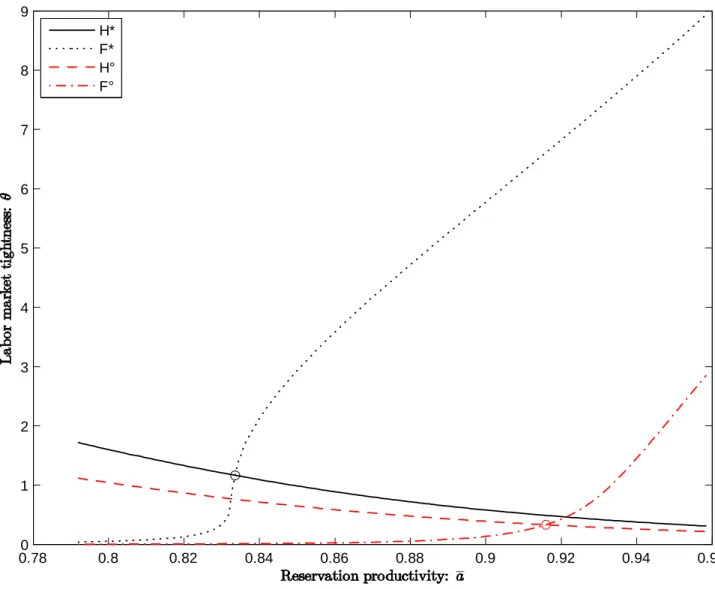
3.4.2 Comparison of the Intra…rm and Optimal Equilibria
Figure 1 provides a steady-state comparison of the hiring (H) and …ring (F ) curves in the intra…rm and
optimal models. For both models, the hiring locus is decreasing and the …ring locus is increasing as in
creation locus represents the hiring one. This proves that for a standard value of the labour income share,
the in‡uence of the second term in the bracket of the RHS of equation (28) dominates that of the …rst
term. This pattern of the locus then ensures the uniqueness of the equilibria for both the competitive and
the optimal models. The labour market tightness is higher in the suboptimal intra…rm setup due to the
analytically detailed upward position of the competitive hiring curve and leftward position of the competitive
…ring curves. Hence, our exercise con…rms the higher labour market tightness e¤ect of intra…rm bargaining
as already detailed in the "exogenous destruction" literature. At the same time, the reservation productivity
appears to be lower in the intra…rm case because of the relative ‡atness of the H-curve (d =da is low in
absolute values). This e¤ect on a is speci…c to our endogenous destruction setup and reinforces the standard
over-tightness result: the overall impact of intra…rm bargaining on the employment rate (see Table 1) is
positive due to the joint overposting of vacancies and the too low …ring rate. The usual "overemployment"
result is worsened here due to the low quality of jobs selected by …rms.
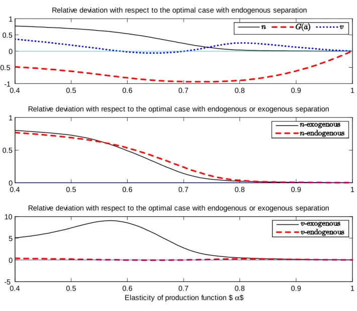
Figure 2 (top panel) shows that, despite the instability of the signs of slope of the F-curve, the
simul-taneous e¤ect of intra…rm bargaining on and a holds a variety of values of . For all values of between
0.4 and 1, the competitive labour market allocations are characterised by excessive hiring, insu¢ cient …ring
and consequently overemployment.16 To put forward the implications of the …ring decision, we also consider
the case of purely exogenous separations (i.e. a = 0). The middle panel of Figure 2 shows that the excessive
size of …rms is quite similar between the two versions of the model (with or without endogenous destruction).
However, as shown by the bottom panel of Figure 2, the excess supply of vacancies is strikingly di¤erent
between the two versions of the model. With endogenous destruction, the excess supply of vacancies is tiny
and, for some values of , the supply of vacancies by …rms is even too small. The excess employment is
mainly the outcome of a too low average separation rate in the economy rather than an excessive supply
of jobs. This picture contrasts with the case of exogenous separation where the large excess of vacancies is
1 6
Note that in some of the intermediate values of considered here (more precisely when is between 0:8 and 0:9), the uniqueness of the equilibrium cannot be guaranteed. The …gure only proposes a comparison based on a range of steady-states calibrated according to the rules described in the calibration subsection.
clearly at the origin of the excessive size of …rms. Therefore, our setup of endogenous worker ‡ows provides
a new view of the excessive …rms’size, which is more the outcome of an insu¢ cient amount of separations
rather than an excessive supply of vacancies.
4
Conclusion
We have herein developed a matching and intra…rm bargaining model of the labour market to study the
e¢ ciency of hiring and …ring by large …rms. The novelty of our approach lies in the consideration of …rms
that simultaneously hire and …re workers as suggested by numerous empirical studies. This approach gives
rise to speci…c interactions between the wage bargaining process and decisions on …ring. We …nd a negative
impact on bargained wages of the productivity threshold under which workers are …red and show how this
impact is included in the …rm’s choice of this threshold. Because of these interactions, the equilibrium is
ine¢ cient and both hiring and …ring decisions are distorted. Hence, our setup complements the standard
"overemployment" result of the intra…rm bargaining literature with exogenous job destruction: we con…rm
that the competitive employment rate is too high in a large …rm setting with endogenous …ring decisions,
but also prove that the average quality of labour matches is too low in this case. Further researches should
5
References
Acemoglu, D. (2001). Good Jobs versus Bad Jobs. Journal of Labor Economics 19(1), 1-21.
Bertola, G., & Caballero, R.J. (1994). Cross-Sectional E¢ ciency and Labour Hoarding in a Matching Model
of Unemployment. Review of Economic Studies 61(3), 435-56.
Bertola, G., & Garibaldi, P. (2001). Wages and the Size of Firms in Dynamic Matching Models. Review of
Economic Dynamics 4(2), 335-368.
Bluestone, B., Harrison, B. (1988) “The Growth of Low-Wage Employment: 1963–1986,” American
Eco-nomic Review 78(2), 124–128.
Burgess, S., & Turon, H. (2010). Worker ‡ows, job ‡ows and unemployment in a matching model. European
Economic Review 54(3), 393-408.
Burgess, S., Lane, J., Stevens, D. (2000). Job Flows, Worker Flows, and Churning. Journal of Labor
Economics 18(3), 473-502.
Cahuc, P., & Wasmer, E. (2001). Does Intra…rm Bargaining Matter in the Large Firm’s Matching Model?
Macroeconomic Dynamics, 5, 742-747.
Cahuc, P., Marque, F., & Wasmer, E. (2008). A Theory of Wages and Labor Demand with Intra-…rm
Bargaining and Matching Frictions. International Economic Review 49(3), 943-972.
Cole, H.L., Rogerson, R. (1999). Can the Mortensen-Pissarides Matching Model Match the Business-Cycle
Facts?, International Economic Review 40(4), 933-59.
Co¸sar, A.K., Guner, N., Tybout, J. (2008). Firm Dynamics, Job Turnover, and Wage Distributions in an
Open Economy. NBER Working Paper No. 16326.
Davis, S.J., Faberman R.J., & Haltiwanger, J.. "The Flow Approach to Labor Markets: New Data Sources
Davis, S.J., Haltiwanger, J. (1990). Gross Job Creation and Destruction: Microeconomic Evidence and
Macroeconomic Implications, NBER Macroeconomics 5,123-186.
den Haan, W.J., Ramey, G., & Watson, J. (2000). Job Destruction and Propagation of Shocks. American
Economic Review 90(3), 482-498.
Diamond, P. A. (1982). Aggregate Demand Management in Search Equilibrium. Journal of Political
Econ-omy 90(5), 881-94.
Elsby, M.W.L., & Michaels, R. (2008). Marginal Jobs, Heterogeneous Firms, and Unemployment Flows.
NBER Working Papers 13777.
Goos, M., Manning, A. (2007) Lousy and Lovely Jobs: the Rising Polarization of Work in Britain. Review
of Economics and Statistics 89(1), 118-133.
Faia, E., Lechthaler, W., & Merkl, C. (2009). Labor Selection, Turnover Costs and Optimal Monetary
Policy, IZA Working papers 4322.
Fujita, S., & Nakajima, M. (2009). Worker ‡ows and job ‡ows: a quantitative investigation. Working
Papers 09-33, Federal Reserve Bank of Philadelphia.
Hamermesh, D.S., Hassink, W. H. J., Van Ours, J.C. (1996). Job Turnover and Labor Turnover: A taxinomy
of Employment Dynamics. Annales d’Economie et de Statistique 41-42, 21-39.
Helpman, E., Itskhoki, O., & Redding, S. (2010). Inequality and Unemployment in a Global Economy.
Econometrica 78(4), 1239-1283.
Hosios, A. (1990). On the E¢ ciency of Matching and Related Models of Search and Unemployment. Review
of Economic Studies, 57(2), 279-298.
Kiyotaki, N., Lagos, R. (2007). A Model of Job and Worker Flows, Journal of Political Economy 115(5),
770-819.
Economic Journal 117(521), 302-332.
Krause, M., & Lubik, T. (2007). Does intra-…rm bargaining matter for business cycle dynamics?. Deutsche
Bank Discussion Paper, Series 1: Economic Studies No 17/2007.
Krause, M.U., Lopez-Salido, D.J., & Lubik, T. A. (2008). Do search frictions matter for in‡ation dynamics?
European Economic Review 52(8), 1464-1479.
Ljungqvist, L. (2002). How Do Layo¤ Costs A¤ect Employment? Economic Journal (2002), 829-853.
Mortensen, D. T., & Pissarides, C.A. (1994). Job Creation and Job Destruction in the Theory of
Unem-ployment. Review of Economic Studies 61(3), 397-415.
Pissarides, C.A. (2000). Equilibrium unemployment theory (Second edition). MIT Press.
Redding, S., (1996). The Low-skill, Low-quality Trap: Strategic Complementarities between Human Capital
and R & D. Economic Journal 106(March), 458-470.
Smith, E. (1999). Search, Concave Production, and Optimal Firm Size. Review of Economic Dynamics,
2(2), 456-471.
Stevens, M. (1994). Labour Contracts and E¢ ciency in on-the-Job Training. Economic Journal 104(March),
408-419.
Stole, L., & Zwiebel, J. (1996a). Intra-…rm Bargaining under Non-binding Contracts. Review of Economic
Studies, 63(3), 375-410.
Stole, L., & Zwiebel, J. (1996b). Organizational Design and Technology Choice under Intra…rm Bargaining.
American Economic Review, 86(1), 195-222.
Tripier, F. (2011). The E¢ ciency of Training and Hiring with Intra…rm Bargaining, Labour Economics,
A
Appendix
A.1 Calculus for the "intra…rm e¤ect"
The term associated with the "intra…rm e¤ect" in the value function (12) is Z 1
ait
@weit(nit; ait; a)
@nit(a)
nit(a) da (A.1)
To get its expression given by (13), we proceed as follows. First, given the de…nition of aggregate employment
(2) we can rewrite this term as
Z 1 ait @weit(nit; ait; a) @nit @nit @nit(a) nit(a) da (A.2)
where @nit=@nit(a) = 1. Second, introducing the expression of nit(a) given by (3) and the de…nition of the
wage bill (8) lead to
Z 1 ait @weit(nit; ait; a) @nit g (a) 1 G (ait) da nit (A.3)
because the functions g (:) and G (:) do not depend on nit, it is equivalent to
@ @nit Z 1 ait e wit(nit; ait; a) g (a) 1 G (ait) da | {z } wit(nit;ait) nit (A.4)
where the term in brackets is the average wage according to de…nition (10). Hence, the …nal expression
given by (13): w1it(nit; ait; ait+1) nit:
A.2 Properties of the function h
The function h ( ; a) is h ( ; a) = zn ( ; a) Z 1 a a g (a) 1 G (a)da (h)
where the steady-state employment level n (a; ) is for the Cobb-Douglas matching function
n ( ; a) = 1 (1 ) (1 G (a)) (1 ) (1 G (a)) 1 m + 1 1 (A.5)
with n1( ; a) > 0 and n2( ; a) < 0: The partial derivatives of h ( ; a) are h1( ; a) = zn1( ; a) Z 1 a a g (a) 1 G (a)da > 0 (A.6) h2( ; a) = z 2 6 6 6 6 6 6 6 6 6 6 6 4 n2( ; a) | {z } "quantity e¤ect"<0 R1 a a g(a) 1 G(a)da +n ( ; a)1 G(a)g(a) Z 1 a a g (a) 1 G (a)da a | {z } "quality e¤ect">0 3 7 7 7 7 7 7 7 7 7 7 7 5 (A.7)
using the de…nition of n (a; ) gives
n2( ; a) = g (a) (1 ) (1 G (a))2 1 m ( ) n ( ; a) 2< 0 (A.8) therefore h2( ; a) = zn ( ; a) g (a) 1 G (a) " 1 n ( ; a) (1 ) (1 G (a)) m ( ) ! Z 1 a a g (a) 1 G (a)da a # < 0 (A.9) because 1 n ( ; a) (1 ) (1 G (a)) m ( ) ! = 1 2 6 6 41 (1 ) (1 G (a)) 1 m ( ) | {z } <1 3 7 7 5 1 < 0 (A.10)
The quantitative e¤ect of a on h dominates its qualitative e¤ect.
A.3 The Competitive Equilibrium
This section de…nes the competitive equilibrium as the solution of the representative …rm’s program de…ned
by (11). The …rst order conditions for the …rm’s program (11) are
vit : = q ( t) (1 ) (1 G (ait+1)) it+1 (A.11)
nit : it=
h (nit; ait)
nit
wit(nit; ait) nitwit1 (nit; ait) (A.12)
ait+1 : (1 ) g (ait+1) (nit+ vitq ( t)) it+1 (A.13)
= @f (hit+1) @hit+1
@h (nit+1; ait+1)
@ait+1
nit+1w2it+1(nit+1; ait+1)
The Hiring rule17 is obtained by combining (A.11) and (A.12)
q ( t)
= (1 ) (1 G (ait+1)) (A.14)
h (nit+1; ait+1)
nit+1
wit+1(nit+1; ait+1) nit+1wit+11 (nit+1; ait+1) +
q ( t+1)
which can be interpreted as follows
q ( t)
| {z }
Average matching costs
= (1 ) (1 G (ait+1))
| {z }
Prob. of match acceptance
(A.15) 2 6 6 4 h(nit+1;ait+1)
nit+1 wit+1(nit+1; ait+1)
nit+1wit+11 (nit+1; ait+1) +q( t+1)
3 7 7 5
| {z }
Average match value
The Firing rule18 is obtained by combining (A.13) and (4)
it+1(1 ) g (ait+1) nit+1 1 it+1 = @f (hit+1) @hit+1 @h (nit+1; ait+1) @ait+1
nit+1w2it+1(nit+1; ait+1) (A.16)
and then introducing the expression of it given by (A.12)
it= h (nit; ait) nit wit(nit; ait) nitwit1 (nit; ait) + q ( t) (A.17)
and using (A.11), one obtains 0 B B @
h(nit+1;ait+1)
nit+1 wit+1(nit+1; ait+1)
nit+1w1it+1(nit+1; ait+1) +q( t+1)
1 C C A (1 ) g (ait+1) nit+1 1 it+1 (A.18) = @f (hit+1) @hit+1 @h (nit+1; ait+1) @ait+1
nit+1wit+12 (nit+1; ait+1)
1 7The next equation is the counterpart of the Equation (13) of Krause and Lubick (2007). 1 8The next equation is the counterpart of the Equation (14) of Krause and Lubik (2007) where @
which can be interpreted as follows g (ait+1) | {z } Marginal impact on separation rate (1 ) (nit+ vitq ( t)) | {z }
Matches impacted by the endogenous destruction 0 B B B B B B B B B @ h(nit+1;ait+1)
nit+1 wit+1(nit+1; ait+1)
nit+1wit+11 (nit+1; ait+1) +q( t+1)
| {z } Average value of match 1 C C C C C C C C C A (A.19) = @f (hit+1) @hit+1 @h (nit+1; ait+1) @ait+1 | {z } Marginal impact on production
nit+1w2it+1(nit+1; ait+1; ait+2)
| {z }
Marginal impacts on the average wage
where the term on the LHS is the cost of increasing a and the term on the RHS is its bene…ts.
A.4 The Optimal Equilibrium
This section de…nes the optimal equilibrium as the solution of the social planner’s program. Households
are risk-neutral and discount future consumption at a rate . Therefore, the social planner maximises the
intertemporal and discounted sum of consumption, which is equal to the output minus the cost of vacancies,
plus the domestic production of unemployed workers.
The social planer’s program is
max fvt;at;ht;nt+1g t= 1 X k=t k t fhk+ (1 nk) b vkg 1 X k=t 1 k+1;tf k+1[nk+1 (1 ) (1 G (ak+1)) (nk+ m (1 nk; vk))]g 1 X k=t k hk znk Z 1 ak a g (a) 1 G (ak) da
The …rst order conditions are
ht : ht 1 = t vt : + t+1(1 ) (1 G (at+1)) m2(1 nt; vt) = 0 at : tz Z 1 at (a at) g (a) 1 G (at) da = t nt+1 : b + t+1(1 ) (1 G (at+1)) (1 m1(1 nt; vt)) + tz Z 1 at a g (a) 1 G (at) da = t
The equilibrium de…nition provided in De…nition 1 is immediately deduced from these …rst order conditions.
A.5 Calculus for the Graphical Representation of the Equilibria
In order to ease the analysis of the model, we introduce a parameter ' that can take two values. If
' = (1 ), the solution is the outcome of the optimal equilibrium a; = a ; . Otherwise ' =
(1 ) = [1 (1 )] ; and the solution is the outcome of the competitive equilibrium a; =na ; o:
A.5.1 The Hiring Locus
Using the parameter ', the Hiring curves (H ) and (H ) are particular cases of
m ( ) 1 = (1 ) ' h ( ; a)
1zT (a) (A.20)
where the function T (a) is
T (a) = [1 G (a)] Z 1
a
a g (a)
1 G (a)da a
which satis…es T (a) > 0 and T1(a) = [1 G (a)] < 0: The di¤erentiation of the H-curve (A.20) is
m (1 ) d = (1 ) ' z 2 6 6 4 T (a) ( 1) h1( ; a) h ( ; a) 2d + T1(a) h ( ; a) 1da +T (a) ( 1) h2( ; a) h ( ; a) 2da 3 7 7 5 (A.21) or equivalently m (1 ) + (1 ) ' zT (a) (1 ) h1( ; a) h ( ; a) 2 | {z } >0 d (A.22) = (1 ) ' z 2 6 6 6 6 6 4 T1(a) h ( ; a) 1 | {z } <0 +T (a) ( 1) | {z } <0 h2( ; a) | {z } <0 | {z } >0 h ( ; a) 2 3 7 7 7 7 7 5 da
For = 1; it is straightforward to show that d =da<0 because (A.22) reduces to
m (1 ) | {z } >0 d = (1 ) ' z T1(a) | {z } <0 da
Rearranging the H-curve (A.20) in the following way m ( )1 h ( ; a)1 ' = (1 ) [1 G (a)] z Z 1 a a g (a) 1 G (a)da a ;
we can see on the LHS of this equation that for a given value of a, the higher the value of ' the higher the
value of because m ( )1 h ( ; a)1 is growing with . Hence, ' moves the H-curve upwards in the (a; )
plan.
A.5.2 The Firing Locus
Using the parameter ', the Firing curves (F ) and (F ) are particular cases of
m 1 = (1 ) b + ' h ( ; a)
1
za (A.23)
The di¤erentiation of the F-curve (A.23) is
' zh( 1) h1( ; a) h ( ; a) 2ad + ( 1) h2( ; a) h ( ; a) 2ada + h ( ; a) 1da i = 1 1 m 1 d which gives ' zh( 1) h2( ; a) h ( ; a) 2a + h ( ; a) 1 i | {z } >0 da (A.24) = 2 6 6 6 4 1 1 m 1 | {z } <0 + (1 ) ' zh1( ; a) h ( ; a) 2a | {z } >0 3 7 7 7 5d
The sign of the bracketed term on the RHS cannot be deduced analytically because it depends on the speci…c
functional form of G (). Nevertheless, we note that for = 1 and when the Hosios condition holds, we obtain
d da = ' z h 1 1 m i < 0
and the slope is unambiguously negative. However, the sign of the slope of the F-curve (A.23) may change
numerical experiments demonstrate that d =da > 0 when is su¢ ciently low. If we turn now to the role of
' by rewriting the F-curve (A.23) in the following manner
' h ( ; a) 1za = (1 ) b +
m 1;
we deduce that for a given value of , the higher the value of '; the lower the value of a. Hence, ' moves
B
Table and Figures
Table 1: Calibration and steady-state equilibria
Parameters = 0:99; = 0:5; = 0:6; = 0:5; ; 0= 0:1
0.780 0.8 0.82 0.84 0.86 0.88 0.9 0.92 0.94 0.96 1 2 3 4 5 6 7 8 9 H* F* H° F°
0.4 0.5 0.6 0.7 0.8 0.9 1 -1 -0.5 0 0.5 1
Relative deviation with respect to the optimal case with endogenous separation
0.4 0.5 0.6 0.7 0.8 0.9 1
0 0.5 1
Relative deviation with respect to the optimal case with endogenous or exogenous separation
0.4 0.5 0.6 0.7 0.8 0.9 1
-5 0 5 10
Elasticity of production function $α$
Relative deviation with respect to the optimal case with endogenous or exogenous separation