HAL Id: hal-00421176
https://hal.archives-ouvertes.fr/hal-00421176
Preprint submitted on 1 Oct 2009
HAL is a multi-disciplinary open access
archive for the deposit and dissemination of sci-entific research documents, whether they are pub-lished or not. The documents may come from teaching and research institutions in France or abroad, or from public or private research centers.
L’archive ouverte pluridisciplinaire HAL, est destinée au dépôt et à la diffusion de documents scientifiques de niveau recherche, publiés ou non, émanant des établissements d’enseignement et de recherche français ou étrangers, des laboratoires publics ou privés.
Dorothée Brécard
To cite this version:
EA 4272
Environmental tax in a green market
Dorothée BRECARD(*)
2009/14
(*) LEMNA, Université de Nantes
June 2009
Laboratoire d’Economie et de Management Nantes-Atlantique Université de Nantes
Chemin de la Censive du Tertre – BP 52231 44322 Nantes cedex 3 – France
www.univ-nantes.fr/iemn-iae/recherche
D
o
cu
m
en
t
d
e
T
ra
va
il
W
o
rk
in
g
P
ap
er
Dorothée Brécard
Université de Nantes, LEMNA
Institut d’Économie et de Management de Nantes – IAE
Chemin de la Censive du Tertre, BP 52231, 44322 Nantes Cedex 3, France. Tel 33 2 40 14 17 35. Fax 33 2 40 14 17 49.
E-mail address: dorothee.brecard@univ-nantes.fr
June 2009
Abstract
We examine the impact of an emission tax in a green market characterized by consumers’ environmental awareness and competition between firms for both environmental quality and product prices. The unique aspect of this model comes from the assumption that the cost for an increase in quality is fixed. We show that the emission tax improves welfare, thanks to a decline in pollution and despite an accentuation of product differentiation. The higher the marginal environmental damage is, the higher the optimal tax will be. The optimal tax, however, becomes lower than the marginal damage when the market is not too large. Finally, when marginal environmental damage is not too low, the optimal tax leads to a green product monopoly.
Keywords : ecological awareness, emission tax, environmental quality, green market, vertical differentiation
1. Introduction
In its 2008 North America Environmental Report, Toyota, the car manufacturer, argues that they “spend an average of nearly $1 million an hour on research and
development to develop the cars and technologies of the future. To maintain our global environmental leadership, we will redouble our efforts and substantially increase research and development spending over the next decade”. Toyota’s so-called Prius
model, indeed, illustrates how research and development (R&D) is key to improving the environmental impact of a product. Similarly, eco-labeling products also result from R&D efforts of their manufacturers. In all these cases, fixed production cost increases with environmental quality, because R&D expenses are required to modify a production process that will generate less pollution.
Two main reasons explain why some firms accept such additional cost. Firstly, increasingly stringent environmental policies require or encourage them to change their production processes in order to make them more environmentally friendly. The history of environmental policies in Europe since 1990 illustrates this point. European countries have been implementing green tax reforms since early 1990. Since 2005, the creation of a carbon market has also added new constraints on polluting companies. These economic instruments are complemented by many environmental standards. Secondly, the rise in the ecological consciousness of consumers has given firms the opportunity to increase their market share with green products. The 2008 Eurobarometer indicates that 75% of the Europeans are “ready to buy environmentally friendly products even if they cost a little bit more” but that only 17% of them report having recently bought “products marked with an environmental label” (European Commission, 2008).
In this paper, we focus on a specific environmental policy - an emission tax – and its capacity to encourage firms to improve the environmental quality of their product, when competing in a green market. We assume that consumers differ in their ecological consciousness and, thus, in their willingness-to-pay for environmental quality. Polluting firms choose their abatement effort and the associated environmental quality offered on the market as well as the price of their products. Social welfare is not only determined by the consumers’ surplus and the firms’ profits but also by the environmental damage caused by the manufacturing of the firms’ products, i.e. the negative externalities of pollution.
Whereas under perfect competition, the optimal taxation is equal to the marginal environmental damage, imperfect competition leads the regulator to reduce the tax below this threshold.1 This is due to the necessity of taking into account the second market failure, imperfect competition, in addition to the first one, pollution externality. Barnett (1980) shows the link between the optimal tax and the price elasticity of demand in the monopoly case. Levin (1985), Ebert (1992), Requate (1993a, 1993b) and Simpson (1995) extend this result to a Cournot oligopoly in a market with homogeneous products. Katsoulacos and Xepapadeas (1995) prove on the contrary that the tax rate is higher than the marginal damage, when the number of firms corresponds to the second best optimum. Some articles address this question within the framework of vertical product differentiation. Lombardini-Riipinen (2005) introduces an emission
1
tax in addition to an ad valorem tax and shows that the environmental tax is then equal to marginal environmental damage. This result is explained by the fact that a uniform commodity tax is equivalent to a lump-sum tax in her model, because of three fundamental assumptions: a consumer buys only one unit of the good or none; the market is fully covered; and quality increases marginal production cost. To the best of our knowledge, no article so far has tried to extend this result when environmental quality involves fixed costs of research and development (R&D). Poyogo-Theotoky and Teerasuwannajac (2002) study the credibility of a tax on emission coefficient by unit of production (and not on total emission) in a model with fixed quality costs. Within a similar framework, Moraga-González and Padrón-Fumero (2002) study the effects of other environmental policies (unit emission standards, technology subsidies and product tax) on pollution and social welfare. We extend this analysis to an emission tax.
We demonstrate the welfare-increasing effect of an environmental tax, which achieves a decrease in overall pollution. This conclusion contrasts with those of Moraga-González and Padrón-Fumero (2002), who say that “aggregate emissions may increase as a result of government’s regulation, due to the strategic responses of the firms.” As expected, the optimal tax appears to be generally less than the marginal environmental damage. More surprisingly, this tax leads to a green monopoly when the marginal damage is not too low.
The rest of the paper is organized as follows. In section 2, we introduce the model. In section 3, we study the game equilibrium and impact of the emission tax on equilibrium qualities and prices. In section 4, we analyze tax effects on welfare components in order to deduce its global effect and its optimal level. Section 5 brings the paper to a conclusion.
2. The framework
Consumers view lower pollution from product production and consumption as an environmental characteristic of a product, which increases product quality (all other features of the products being equal). All consumers prefer green products but they differ in their willingness to pay for them. Products can thus be differentiated by their environmental quality. According to models of vertical product differentiation developed by Mussa and Rosen (1978), Shaked and Sutton (1982) and Motta (1993), each firm produces one variant of a product and decides on its price. Each consumer buys one unit of the product or none.
Consumer preferences are represented by a standard utility function u(q) defined by:
; !
u(
q
) = r +q
qi- pi (1)with r the consumer’s income (which is normalized to zero for simplification), q the ecological consciousness parameter which is uniformly distributed over
; !
q
,q!
[ ]
with a unit density function,!qqi willingness-to-pay for quality qi and pi the price of the producti.
Facing a “green” quality qh and a “brown” quality ql (
; !
qh > ql), the consumer with a parameter
; !
˜
q!= pl ql is indifferent between consuming the brown product at price pl or
no product, and the consumer
; !
ˆ
q!
= p(
h- pl)
(
qh- ql)
is indifferent between consuming the brown product ql at price pl or the green product qh at price ph. We assume that themarket is not covered (
; !
q < ˜ q!), so that the demand for the brown product is
; !
dl = ˆ q!- ˜ q!
and the demand for the green product is
; !
dh=q!- ˆ q!.2
The firms’ production costs are assumed to be independent of quantity, strictly increasing and convex in quality, with the quadratic form
; !
c q
( )
i = 12cqi2. The ecological quality of the product i is defined by abatement
; !
qi= e - ei, where
; !
e
is the maximal pollution by each firm and ei pollution by firm i. Normalizing; !
e
to 1, we identify the environmental quality qi as the abatement effort, in percentage, made by the firm i.Quality is then defined over the interval
; !
0,1
[ ]
. Moreover, we assume, in line with Arora and Gangopadhyay (1995), Bansal and Gangopadhyay (2003), Moraga-González and Padrón-Fumero (2002), Motta and Thisse (1999) and Poyago-Theotoky and Teerasuwannajac (2002), that abatement is achieved through an R&D investment, so that the quality improvement requires a fixed cost. Our model thus distinguishes itself from the Lombardini-Riipinen’s one (2005). We consider that firms are subject to an emission tax te. Their profits are thus defined by:; !
p
i = p(
i-t
eei)
di- c q( )
i = p(
i-t
e(
1- qi)
)
di-12cqi
2
i=l,h (2)
We can establish a link between the emission tax and the unit tax as assumed by Delipalla and Keen (1992) and Pirtillä (1997): the emission tax can be broken down into a unit tax te and an abatement subsidy
; !
teqidi.
The competition between firms takes place in a two-stage game. In the first stage, they decide on the environmental quality qi to produce. In the second stage, they choose
prices pi. We examine the game equilibrium in the next section.
3. The game equilibrium
3.1 The price subgameThe game is solved using backward induction in order to provide the subgame perfect equilibrium. In the second stage, firms compete in prices knowing the product qualities decided in the first stage. Maximization of the profit (2) with respect to price induces the following prices:
; ! ph* =2
q!
qh(
qh - ql)
+t
eqh(
3 - 2qh- ql)
4qh - ql pl*=q!
ql(
qh - ql)
+t
e(
2qh + ql- 3qhql)
4qh - ql ì! í! ï! ï! î! ï! ï! (3)These prices lead to following demand functions:
2
This assumption is usual in a duopoly model of vertical product differentiation with fixed cost for quality improvement. It assumes that the space between q and
; !
; ! dh* =2
(
q!+ te)
qh-te 4qh- ql(
)
dl*=qh(
(
q!+ te)
ql- 2te)
ql(
4qh - ql)
ì! í! ï! ï! î! ï! ï! (4)All other things being equal, the emission tax te has two contradictory effects on
demand: through its abatement subsidy component, it plays as a rise in the maximal ecological consciousness from q to
q
+t
e; through its maximal pollution taxationeffect, it tends to depress demand for each product.3 The demand for the brown product remains thus positive as long as the relative taxation effect is sufficiently low in comparison with the abatement effort of the brown firm:
; !
geº te q!+te <
1
2ql (5)
The taxation parameter
; !
ge measures the relative emission tax effect compared to the abatement subsidy effect of the emission taxation. Condition (5) is fulfilled when this parameter is less than half of the brown firm’s abatement effort. This implies that the emission tax
; !
te!is less than half the maximal willingness-to-pay for the brown quality, including abatement subsidy
; !
q!
+t
e(
)
ql.3.2 The quality subgame
In the first stage, firms decide on quality levels anticipating prices of the second stage. They also maximize the following profits, rewritten using equations (2), (3) and (4), with respect to qualities:
; !
p
h = q(
h - ql)
dh 2-c 2qh 2p
l = ql qh(
qh- ql)
dl 2-c 2ql 2 ì! í! ï! ï! î! ï! ï! (6)The maximization conditions are:
; ! 
p
h ¶qh = 2qh -g
e(
)
(
(
4qh- 7ql)
g
e+ 8q(
h2- 6qhql + 4ql2)
)
q!
2 1-g
e(
)
2 4qh- ql(
)
3 - cqh = 0 ¶p
l ¶ql = qh(
ql- 2g
e)
(
(
4qh- 7ql)
qhql+ 8q(
h2- 6qhql+ 4ql2)
g
e)
q!
2 1-g
e(
)
2 4qh- ql(
)
3 ql2 - cql = 0 ì! í! ï! ï! î! ï! ï! (7)In order to simplify these conditions, we operate a first variable substitution by denoting the differentiation index
; !
lº qh*
ql* (with
; !
l
³1). Both conditions (7) induce the following equality:
3
We can verify that introduction of a unit tax instead of an emission tax triggers only the second effect.
; ! 2
l
ql-g
e(
)
(
(
4l
- 7)
g
e+ 2 4(
l
2- 3l
+ 2)
ql)
q!
2= ql - 2g
e(
)
(
(
4l
- 7)
l
+ 2 4(
l
2- 3l
+ 2)
g
e)
l
2 (8)Without emission tax, condition (8) equates to a polynomial function of degree three
; !
4l3- 23l2+ 12l- 8 = 0 with only one real root greater than one,
l
0 =5.2512. By substituting l by l0 in one of the first order conditions (7), we obtain, as Motta (1993),the brown equilibrium quality
; !
ql*= 0.0482q!2 c and hence the green quality
; !
qh* =l0ql*.4 The qualities offered to consumers are differentiated, rise with the maximal ecological sensitivity
; !
q! and decrease with the slope of the marginal cost curve c. The equilibrium prices also grow with
; !
q! and fall with c:
; ! ph* = 0.1077q!3 c and ; ! pl* = 0.0102q!3 c .
Demand increases with
; ! q!: ; ! dh* = 0.525q! and ; ! dl* = 0.262q!.5
When te is positive, we cannot analytically express the equilibrium qualities. We
therefore turn to numerical simulations (see section 3.3) or carry out an ex post analysis of the equilibrium. With this aim, we operate a second variable substitution by expressing the taxation parameter
; !
ge in terms of a percentage r of the ex post equilibrium low quality
; ! ql* ( ; ! rºge ql*, with ; !
r
Î 0,1 2[ ]
). Since r is introduced into the analysis after the implicit determination of; !
qh* and
; !
ql* in (7), it corresponds to a variable
substitution and not to an endogenisation of
; !
ge. Thanks to this variable substitution, the following proposition holds.
Proposition 1. When the emission tax parameter
; !
g
e ºt
e(
q!
+t
e)
is expressed in terms of a percentage r!of the ex post brown quality; ! ql* and ; !
r
Î 0,1 2[ ]
, the differentiation index ; ! lº qh*ql* is the only real root
; !
l r
( )
of the polynomial function; ! P
( )
l;r defined by: ; ! P( )
l
;r
º 4 1- 4(
r
2)
l
4 + 12(
r
2+ 8r
- 23)
l
3+ 4 1+(
r
)
(
3 - 2r
)
l
2 +4(
r
2+ 2r
- 2)
l
+ 4r
- 7r
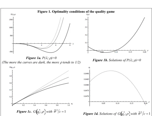
2 (9)— Please insert figure 1 —
For each value of r,
; !
P
( )
l;r has only one real root; !
l r
( )
greater than unity (cf. figure 1a).; !
l r
( )
is a convex function which reaches a minimum at; !
l
(
0.06)
= 5.1731 and exceeds its initial value at; !
r= 0.13!(cf. figure 1b).6 For each value of r, we thus compute the unique associated value
; !
l r
( )
and then substitute; ! l r
( )
ql* for ; ! qh* and ; ! rql* for ; !ge in the second optimality condition (7). We therefore deduce the proposition 2 below.
4
Motta (1993) proves that these qualities are indeed Nash equilibrium.
5
The market is indeed partly covered if
; ! q £ ˜ q!, so that ; ! q! q > 4.706. Moreover, ; ! ql*£ qh* £ 1 if ; ! q!2 c£ 1 0.2533» 3.95. 6
Calculations and simulations were made with the software Mathematica. It is impossible to express the form of this root simply.
Proposition 2. When the emission tax parameter
; !
g
e ºt
e(
q!
+t
e)
is expressed in terms of a percentage r!of the ex post brown quality; !
ql* and
; !
r
Î 0,1 2[ ]
, the equilibrium brown quality; !
ql* is implicitly defined by the following equation:
; ! G q
( )
l*;r º 1-(
rq*l)
2ql*-f r( )
q! 2 c = 0 (10) with ; ! f r( )
=(
1- 2r)
l r( )
(
4.l r( )
- 7)
l r( )
+ 2 4l r( )
2 - 3l r( )
+ 1(
)
r(
)
4.l r( )
-1(
)
3 (11)and the equilibrium green quality is defined as
; !
qh*=l r
( )
ql*.The polynomial function
; !
G q
( )
l*;r
increases in; !
q
l* and has only one real root; !
ql*
( )
rlower than unity, the expression of which is given in appendix A1 (cf. figure 1c).7 The brown quality
; !
ql*
( )
r increases with the tax parameter r and reaches its maximum at; !
ˆ
r!
= 0.07 (cf. figure 1d). Consequently, the green quality, defined by; !
qh*=l r
( )
ql*, may increase or decrease with r!according to the relative importance of the contradictory effects of the differentiation index; !
l r
( )
and the brown quality; !
ql*
( )
r . We show in appendix A1 that these qualities are the only stable solution of the quality game. Moreover, a simulation of both first order conditions, presented in appendix A2, shows that our methodology allows us to select the one stable equilibrium. Although the formulation of the game equilibrium set out in proposition 2 allows us to outline the effects of key parameters of the game on firms’ choices, only simulations enable us to study more thoroughly the implications of the emission tax on the game equilibrium.3.3 The consequences of an emission tax
An analysis of the qualities at the game equilibrium is carried out by restricting the study to the duopoly case, in such a way that definition space of
; !
te becomes
; !
0,t!e
[
]
.8— Please insert figure 2 —
A tighter emission tax leads to an improvement in the brown quality
; !
ql* when
; !
te
remains lower than a given threshold
; !
ˆ
t!e, and to a deterioration beyond this threshold (figure 2a). This result is in line with the proposition 2: the maximal brown quality is obtained with a tax parameter
; !
ˆ
r!
= 0.07, which corresponds to an emission tax; !
ˆ
t!e= 0.004 in our baseline scenario where
; !
q! and c are equal to 1. Furthermore, a more stringent tax tends to enhance the high quality
; !
qh* (figure 2b). As a consequence, differentiation slightly decreases when
; !
te is low but noticeably increases with
; ! te for 7 ; ! G 0;
( )
r = -f r( )
q!2 c < 0 while ; ! f( )
0 > 0, ; ! f r( )
is slightly increasing up to ; ! f(
0.06)
= 0.049, and then decreasing to zero for; ! r= 1 2. 8 For ; ! q! and c equal to 1, ; !
t!e= 0.0085 . Obviously, this threshold rises with
; ! q! ( ; ! t!e= 0.0148 for ; ! q!=1.2, ; ! t!e= 0.0238 for ; ! q!=1.4, ; ! t!e= 0.0362 for ; ! q!=1.6, ; ! t!e= 0.0525 for ; !
q!=1.8) and decreases with
c. It corresponds to a tax parameter
; !
higher values. The differentiation index shape highlighted in the figure 1b corroborates this result: ; ! l r
( )
is minimum at ; ! r= 0.06 such as ; !t
e = 0.003 in our baseline scenario. A higher emission tax increases prices through its direct effect on production cost and its indirect impact on product differentiation. The deterioration of the quality; !
ql*, beyond
; !
ˆ
t!e, however, acts in the opposite direction. For both products, the former effect is stronger than the latter, in such a way that the higher
; !
te is, the higher prices will be (figure 2c and 2d).
Higher emission taxation also tends to reduce demand for brown (figure 2e) and for green quality when
; !
q! remains relatively low (figure 2f). Several variants on this parameter show that when
; !
q! is sufficiently high, the demand for the green variant can grow with the tax (see appendix A4). In this case, the improvement of the green quality is due to a more stringent tax offsetting the price effect. Therefore, green demand follows a bell-shaped curve for medium
; !
q! and a rising curve for higher
; !
q!.
As a consequence, the profit of the brown firm decreases with the emission tax, becoming equal to zero for the tax
; !
t!e (figure 2g). By contrast, the profit of the green firm follows a U-shaped curve thanks to the higher quality of its product (figure 2h). As a result, a high pollution tax leads to a green product monopoly, for which the analysis is given in appendix A3.
We have shown that a low emission tax enhances the quality of both products, and hence the quality of the environment, but increases product differentiation. The contradictory impacts of the tax on both market failures raise the question of its effects on social welfare.
4. The second best optimum
In accordance with the literature on environmental economics, we assume that global pollution generates environmental damage and this corresponds to a monetary valuation of the impact of pollution on society as a whole (Baumol and Oates, 1988). The welfare function is defined in the following way:
;
W = CSh + CSl + ph + pl+ GR - D (12)
with CSi the surplus of consumers purchasing the quality qi, pi the firm i’s profit (i=h,l),
GR the tax revenue and D the environmental damage function. The damage is assumed
to be linear with respect to total emissions E. Let d be the marginal environmental damage, the total damage is then defined by
;
D=
d
E, with;
d
³ 0. We analyze the effects of the emission tax on each component of welfare before inferring its global impact.— Please insert figure 3 —
The net surpluses of consumers of green and brown products are defined by:
; CSi= q
(
q
qi- pi)
dq
i q iò
=1 2qidi(
q
i+q
i)
- pidi i= h,l (13) with ; ql= ˜ q , ; q l =qh= ˆ q and ;q h =q . An increase in the emission tax raises the brown quality (below
;
ˆ
t e) and the green quality but it induces higher prices. Surplus of both types of consumers is reduced because the price effect outweighs the quality effect (figures 3a and 3b).
As shown previously, a brown firm’s profit decreases with the emission tax whereas a green firm’s profit follows a U-shaped curve.
Pollution is defined by:
; E= 1- q
(
h*)
dh*+ 1- q(
l*)
dl* =q
1-r
ql* 3l
-r
(
1+ 2l
)
-l
(
2l
+1- 3r
)
ql* 4l
-1(
)
(14)A rise in the emission tax tends to reduce pollution thanks to an improvement in the ecological quality of products and a drop in the total demand (figure 3c). Nevertheless, the tax revenue, defined by
;
GR=
t
eE, grows with the tax (figure 3d).— Please insert figure 4 —
The effects of the emission tax on global welfare are not a priori obvious. Welfare tends to grow with
;
te thanks to fiscal revenue supplement and pollution reduction, but the loss in consumers’ surpluses and firms’ profit act in the an opposite direction. For a very low marginal damage, welfare follows a concave curve where the maximum is reached for a tax
;
te*
lower than its maximal value
;
t e (figure 4).9 If the marginal environmental damage is higher, welfare is a growing function of
;
te. The welfare is then maximal for the value
;
t e. We indeed show in appendix A3 that green monopoly taxation is always welfare depressing.
Studies of environmental tax in non-competitive markets underline that the second-best optimum is reached with an emission tax lower than the marginal environmental damage. This result is generally verified in our framework. Obviously, when d is higher than the maximal tax
;
t e, the optimal tax is always lower than marginal damage. When
d is lower than the maximal tax
;
t e, simulations with a range of values for
;
q show that the optimal tax remains lower than marginal damage when
;
q is not too high. For instance, when
;
q is normalized to 1, the optimal environmental tax is always lower than the marginal damage, whatever d may be (see footnote 9). However, a special case emerges when
;
q is higher than a threshold, denoted
;
q :10 the fiscal revenue effect is then so great that the optimal environmental tax is positive even with a marginal damage equal to zero. As a consequence, an optimal tax higher than the small marginal damage may arise (cf. appendix A4).
Proposition 3. The higher the marginal damage d is, the higher the second-best optimal emission tax
;
te* will need to be. A marginal damage threshold
;
d and a
ecological awareness threshold
;
q exist such that the optimal tax is lower than marginal damage if:
(a) ;
d
>t
e, then ; te*£t e <d (b) ;d
£t
e and ;q
£q
, then ; te* <d£t e 9In the baseline scenario, the welfare follows a concave curve if d ≤ 0.025 and the maximum is reached for te=0.002 (r = 0.04) if d = 0.01, te=0.007 (r = 0.14) if d = 0.02 and te=0.008 (r = 0.18) if d = 0.025.
10
Our simulations show that
;
(c) ;
d
£t
e, ;q
>q
and ; d³d , then ; te*<d£t eand the optimal tax is higher than the marginal damage if: (d) ;
d
£t
e, ;q
>q
and ; d<d , then ; d£te * £t eBeyond a certain marginal damage, the optimal tax reaches its maximal value
;
t e.
The most polluting firm is also ejected from the market and the less polluting firm becomes a green product monopolist.
Thus an emission tax seems an efficient means to move the game equilibrium closer to the Pareto’s optimum. In most cases, the optimal tax is lower than marginal damage. This environmental policy can lead to a green monopoly. The optimal tax is then the one that induces a kind of limit price strategy for the green monopoly.
5. Conclusion
Since Pigou’s work, environmental tax has been considered as one of the most efficient environmental policies. In a competitive market, the optimal tax is equivalent to the marginal environmental damage and leads to a first best optimum. When polluters compete in a non-competitive market, the environmental tax generally remains an efficient instrument but the coexistence of two market failures for only one policy leads economists to advocate a tax that is less than the marginal damage. This tax allows the attainment of a second-best optimum.
In our paper, we have examined a new non-competitive case:
- environmental quality competition in green markets where consumers differ in their ecological consciousness, and thus in their willingness-to-pay for environmental quality;
- and, polluting duopoly that compete both in price and the environmental quality of their products in a vertically differentiated market.
Furthermore, we have focused on situations where the improvement of environmental quality requires R&D expenditure, and thus involves fixed costs. We have shown that an emission tax leads to a decrease in pollution, through an improvement in green, and, in some cases, brown quality. The tax is therefore successful at increasing overall welfare.
The higher the marginal damage is, the higher the optimal tax will need to be. But the optimal tax is also less than the marginal damage when the market is not too large. In the case of relatively high marginal environmental damage, the optimal emission tax leads to the eviction of the brown product firm by giving an advantage to the green product firm. This is counter to a policy of higher competition between firms. In consequence, it may be advisable to introduce an economical policy to reduce the inefficiency caused by the monopoly power of the green firm.
This paper completes the results from Lombardini-Riipinen (2005), who studies emission tax in the case of variable costs for quality improvement, and Moraga-González and Padrón-Fumero (2002), who consider the effects of unit emission standards, technology subsidies and product tax in the case of fixed costs for quality improvement. In order to extend our analysis, it may be useful to provide some comparative statics of environmental quality, prices and welfare. This requires resolving
difficulties arising from the introduction of a variable cost in a product-differentiation model with fixed cost for quality. This will soon be subject to further research.
6. References
Arora S., Gangopadhyay S. (1995), “Towards a Theoretical Model of Voluntary Overcompliance”, Journal of Economic Behavior and Organization, 28, 289-309. Bansal S., Gangopadhyay (2003), “Tax/subsidy Policies in the Presence of
Environmentally Aware Consumers”, Journal of Environmental Economics and
Management 45, 333-355.
Barnett A. (1980), “The Pigouvian Tax Rule under Monopoly”, American Economic
Review 70, 1037-1041.
Baumol W., Oates W. (1988), The Theory of Environmental Policy, Cambridge University Press.
Brécard D. (2008a), “Une note sur la taxation ad valorem des produits polluants sur un marché vert”, Revue Économique, 59(3).
Cremer H., Thisse J.-F. (1994), “Commodity Taxation in a Differentiated Oligopoly”,
International Economic Review 35(3), 613-633.
Cremer H., Thisse J.-F. (1999), “On the Taxation of Polluting Products in a Differentiated Industry”, European Economic Review 43, 575-594.
Delipalla S., Keen M. J. (1992), “The comparison between ad valorem and specific taxation under imperfect competition”, Journal of Public Economics 49, 351-367. Ebert U. (1992), “Pigouvian Taxes and Market Structure: The Case of Oligopoly and
Different Abatement Technologies”, Finanzarchiv 49, 154-166.
European Commission, 2008. Attitudes of Europeans citizens towards the environment. Eurobarometer 295.
Katsoulacos Y., Xepapadeas A. (1995), “Environmental Policy under Oligopoly with Endogenous Market Structure”, The Scandinavian Journal of Economics 97(3), 411-420
Levin D. (1985), “Taxation within Cournot Duopoly”, Journal of Public Economics 27, 281-290.
Lombardini-Riipinen C. (2005), “Optimal Tax Policy under Environmental Quality Competition”, Environmental and Resource Economics 32, 317-336.
Moraga-González J. L., Padrón-Fumero N. (2002), “Environmental Policy in a Green Market”, Environmental and Resource Economics 22, 419-447
Motta M. (1993), “Endogenous Quality Choice: Price vs. Quantity Competition”, The
Journal of Industrial Economics 41(2), 113-131.
Motta, M., Thisse, J.-F. (1999), “Minimum Quality Standard as an Environmental Policy: Domestic and International Effects”, in Environmental Regulation and
Market Power, E. Petrakis, S. Sartzetakis, and A. Xepapadeas (eds), Edward Elgar,
27-46
Mussa, M. et Rosen, S. (1978), “Monopoly and Product Quality”, Journal of Economic
Theory 18, 301-317.
OCDE (2007), The Political Economy of Environmentally Related Taxes, OCDE, Paris. Pigou A. C. (1920), The Economic of Welfare, MacMillan, London.
Pirtillä J. (2002), “Specific versus ad valorem Taxation and Externalities”, Journal of
Poyago-Theotoky J. A., Teerasuwannajac K. (2002), “The Timing of Environmental Policy : A Note on the Role of Product Differentiation», Journal of Regulatory
Economics, 21(3), 305-316..
Requate T. (1993a), “Pollution Control in a Cournot Duopoly via Taxes or Permits”,
Journal of Economics 58, 255-291.
Requate T. (1993b), “Pollution Control under imperfect Competition: Asymetric Bertrand Dopoly with Linear Technologies”, Journal of Institutional and Theoretical
Economics 149, 415-442.
Requate (1997), “Green Taxes in Oligopoly if the Number of Firms is Endogenous”,
Finanzarchiv 54(2), 261-280.
Requate T. (2007), “Environmental Policy under Imperfect Competition”, in The
International Yearbook Of Environmental And Resource Economics 2006/2007. A Survey of Current Issues, Tietenberg T. and Folmer H. eds, Edgar Elgar, 120-207.
Shaked A., Sutton J. (1982), “Relaxing Price Competition Through Product Differentiation”, Review of Economic Studies 49, 3-14.
Simpson R. D. (1995), Optimal pollution taxes in Cournot duopoly. Environmental and
Resource Economics 9, 359–396.
7. Appendix
A1. Conditions for existence of an equilibrium
We study here the first order conditions (7) of the quality subgame. The first equation of conditions (7) decreases with qh: ; ¶2p h ¶qh2 = -8 q
(
l- 2ge)
[
2ge(
qh- ql)
+ q(
l- 2ge)
ql+ 5q(
h-ge)
ql]
q 2 1-ge(
)
(
4qh- ql)
2 - c < 0 as the first term in the numerator is positive and the term in brackets is positive. Moreover,;
¶ph ¶qh q
h= 0
=ge
(
4q ql - 7ge)
ql2> 0when condition (5) is met. There is thus a solution
;
qh*
( )
ql for the first equation (7)The second equation of conditions (7) increases for low values of ql and then decreases for large values of ql. (figure A1) The second derivative of firm l’s profit is:
; ¶2p l ¶ql2 = -2qh
[
4 16q(
h3-16qh2ql+ 6qhql2- 3ql3)
ge2- 4 5q(
h+ ql)
ql3ge- 8q(
h+ 7ql)
qhql3]
q 2 1-ge(
)
(
4qh- ql)
2ql3 - c A solution exists if there is; v> 0 such that ; ¶2p l
( )
v ¶ql 2= 0and ; ¶pl( )
v ¶ql > 0. Some numericalsimulations allow us to show that two equilibria are possible. However, the first one, with the lowest quality, is not stable because firm l’s profit increases for a quality slightly higher than this point. Only the second one is then a stable solution of the second condition (7). Nevertheless, the existence of an equilibrium requires a tax parameter lower than a threshold
;
g e. This threshold is all the more high as the
maximal marginal willingness to pay is high. For
;
q =1 and c=1, the threshold
;
g e is equal 0.011.
Simulations in subsection A2 show that our methodology for game resolution enables us to select the stable equilibrium. The expression of the low quality at equilibrium is given by:
; ql*= 2 3r+ 213 3r -2 + 27b+ 312b 1 2
(
-4 + 27b)
1 2 é ë ê ù û ú 1 3 + -2 + 27b+ 312b 1 2(
-4 + 27b)
1 2 é ë ê ù û ú 1 3 3.213.r with ; b = rf r( )
q 2 c(a)
;
q =1 (b)
;
q =2 Figure A1. Simulation of
;
¶pl ¶ql for qh=0.25
;
ge=0 (clear grey curve), 0.005 (dark grey curve) and 0.01 (black curve)
A2. Simulations of the game equilibrium
The assumption on the value of
;
q affects the scale of the equilibrium qualities, prices and profits: the higher
;
q is, the higher the qualities, the prices and the profits are. The assumptions on the values of c act in the opposite direction: the higher c is, the lower the qualities, the prices and the profits are. Without loss of generality in the analysis of the effects of the emission tax, all the model simulations are then made with the value 1 for
;
q and c.
Tab. A1 Direct simulations of first order conditions
te 0 0.002 0.004 0.006 0.008 ge 0 0.002 0.004 0.006 0.008 ; ql* 0.0482 0.0492 0.0492 0.0487 0.0472 ; qh* 0.2533 0.2542 0.2549 0.2556 0.2562 ; pl* 0.0102 0.0115 0.0126 0.0136 0.0144 ; ph* 0.1077 0.1090 0.1106 0.1125 0.1146 ; dl* 0.2625 0.2418 0.2210 0.1994 0.1754 ; dh* 0.5250 0.5243 0.5233 0.5220 0.5202 ; pl * 0.0015 0.0011 0.0007 0.0004 0.0001 ; p*h 0.0244 0.0241 0.0238 0.0237 0.0237
Tab. A2 Simulations of first order conditions with
; rºge ql * r 0 0.04 0.08 0.12 0.18 f(r) 0.0482 0.0488 0.0488 0.0482 0.0459 l0 5.2512 5.1837 5.1790 5.2419 5.4893 ge 0 0.0020 0.0039 0.0059 0.0084 ; ql * 0.0482 0.0490 0.0492 0.0487 0.0467 ; qh* 0.2533 0.2542 0.2549 0.2556 0.2563 ; pl * 0.0102 0.0114 0.0125 0.0135 0.0145 ; ph* 0.1077 0.1090 0.1106 0.1124 0.1152 ; dl * 0.2625 0.2421 0.2115 0.2007 0.1690 ; dh* 0.5250 0.5243 0.5234 0.5221 0.5196 ; pl * 0.0015 0.0011 0.0007 0.0004 0 ; p*h 0.0244 0.0241 0.0238 0.0237 0.0237
A3. The monopoly case
The emission tax can exclude the standard product firm from a green market. In that case, the green product monopoly faces demand
;
dm=q - pm qm and determines price and quality that maximize its profit: ; pm= 1 tv pm-te
(
1 - qm)
(
)
q - pm qm æ è ç ö ø ÷ -1 2cqm 2The optimal price is
;
pm=1
2
[
te+(
q -te)
qm]
. It’s an increasing function of quality if ;te<q .
Substituting the optimal price into the profit expression leads to the following profit equation:
; pm=te2
(
1 - qm)
2- 2q t e(
1 - qm)
+q 2qm2 4qm -1 2cqm 2The optimal quality is then solution of the first order condition of profit maximization:
;
4cqm3 -
(
q +te)
2qm2 +te2= 0 or ;4cqm3
(
1-ge)
2-q 2qm2+q 2ge= 0. Without emission tax, the monopoly produces the quality;
qm0 =q 2 4c . With a positive emission tax, the optimal green quality of the monopoly is then defined by:
; qm* = bm 3 + 213b m 2 3 -2bm2 + 27b mge+ 3 3 2b mge 1 2 -4b m 2 + 27g e
(
)
1 2 é ë ê ù û ú 1 3 + -2bm2 + 27b mge+ 3 3 2b mge 1 2 -4b m2 + 27ge(
)
1 2 é ë ê ù û ú 1 3 3.213 with ; bm= q 2 4c 1 -(
ge)
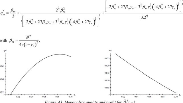
2.Figure A3. Monopoly’s quality and profit for
;
q c= 1
Some numerical simulations allow us to show that
;
qm* increases with ge until a given threshold and then decreases, the demand for green product and the monopoly’s profit decrease with ge. As a consequence, all components of welfare except government revenue tend to decrease with ge in such a way that the emission tax is welfare decreasing.
A comparison between welfare levels in the duopoly case and in the monopoly case highlights that the optimal emission is the one that ousts the brown firm when marginal damage is sufficiently high.
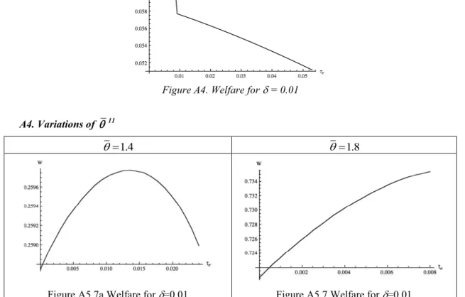
Figure A4. Welfare for d = 0.01 A4. Variations of ; q 11 ; q =1.4 ; q =1.8
Figure A5.7a Welfare for d=0.01 Figure A5.7 Welfare for d=0.01
11
Given the size of image files, only welfare results are reproduced here, but more results are available on request from the authors.
FIGURES
Figure 1. Optimality conditions of the quality game
Figure 1a. P(l; r)=0
(The more the curves are dark, the more r tends to 1/2) Figure 1b. Solutions of P(l; r)=0
Figure 1c.
;
G q
( )
l*;r with ;q 2 c= 1
(The more the curves are dark, the more r tends to 1/2) Figure 1d. Solutions of
;
G q
( )
l*;r with ;Figure 2. The effects of an emission tax te (for ; q 2 c= 1) Figure 2a Figure 2b Figure 2c Figure 2d Figure 2e Figure 2f Figure 2g Figure 2h
Figure 3. The effects of an emission tax on welfare components (for
;
q 2 c= 1)
Figure 3a. Brown consumers’ surplus Figure 3b. Green consumers’ surplus
Figure 3c. Pollution Figure 3d. Tax Revenue
Figures 4. The global effect of an emission tax te on welfare (for
;
q 2 c= 1)