HAL Id: hal-00927400
https://hal.inria.fr/hal-00927400
Submitted on 13 Jan 2014
HAL is a multi-disciplinary open access
archive for the deposit and dissemination of
sci-entific research documents, whether they are
pub-lished or not. The documents may come from
teaching and research institutions in France or
abroad, or from public or private research centers.
L’archive ouverte pluridisciplinaire HAL, est
destinée au dépôt et à la diffusion de documents
scientifiques de niveau recherche, publiés ou non,
émanant des établissements d’enseignement et de
recherche français ou étrangers, des laboratoires
publics ou privés.
Interpretation
Martin Bodin, Thomas Jensen, Alan Schmitt
To cite this version:
Martin Bodin, Thomas Jensen, Alan Schmitt. Pretty-big-step-semantics-based Certified Abstract
Interpretation. JFLA - 25ème Journées Francophones des Langages Applicatifs - 2014, Jan 2014,
Fréjus, France. �hal-00927400�
Certified Abstract Interpretation
Martin Bodin
1,2, Thomas Jensen
2, & Alan Schmitt
21: ENS Lyon; 2: Inria; [email protected]
Résumé
We present a technique for deriving semantic program analyses from a natural semantics specification of the programming language. The technique is based on the pretty-big-step semantics approach applied to a language with simple objects called O’While. We specify a series of instrumentations of the semantics that makes explicit the flows of values in a program. This leads to a semantics-based dependency analysis, at the core, e.g., of tainting analysis in software security. The formalization is currently being done with the Coq proof assistant.1
1.
Introduction
David Schmidt gave an invited talk at the 1995 Static Analysis Symposium [11] in which he argued for using natural semantics as a foundation for designing semantic program analyses within the abstract interpretation framework. With natural (or “big-step” or “evaluation”) semantics, we can indeed hope to benefit from the compositional nature of a denotational-style semantics while at the same time being able to capture intentional properties that are best expressed using an operational semantics. Schmidt showed how a control flow analysis of a core higher-order functional language can be expressed elegantly in his framework. Subsequent work by Gouranton and Le Métayer showed how this approach could be used to provide a natural semantics-based foundation for program slicing [13].
In this paper, we will pursue the research agenda set out by Schmidt and investigate further the systematic design of semantics-based program analyses based on big-step semantics. Two important issues here will be those of scalability and mechanization. The approach worked nicely for a language whose semantics could be defined in 8 inference rules. How will it react when applied to full-blown languages where the semantic definition comprises hundreds of rules? Strongly linked to this question is that of how the framework can be mechanized and put to work on larger languages using automated tool support. In the present work, we investigate how the Coq proof assistant can serve as a tool for manipulating the semantic definitions and certifying the correctness of the derived static analyses.
Certified static analysis is concerned with developing static analyzers inside proof assistants with the aim of producing a static analyzer and a machine-verifiable proof of its semantic correctness. One long-term goal of the work reported here is to be able to provide a mechanically verified static analysis for the full JavaScript language based on the Coq formalization developed in the JSCert project [1]. JavaScript, with its rich but sometimes quirky semantics, is indeed a good raison d’être for studying certified static analysis, in order to ensure that all of the cases in the semantics are catered for.
In our development, we shall take advantage of some recent developments in the theory of operational semantics. In particular, we will be using a particular format of natural semantics call
1This work has been presented at the Festschrift for David Schmidt in September 2013. This work has been partially
supported by the French National Research Agency (ANR), project Typex ANR-11-BS02-007, and by the Laboratoire d’excellence CominLabs ANR-10-LABX-07-01.
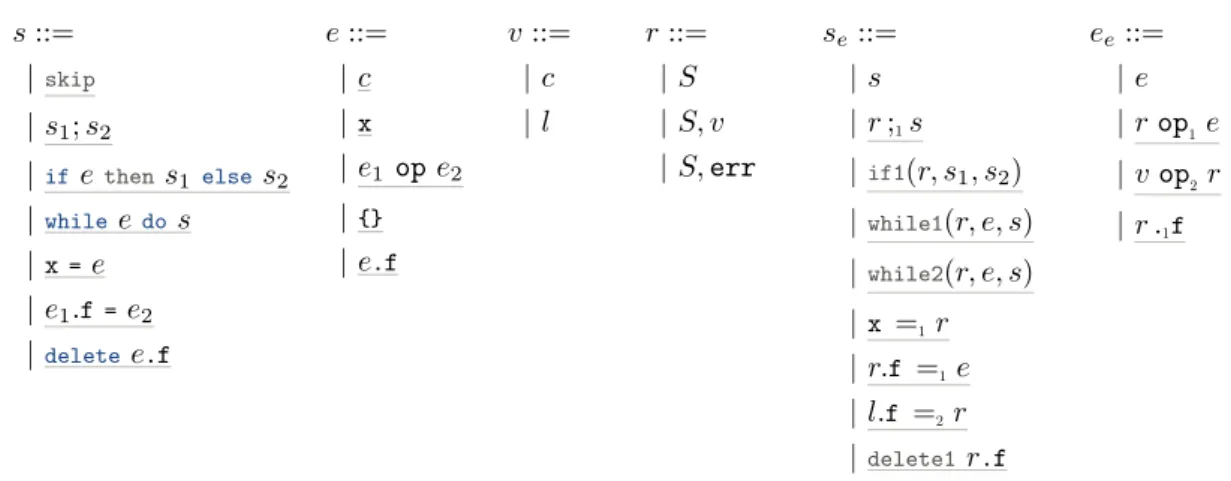
s ::= |skip | s1; s2 |ifethens1 else s2 |whileedos |x= e | e1.f= e2 |delete e.f e ::= | c |x | e1 ope2 |{} | e.f v ::= | c | l r ::= | S | S, v | S, err se::= | s | r ;1s |if1(r, s1, s2) |while1(r, e, s) |while2(r, e, s) |x =1r | r.f =1e | l.f =2r |delete1 r.f ee::= | e | r op1e | v op2r | r .1f
Figure 1: O’While Syntax, Values, Results, and Extended Syntax
“pretty-big-step” semantics [3] which is a streamlined form of operational semantics retaining the format of natural semantics while being closer to small-step operational semantics.
Even though it is our ultimate goal, JavaScript is far too big to begin with as a goal for analysis: its pretty-big-step semantics contains more than half a thousand rules! We will thus start by studying a much simpler language, called O’While, which is basically a While language with simple objects in the form of extensible records. This language is quite far from JavaScript, but is big enough to catch some issues of the analyses of JavaScript objects. We present the language and its pretty-big-step semantics in Section 2. To test the applicability of the approach to defining static analyses, we have chosen to formalize a data flow dependency analysis as used, e.g., in tainting [12] or “direct information-flow” analyses of JavaScript [15, 5]. The property we ensure is defined in Section 3 and the analysis itself is defined in Sections 4. As stated above, the scalability of the approach relies on the mechanization that will enable the developer of the analyses to prove the correctness of analyses with respect to the semantics, and to extract an executable analyzer. We show how the Coq proof assistant is currently being used to formally achieve these objectives as we go along.
2.
O’While
and its Pretty Big Step Semantics
As big-step semantics, pretty-big-step semantics directly relates terms to their results. However, pretty-big-step semantics avoids the duplication associated with big-step semantics when features such as exceptions and divergence are added. Since duplication in the definitions often leads to duplication in the formalization and in the proofs, an approach based on a pretty-big-step semantics allows to deal with programming languages with many complex constructs. (We refer the reader to Charguéraud’s work on pretty-big-step semantics [3] for detailed information about this duplication.) Even though the language considered here is not complex, we have been using pretty-big-step semantics exclusively for our JavaScript developments, thus we will pursue this approach in the present study.
The syntax of O’While is presented in Figure 1. Two new constructions have been added to the syntax of expressions for the usual While language: {}creates a new object, and e.faccesses a field of an object. Regarding statements, we allow the addition or the modification of a field to an object using e1.f=e2, and the deletion of the field of an object usingdeletee.f. In the following we write t
for terms, i.e., both expressions and statements.
we only consider boolean primitive values. The state of a program contains both an environment E, which is a mapping from variables to values, and a heap H, which is a mapping from locations to objects, that are themselves mappings from fields to values. In the following, we write S for E, H when there is no need to access the environment nor the heap. Results r are either a state S, a pair of a state and value S, v, or a pair of an error and a state S, err.
Figure 1 also introduces extended statements and extended expressions that are used in O’While’s pretty-big-step semantics, presented in Figure 2. Extended terms te comprise extended statements
and expressions. Reduction rules have the form S, te → r. The result r can be an error S′, err.
Otherwise, if te is an extended statement, then r is a state S′, and if te is an extended expression,
then r is a pair of a state S′ and returned value v. We write st(r) for the state S in a result r.
Most rules are the usual While ones, with the exception that they are given in pretty-big-step style. We now detail the new rules for expressions and statements. Rule Obj associates an empty object to a fresh location in the heap. Rule Fld for the expression e.ffirst evaluates e to some result r, then calls the rule for the extended expression r .1f. The rule for this extended expression is only
defined if r is of the form E′, H′, l where l is a location in H′ that points to an object o containing a
field f. The rules for field assignment and field deletion are similar: we first evaluate the expression
that defines the object to be modified, and in the case it actually is a location, we modify this object using an extended statement.
Finally, our semantics is parameterized by a partial function abort(·) from extended terms to results, that indicates when an error is to be raised or propagated. More precisely, the function abort(te) is defined at least if te is an extended term containing a subterm equal to S, err for some
S. In this case abort(te) = S, err. We can then extend this function to define erroneous cases. For
instance, we could say that abort((E, H, v).f =1e) = E, H, err if v is not a location, or if v = l but l
is not in the domain of H, or iffis not in the domain of H[l]. This function is used in the Abort rule,
that defines when an error is raised or propagated. This illustrates the benefit of a pretty-big-step semantics: a single rule covers every possible error propagation case.
The derivation in Figure 14 in Appendix B is an example of a derivation of the semantics.
3.
Annotated Semantics
3.1.
Execution traces
We want to track how data created at one point flows into locations (variables or object fields) at later points in the execution of the program. To this end, we need a mechanism for talking about “points of time” in a program execution. This information is implicit in the semantic derivation tree corresponding to the execution. To make it explicit, we instrument the semantics to produce a (linear) trace of the inference rules used in the derivation, and use it to refer to particular points in the execution. As every other instrumentation in this paper, it adds no information to the derivation but allows global information to be discussed locally.
More precisely, we add partial traces, τ ∈ Trace, to both sides of the reduction rules. These traces are lists of names used in the derivation. The two crucial properties from traces is that they uniquely identify a point in the derivation (i.e., a rule in the tree and a side of this rule), and that one may derive from the trace the syntactic program point that is being executed at that point.
Since traces uniquely identify places in a derivation, we use them from now on to refer to states or further instrumentation in the derivation. More precisely, if τ is a trace in a given derivation, we write Eτ and Hτ for the environment and heap at that point.
S,skip→ S Skip S, s1→ r S, r ;1s2→ r ′ S, s1; s2→ r′ Seq S ′, s → r S, S′; 1s → r Seq1 S, e→ r S,if1(r, s1, s2) → r′ S,ifethens1 elses2→ r′ If S ′, s 1→ r S,if1((S′,true), s 1, s2) → r IfTrue S′, s 2→ r S,if1((S′,false), s 1, s2) → r IfFalse S, e → r S,while1(r, e, s) → r ′ S,whileedos → r′ While S′, s → r S′,while2(r, e, s) → r′
S,while1((S′,true), e, s) → r′ WhileTrue1
S′,whileedos → r
S,while2(S′, e, s) → r WhileTrue2
S,while1((S′,false), e, s) → S′ WhileFalse
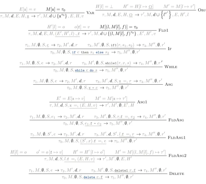
E, H, e → r E, H,x =1r→ r′ E, H,x= e → r′ Asg E′= E[x7→ v] S,x =1(E, H, v) → E′, H Asg1 S, e1→ r S, r.f =1e2→ r ′ S, e1.f=e2→ r′ FldAsg S′, e → r S′, l.f = 2r→ r′ S, (S′, l).f = 1e → r′ FldAsg1 H[l] = o o ′= o [f7→ v] H′= H [l 7→ o′] S, l.f =2(E, H, v) → E, H′ FldAsg2 S, e→ r S,delete1r.f→ r′ S,deletee.f→ r′ Del H[l] = o o[f] ̸= ⊥ o′ = o [f7→ ⊥] H′= H [l 7→ o′] S,delete1(E, H, l).f→ E, H′ Del1 S, c → S, c Cst E[x] = v E, H,x→ E, H, v Var S, e1→ r S, r op1e2→ r′ S, e1ope2→ r′ Bin S ′, e 2→ r S′, v1op2r → r′ S, (S′, v 1) op1e2→ r′ Bin1 v = v1opv2 S, v1op2(S, v2) → S, v Bin2 H[l] = ⊥ H ′= H[l 7→{}] E, H,{}→ E, H′, l Obj S, e→ r S, r .1f→ r ′ S, e.f→ r′ Fld H′[l] = o o[f] = v E, H, (E′, H′, l) . 1f→ E′, H′, v Fld1 abort(te) = r S, te→ r Abort
3.2.
A General Scheme to Define Annotations
In principle, the annotation process takes as argument a full derivation tree and returns an annotated tree. However, every annotation process we define in the following, as well as the one deriving traces, can be described by an iterative process that takes as arguments previous annotations and the parameters of the rule applied, and returns an annotated rule.
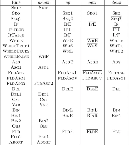
More precisely, our iterative process is based on steps of four kinds: axiom steps (for axioms), that transform the annotations on the left of axiom rules into annotations on the right of the rule, up steps (for rules with inductive premises), that propagate an annotation on the left of a rule to its first premise, down steps (for rules with inductive premises), that propagate an annotation on the right of the last premise to the right of the rule, and next steps (for rules with two inductive premises), that propagate the annotations from the left of the current rule and from the right of the first premise into the left of the second premise. As we are using a pretty-big-step semantics, there are at most two inductive premises above each rule, thus these steps are sufficient.
.. a1 → a..2 .. a4 → a..5 .. a3 → a..6 .. a0 → a..7 .. axiom . axiom . up . up . down . down .. next This generic approach allows to compose complex
annotations, building upon previously defined ones. This general scheme is summed up on the right, where each ai
represents an annotation. The colors show which steps are associated to which rules: a0 is the initial annotation. It is
changed to a1 and control is passed to the left axiom rule
(black up). The blue axiom step creates a2, and control returns to the bottom rule, where the black
next step combines a2 and a0 to pass it to the red rule. Annotations are propagated in the right
premise, and ultimately control comes back to the black rule which pulls the a6 annotation from the
red rule and creates its a7annotation. Note that the types of the annotations on the left and the right
of the rules do not have to be the same, as long as every left-hand side annotation has the same type, and the same for right-hand side annotations.
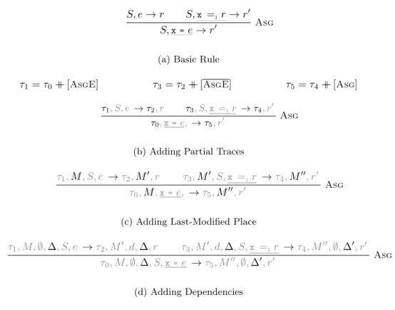
As an example, we define the axiom, up, down, and next steps corresponding to the addition of partial traces for rules Var and Asg (see Figure 3b and 4b). Rule Var illustrates the axiom step, that adds a Var token at the end of the trace. Rule Asg illustrates the other steps: adding a AsgE as up step, adding a AsgE as next step, and adding Asg as down step. We fully describe in Appendix A.2 how the traces are added following this approach.
3.3.
Dependency Relation
We are interested in deriving the dependency analysis underlying tainting analyses for checking that secret values do not flow into other values that are rendered public. To this end, we consider direct flows from sources to stores. We need a mechanism for describing when data was created and when a flow happened, so we annotate locations in the heap with the time when they were allocated. By “time” we here mean the point of time in an execution, represented by a trace τ of the derivation. We write ALoc = Loc × Trace for the set of annotated locations. Similarly, we annotate variables and fields with the point in time that they were last assigned to. When describing a flow, we talk about sources and stores. Sources are of three kinds: an annotated location, a variable annotated with its last modification time, or a pair of annotated location and field further annotated with their last modification time. Stores are either a variable or a pair of an annotated location and a field, further annotated with their last modification time. Formally, we define the following dependency relation
⊂
. ∈ Dep = P (Source × Store)
where Store = (Var × Trace) + (ALoc × Field × Trace) and Source = ALoc + Store. For instance, we write yτ1.⊂
xτ2 to indicate that the content that was put in the variable
y at
Var E[x] = v
E, H,x→ E, H, v (a) Basic Rule
E[x] = v τ′= τ ++ [Var]
E, H,τ,x →E, H,τ′, v
Var
(b) Adding Partial Traces
Var E[x] = v τ
′ = τ ++ [Var]
E, H, τ,M,x →E, H, τ′,M, v
(c) Adding Last-Modified Place
E[x] = v τ′= τ ++ [Var] M [x] = τ
0
E, H, τ, M,x →E, H, τ′, M,{xτ0}
, v Var (d) Adding Dependencies
Figure 3: Instrumentation Steps for Var
lτ2. l⊂ ′τ1
.fτ3 to indicate that the object allocated at location l at time τ
2 flows at time τ3 into fieldf
of location l′ that was allocated at time τ1.
3.4.
Direct Flows
We now detail how to compose additional annotations to define our direct flow property . . As flows⊂ are a global property of the derivation, we use a series of annotations to propagate local information until we can locally define direct flows.
We first collect in the derivation the traces where locations are created and where variables or object fields are assigned. To this end, we define a new annotation M of type (Loc + Var + ALoc × Field ) → Trace. After this instrumentation step, reductions are of the form τ, Mτ, Sτ, t → τ′, Mτ′, r. Note that
the trace in information in ALoc× Field is redundant in our setting, as locations may not be reused. It is however useful when showing the correspondence with the analyses as the trace information lets us derive the program point at which the location was allocated.
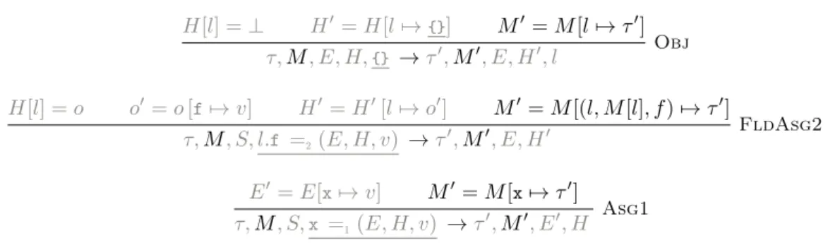
The three rules that modify M are Obj, Asg1, and FldAsg2. We describe them in Figure 5. The other rules simply propagate M . For the purpose of our analysis, we do not consider the deletion of a field as its modification. More precise analyses, in particular ones that also track indirect flows, would need to record such events.
The added instrumentation uses traces to track the moments when locations are created, and when fields and variables are assigned. For field assignment, the rule FldAsg2 relies on the fact that the location of the object assigned has already been created to obtain the annotated location: we have the invariant that if H[l] is defined, then M [l] is defined.
We can now continue our instrumentation by adding dependencies d ∈ P (Var ). The instrumented reduction is now τ, Mτ, dτ, Sτ, t → τ′, Mτ′, dτ′, r. Its rules are described in Figure 6. The rules not
given only propagate the dependencies. The intuition behind these rules is that expressions generate potential dependencies that are thrown away when they don’t result in direct flow (for instance when computing the condition of a If statement). The important rules are Var, where the result depends on the last time the variable was modified, Obj, which records the dependency on the creation of the object, and Fld1, whose result depends on the last time the field was assigned. The Asg and FldAsg1 rules make sure these dependencies are transmitted to the inductive call to the rule that will proceed with the assignment for the next series of annotations.
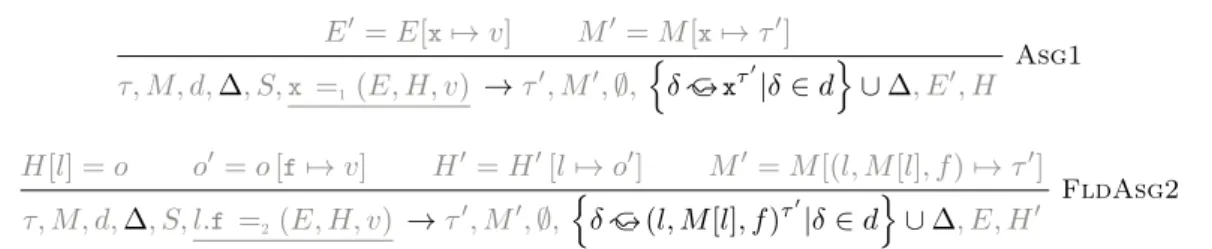
Finally, we build upon this last instrumentation to define flows. The final instrumented derivation is of the form: τ, Mτ, dτ, ∆τ, Sτ, s → τ′, Mτ′, dτ′, ∆τ′, rτ′, where {∆τ, ∆τ′} ⊆ Dep are sets of flows
defining the .⊂ relation (see Section 3.3). The two important rules are Asg1 and FldAsg2, which modify respectively a variable and a field, and for which the flow needs to be added. All the other
S, e → r S,x =1r → r′
S,x=e → r′
Asg
(a) Basic Rule
τ1= τ0++ [AsgE] τ3= τ2++ [AsgE] τ5= τ4++ [Asg]
τ1, S, e →τ2, r τ3, S, x =1r →τ4, r′
τ0, x=e, →τ5, r′
Asg
(b) Adding Partial Traces
τ1,M, S, e →τ2,M′, r τ3,M′, S,x =1r →τ4,M′′, r′
τ0,M,x=e, →τ5,M′′, r′
Asg
(c) Adding Last-Modified Place
τ1, M, ∅,∆, S, e →τ2, M′, d,∆, r τ3, M′, d,∆, S,x =1r →τ4, M′′, ∅,∆′, r′
τ0, M, ∅,∆, S,x=e →τ5, M′′, ∅,∆′, r′
Asg
(d) Adding Dependencies
Figure 4: Instrumentation Steps for Asg
rules just propagate those new constructions. The two modified rules are given in Figure 7.
3.5.
Correctness Properties of the Annotations
The instrumentation of the semantics does not add information to the reduction but only makes existing information explicit. The correctness of the instrumentation can therefore be expressed as a series of consistency properties between the different instrumented semantics.
We first state correctness properties about the instrumentation of the heap. We start by a property concerning the last-modified-place annotations. This property states that the annotation of a location’s creation point never changes, and that the value of a field has not changed since the point of modification indicated by the instrumentation component M .
Property 1 For every instrumented tree, and for every rule in this tree τ, Mτ, Eτ, Hτ, t → τ′, Mτ′, r
where st(r) = Eτ′, Hτ′ and Mτ′[lτ0.f] = τ1; we have Mτ′[l] = τ0 and Hτ′[l][f] = Hτ1[l][f].
The following property links the last-change-place annotation (M ) with the dependencies annotation (∆). Intuitively, it states that if ∆ says that the value assigned to x at time τ1 later
flew into a variable a time τ2 then x has not changed between τ1and τ2.
Property 2 For every instrumented tree, and for every rule in this tree s, τ, Mτ, dτ, ∆τ, Sτ, t →
τ′, M
τ′, dτ′, ∆τ′, r if xτ1.⊂yτ2 ∈ ∆τ′, then at time τ2, the last write to x was at time τ1, i.e.,
Mτ2[x] = τ1.
We now state the most important property: if at some point during the execution of a program the field of an object contains another object, then there is a chain of direct flows attesting it in the
H[l] = ⊥ H′ = H[l 7→{}] M′= M [l 7→ τ′] τ,M, E, H,{} →τ′,M′, E, H′, l Obj H[l] = o o′= o [f7→ v] H′ = H′[l 7→ o′] M′= M [(l, M [l], f ) 7→ τ′] τ,M, S, l.f =2(E, H, v) →τ′,M′, E, H′ FldAsg2 E′ = E[x7→ v] M′ = M [x7→ τ′] τ,M, S,x =1(E, H, v) →τ′,M′, E′, H Asg1
Figure 5: Adding Modified and Created Information
annotation. More precisely, we write l0.⊂∗∆ln.f if there are stores s0 . . . sn such that: s0 = lτ00 for
some τ0, sn= lτnn.fτ
′
nfor some τ
nand τn′, and for every i in [1..n] we have either si= lτii.fiτ
′
i for some
li,fi, τi, and τi′ or si=xiτ
′
i for some x
i and τi′; and for every i, si. s⊂ i+1 ∈ ∆.
Property 3 For every instrumented tree, and for every rule in this tree τ, Mτ, dτ, ∆τ, Eτ, Hτ, t →
τ′, M
τ′, dτ′, ∆τ′, r where st(r) = Eτ′, Hτ′, we have: for every locations l, l′ and field f such that
Hτ[l′][f] = l, then l ⊂. ∗∆τl
′.f; for every locations l, l′ and fieldfsuch that H
τ′[l′][f] = l, then l ⊂. ∗∆ τ′l
′.f.
3.6.
Annotated Semantics in Coq
In the Coq development, we distinguish expressions from statements, and we define the reduction→ as two Coq predicates: red_expr and red_stat. The first predicate has type environment→heap→
ext_expr→out_expr→Type (and similarly for the statement reduction). The construction ext_expr refers to the extended syntax for expressions ee. The inductive typeout_expris defined as being either
the result of a terminating evaluation, containing a new environment, heap, and returned value, or an aborted evaluation, containing a new environment and heap.
1 Inductiveout_expr:=
2 | out_expr_ter:environment→heap_o→value→out_expr
3 | out_expr_error:environment →heap_o→out_expr.
To ease the instrumentation, we directly add the annotations in the semantics: each rule of the semantics takes two additional arguments: the left-hand side annotation and the right-hand side annotation. However, there is no restriction on these annotations, we rely on the correctness properties of Section 3.5 to ensure they define the property of interest.
The semantics is thus parameterized by four types, corresponding to the left and right annotations for expressions and statements. These types are wrapped in a Coq record and used through projections such asannot_e_l(for left-hand-side annotations in expressions).
Figure 8 shows the rule for variables from this annotated semantics, where ext_expr_expr corresponds to the injection of expressions into extended expressions. The additional annotation arguments of type annot_e_l and annot_e_rare carried by every rule. As every rule contains such annotations, it is easy to write a function extract_anottaking such a derivation tree and returning the corresponding annotations. Every part of the Coq development that uses the reduction → but not the annotations (such as the interpreter) uses trivial annotations of unit type.
The annotations are then incrementally computed using Coq functions. Each of the new annotating passes takes the result of the previous pass as an argument to add its new annotations. The initial annotation is the trivial one, where every annotating types are unit. The definition of
E[x] = v M [x] = τ0 τ, M,d, E, H,x →τ′, M,d ∪ {xτ0}, E, H, v Var H[l] = ⊥ H′ = H[l 7→{}] M′= M [l 7→ τ′] τ, M,d, E, H,{} →τ′, M,d ∪ { lτ′} , E, H′, l Obj H′[l] = o o[f] = v M [(l, M [l], f )] = τ 0 τ, M,d, E, H, (E′, H′, l) .1f →τ′, M,d ∪ {(l, M [l], f )τ0}, E′, H′, v Fld1 τ1, M,∅, S, e →τ2, M′,d, r τ3, M′,∅, S,if1(r, s1, s2) →τ4, M′′,∅, r′ τ0, M,∅, S,ifethens1 else s2 →τ5, M′′,∅, r′ If τ1, M,∅, S, e →τ2, M′,d, r τ3, M′,∅, S,while1(r, x, s) →τ4, M′′,∅, r′ τ0, M,∅, S,whileedos →τ5, M′′,∅, r′ While τ1, M,∅, S, e →τ2, M′,d, r τ3, M′,d, S,x =1r →τ4, M′′,∅, r′ τ0, M,∅, S,x= e →τ5, M′′,∅, r′ Asg E′= E[x7→ v] M′= M [x7→ τ′] τ, M,d, S,x =1(E, H, v) →τ′, M′,∅, E′, H Asg1 τ1, M,∅, S, e1 →τ2, M′,d, r τ3, M′,∅, S, r.f =1e2 →τ4, M′′,∅, r′ τ0, M,∅, S, e1.f=e2 →τ5, M′′,∅, r′ FldAsg τ1, M,∅, S′, e →τ2, M′,d, r τ3, M′,d, S′, l.f =2r →τ4, M′′,∅, r′ τ0, M,∅, S, (S′, x).f =1e →τ5, M′′,∅, r′ FldAsg1 H[l] = o o′= o [f7→ v] H′= H′[l 7→ o′] M′= M [(l, M [l], f ) 7→ τ′] τ, M,d, S, l.f =2(E, H, v) →τ′, M′,∅, E, H′ FldAsg2 τ1, M,∅, S, e →τ2, M′,d, r τ3, M′,∅, S,delete1 r.f →τ4, M′′,∅, r′ τ0, M,∅, S,deletee.f →τ5, M′′,∅, r′ Delete
Figure 6: Rules for Dependencies Annotations
annotations in our Coq development exactly follows the scheme presented in Section 3.2. This allows to only specify the parts of the analysis that effectively change their annotations, using a pattern matching construction ending with a Coq’s wild card_to deal with all the cases that just propagate the annotations. It has been written in a modular way, which is robust to changes. For example, a previous version of the annotations only modified partial traces on one side of the rules. As all the following annotating passes treat the traces as an abstract object whose type is parameterized, it was straightforward to update the Coq development to change traces on both sides of each rule.
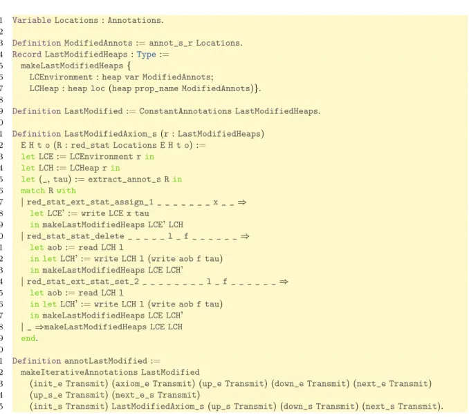
Figure 9 shows the introduction of the last-modified annotation (see Figure 3c and 4c). This annotation is parameterized by another (traces for instance) here calledLocations. In Coq, the heap M of Section 3.4 is represented by the recordLastChangeHeapsdefined on Line 4. Line 9 then states it is the left and right annotation types of this annotation. Next is the pattern matching defining the axiom rule for statement, and in particular the case of the assignment Line 17 which, as in Figure 4c, stores the current location τ in the annotation. Line 31 sums up the rules, stating that every rule
E′= E[x7→ v] M′= M [x7→ τ′] τ, M, d,∆, S,x =1(E, H, v) →τ′, M′, ∅, { δ ⊂. xτ′|δ ∈ d } ∪ ∆, E′, H Asg1 H[l] = o o′= o [f7→ v] H′= H′[l 7→ o′] M′= M [(l, M [l], f ) 7→ τ′] τ, M, d,∆, S, l.f =2(E, H, v) →τ′, M′, ∅, { δ ⊂. (l, M [l], f )τ′|δ ∈ d}∪ ∆, E, H′ FldAsg2
Figure 7: Rules for Annotating Dependencies of Statements 1 Inductivered_expr:environment →heap_o→ext_expr→out_expr→Type:=
2 (* ... *)
3 | red_expr_expr_var:annot_e_l Annots→annot_e_r Annots→
4 ∀E H x v, getvalue E x v→red_expr E H (ext_expr_expr(expr_var x)) (out_expr E H v)
Figure 8: A Semantic Rule as Written in Coq
of this annotation just propagates their arguments, except the axiom rule for statements. As can be seen, the corresponding code is fairly short.
We have also defined an interpreter run_expr:nat→environment→heap_o→expr→option out taking as arguments an integer, an environment, a heap, and an expression and returning an output. The presence of awhilein O’While allows the existence of non-terminating executions, whereas every Coqfunction must be terminating. To bypass this mismatch, the interpretersrun_exprandrun_stat (respectively running over expressions and statements) take an integer (the first argument of type natabove), called fuel. At each recursive call, this fuel is decremented, the interpreter giving up and returningNoneonce it reaches 0. We have proven the interpreter is correct related to the semantics, and we have extracted it as an OCaml program using the Coq extraction mechanism.
4.
Dependency Analysis
The annotating process makes the property we want to track appear explicitly in derivation trees. Our next step is to define an abstraction of the semantics for computing safe approximations of these properties, and to prove its correctness with respect to the instrumented semantics.
4.1.
Abstract Domains
The analysis is expressed as a reduction relation operating over abstractions of the concrete semantic domains. The notion of program point will play a central role, as program points are used both in the abstraction of points of allocation and points of modification. This analysis thus uses the set PP of program points, so we assume that the input program is a result of Function Π defined in Appendix A.1. Property 4, defined in Appendix A.3, ensures that the added program points are correct with respect to the associated traces, which are used to name objects, and thus that this abstraction is sound. To avoid burdening notations, program points are only shown when needed.
Values are defined to be either basic values or locations. Regarding locations, we use the standard abstraction in which object locations are abstracted by the program points corresponding to the instruction that allocated the object. We abstract basic values, which are booleans in our setting, using a lattice Bool♯. Thus l♯∈ Loc♯= P (PP ) and v♯∈ Val♯= Loc♯+ Bool♯. We define v♯
1 VariableLocations:Annotations.
2
3 DefinitionModifiedAnnots:=annot_s_r Locations.
4 RecordLastModifiedHeaps:Type:=
5 makeLastModifiedHeaps{
6 LCEnvironment:heap var ModifiedAnnots;
7 LCHeap:heap loc(heap prop_name ModifiedAnnots)}.
8
9 DefinitionLastModified:=ConstantAnnotations LastModifiedHeaps.
10
11 DefinitionLastModifiedAxiom_s(r:LastModifiedHeaps)
12 E H t o(R:red_stat Locations E H t o) :=
13 letLCE:=LCEnvironment rin 14 letLCH:=LCHeap rin
15 let(_,tau) :=extract_annot_s Rin 16 matchRwith
17 |red_stat_ext_stat_assign_1 _ _ _ _ _ _ _ x _ _⇒
18 letLCE’ :=write LCE x tau 19 inmakeLastModifiedHeaps LCE’LCH
20 |red_stat_stat_delete _ _ _ _ _ l _ f _ _ _ _ _ _⇒
21 letaob:=read LCH l
22 in letLCH’ :=write LCH l(write aob f tau)
23 inmakeLastModifiedHeaps LCE LCH’
24 |red_stat_ext_stat_set_2 _ _ _ _ _ _ _ _ l _ f _ _ _ _ _ _⇒
25 letaob:=read LCH l
26 in letLCH’ :=write LCH l(write aob f tau)
27 inmakeLastModifiedHeaps LCE LCH’ 28 |_⇒makeLastModifiedHeaps LCE LCH 29 end. 30 31 DefinitionannotLastModified:= 32 makeIterativeAnnotations LastModified
33 (init_e Transmit) (axiom_e Transmit) (up_e Transmit) (down_e Transmit) (next_e Transmit)
34 (up_s_e Transmit) (next_e_s Transmit)
35 (init_s Transmit)LastModifiedAxiom_s(up_s Transmit) (down_s Transmit) (next_s Transmit).
Figure 9: Coq Definitions of the Last-Modified Annotation
either v♯ if v♯∈ Loc♯ or as∅ otherwise.
For objects stored at heap locations, we keep trace of the values that the fields may reference. As with annotations, we record the last place each variable and field has been modified. Environments and heaps are thus abstracted as follows: E♯ ∈ Env♯ = Var → (P (PP ) × Val♯) maps variables to
abstract values v♯; H♯∈ Heap♯= Loc♯→ Field → (P (PP) × Val♯) maps abstract locations to object
abstractions (that map fields to abstract values), also storing their last place(s) of modification. Note that we shall freely use curryfied version of H♯∈ Heap♯.
The two abstract domains inherit a lattice structure in the canonical way as monotone maps, ordered pointwise. The abstract heaps H♯ map abstract locations Loc♯ (sets of program points) to
abstract object, but as locations are abstracted by sets, each write of a value v♯into an abstract heap
at abstract location l♯ implicitly yields a join between v♯ and every value associated to an l′♯⊑ l♯. In
practice, such an abstract heap H♯is implemented by a map from program points to abstract values
and those writes yield joins with every p ∈ l♯.
(using ≺). We can thus abstract the relation ∆τ ∈ Dep (and the relation ⊂. ) by making the
natural abstraction ∆♯ of those definitions: ∆♯ ∈ Dep♯ = P(Source♯× Store♯); ALoc♯ = PP ;
Store♯ = (Var × PP ) + (PP × Field × PP ); and d♯ ∈ Source♯ = PP + Store♯. Abstract flows are
written using the symbol .⊂♯. To avoid confusion, program points p ∈ PP interpreted as elements of
Source♯(thus representing locations) are written op.
Abstract flows are thus usual flows in which all traces have been replaced by program points. We’ve seen in Section 3.1 that there exists an abstraction relation≺ between traces and program points such that τ ≺ p if and only if p corresponds to the trace τ . This relation can be directly extended to Dep and Dep♯: for instance for eachxτ ∈ Var × Trace ⊂ Store such that τ ≺ p, we havexτ ≺xp∈ Store♯.
Similarly, this relation≺ can also be defined over Val and Val♯, Env and Env♯, and Heap and Heap♯.
4.2.
Abstract Reduction Relation
We formalize the analysis as an abstract reduction relation →♯ for expressions and statements:
E♯, H♯, s →♯E′♯, H′♯, ∆♯ and E♯, H♯, e →♯v♯, d♯. On statements, the analysis returns an abstract
environment, an abstract heap, and a partial dependency relation. On expressions, it returns the set of all its possible locations and the set of its dependencies. The analysis is correct if, for all statements, the result of the abstract reduction relation is a correct abstraction of the instrumented reduction. More precisely, the analysis is correct if for each statement s such that
τ, Mτ, dτ, ∆τ, Eτ, Hτ, s→ τ′, Mτ′, dτ′, ∆τ′, Eτ′, Hτ′ and E♯, H♯, s →♯E′♯, H′♯, ∆♯
where Mτ is chosen accordingly to Eτ and Hτ, Eτ ≺ E♯, and Hτ ≺ H♯, we have ∆τ′ ≺ ∆♯. In other
words, the analysis captures at least all the real flows, defined by the annotations.
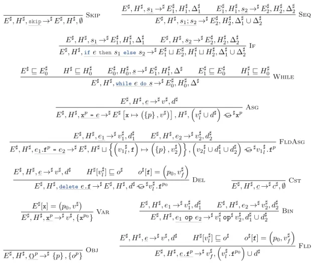
Figure 10 shows the rules of this analysis. To avoid burdening notations, we denote by d♯. f the⊂
abstract dependency relation{(fd, f )
fd∈ d♯}. Following the same scheme, we freely use the notation
l♯.fp to denote the set{p 0.fp
p0∈ l♯}. As an example, here is the rule for assignments:
E♯, H♯, e →♯v♯, d♯ E♯, H♯,xp =e →♯E♯[ x7→({p} , v♯)] , H♯, ( vl♯∪ d♯).⊂♯xp Asg
This rule expresses that when encountering an assignment, an over-approximation of all the possible locations in the form of an abstract value v♯ and of the dependencies d♯of the assigned expression e
is computed. The abstract environment is then updated by setting the variablexto this new abstract
value. Every possible flow from a potential dependency y ∈ d♯ or possible location value v♯l of the
expression e is marked as flowing intox. The position ofxis taken into account in the resulting flows.
The Bin rule makes use of an abstract operation op♯, which depends on the operators added in
the language. Figure 16 in Appendix B shows an example of analysis on the code we have seen on the previous sections, namelyx= {};x.f= {};if falsethen y=x.felse y= {}.
There are several possible variations and extensions of this analysis. For one notable example it could be refined with strong updates on locations. For the moment, we leave for further work how exactly to annotate the semantics and to abstract locations in order to state whether or not an abstract location represents a unique concrete location in the heap.
4.3.
Analysis in Coq
The abstract domains are essentially the same as the ones described in Section 4.1. They are straightforward to formalize as soon as basic constructions for lattices are available: the abstract domains are just specific instances of standard lattices from abstract interpretation (flat lattices,
E♯, H♯,skip→♯E♯, H♯, ∅ Skip E♯, H♯, s 1→♯E1♯, H ♯ 1, ∆ ♯ 1 E ♯ 1, H ♯ 1, s2→♯E2♯, H ♯ 2, ∆ ♯ 2 E♯, H♯, s 1; s2→♯E2♯, H ♯ 2, ∆ ♯ 1∪ ∆ ♯ 2 Seq E♯, H♯, s 1→♯E♯1, H ♯ 1, ∆ ♯ 1 E♯, H♯, s2→♯E2♯, H ♯ 2, ∆ ♯ 2 E♯, H♯,ifethens 1 elses2→♯E1♯⊔ E ♯ 2, H ♯ 1⊔ H ♯ 2, ∆ ♯ 1∪ ∆ ♯ 2 If E♯⊑ E♯ 0 H♯⊑ H ♯ 0 E ♯ 0, H ♯ 0, s→♯E ♯ 1, H ♯ 1, ∆♯ E ♯ 1⊑ E ♯ 0 H ♯ 1⊑ H ♯ 0 E♯, H♯,whileedos →♯E♯ 0, H ♯ 0, ∆♯ While E♯, H♯, e →♯v♯, d♯ E♯, H♯,xp =e →♯E♯[x7→({p} , v♯)] , H♯,(vl♯∪ d♯).⊂♯xp Asg E♯, H♯, e1→♯v♯1, d ♯ 1 E♯, H♯, e2→♯v♯2, d ♯ 2 E♯, H♯, e1.fp = e2→♯E♯, H♯⊔ {( v1♯l,f ) 7→({p} , v♯2 )} ,(v2♯l∪ d♯1∪ d ♯ 2 ) ⊂ . ♯v 1♯l.fp FldAsg E♯, H♯, e→♯v♯, d♯ H♯[v♯ l] ⊑ o ♯ o♯[f] =(p 0, vf♯ ) E♯, H♯,deletee.f→♯E♯, H♯, d♯.⊂♯vl♯.fp0 Del E♯, H♯, c →♯c♯, ∅ Cst E♯[x] =(p 0, v♯) E♯, H♯,xp→♯v♯, {xp0} Var E ♯, H♯, e 1→♯v1♯, d ♯ 1 E♯, H♯, e2→♯v2♯, d ♯ 2 E♯, H♯, e 1ope2→♯v1♯op♯v ♯ 2, d ♯ 1∪ d ♯ 2 Bin E♯, H♯,{}p→♯ {p} , {op} Obj E♯, H♯, e →♯v♯, d♯ H♯[v♯l] ⊑ o♯ o♯[f] = ( p0, v♯f ) E♯, H♯, e.fp→♯v♯f, ( vl♯.fp0) ∪ d♯ Fld
Figure 10: Rules for the Abstract Reduction Relation
power set lattices. . . ). For the certification of lattices we refer to the Coq developments by David Pichardie [10].
Similarly to Section 3.6, the rules of the analyzer presented in Figure 10 are first defined as an inductive predicate of type
t AEnvironment→t AHeap→stat→t AEnvironment→t AHeap→t AFlows→Prop
where the two typest AEnvironmentandt AHeapare the types of the abstract lattices for environments and heaps, and t AFlows the type of abstract flows, represented as a lattice for convenience. The analyzer is then defined by an extractable function of similar type (excepting the final “→Prop”), the
two definitions being proven equivalent. The situation for expressions is similar.
Once the analysis has been defined as well as the instrumentation, it’s possible to formally prove the correctness of the abstract reduction rules with respect to the instrumentation. The property to prove is the one shown in Section 4.2: if from an empty heap, a program reduces to a heap Eτ, Hτ and
flows ∆τ, then if from the ⊥ abstraction, a program reduces to E♯, H♯ and abstract flows ∆♯; that
is, [] , ∅, [], ∅, ∅, s→ τ, Mτ, ∆τ, Eτ, Hτ and⊥, ⊥, s →♯E♯, H♯, ∆♯, then E ≺ E♯, H ≺ H♯and ∆τ ≺ ∆♯.
5.
Conclusion
Schmidt’s natural semantics-based abstract interpretation is a rich framework which can be instantiated in a number of ways. In this paper, we have shown how the framework can be applied to the particular style of natural semantics called pretty big step semantics. We have studied a particular kind of intentional information about the program execution, viz., how information flows from points of creation to points of use. This has lead us to define a particular abstraction of semantic derivation trees for describing points in the execution. This abstraction can then be further combined with other abstractions to obtain an abstract reduction relation that formalizes the static analysis.
Other systematic derivation of static analyses have taken small-step operational semantics as starting point. Cousot [4] has shown how to systematically derive static analyses for an imperative language using the principles of abstract interpretation. Midtgaard and Jensen [8, 9] used a similar approach for calculating control-flow analyses for functional languages from operational semantics in the form of abstract machines. Van Horn and Might [14] show how a series of analyses for functional languages can be derived from abstract machines. An advantage of using small-step semantics is that the abstract interpretation theory is conceptually simpler and more developed than its big-step counterpart. Our motivation for developing the big-big-step approach further is that the semantic framework has certain modularity properties that makes it a popular choice for formalizing real-sized programming languages.
Our preliminary experiments show that the semantics and its abstractions lend themselves well to being implemented in the Coq proof assistant. This is an important point, as some form of mechanization is required to evaluate the scalability of the method. Scalability is indeed one of the goals for this work. The present paper establishes the principles with which we hope to achieve the generation of an analysis for full JavaScript based on its Coq formalization. However, this will require some form of machine-assistance in the production of the abstract semantics. The present work provides a first experience of how to proceed. Further work will now have to extract the essence of this process and investigate how to program it in Coq.
One this has been achieved, we will be well armed to attack other analyses. One immediate candidate for further work is full information flow analysis, taking indirect flows due to conditionals into account. It would in particular be interesting to see if the resulting abstract semantics can be used for a rational reconstruction of the semantic foundations underlying the dynamic and hybrid information flow analysis techniques developed by Le Guernic, Banerjee, Schmidt and Jensen [7]. Combined with the extension to full JavaScript, this would provide a certified version of the recent information flow control mechanisms for JavaScript such as the monitor proposed by Hedin and Sabelfeld [6].
Bibliographie
[1] M. Bodin, A. Charguéraud, D. Filaretti, P. Gardner, S. Maffeis, D. Naudziuniene, A. Schmitt, and G. Smith. Jscert: Certified javascript. http://jscert.org/, 2012.
[2] M. Bodin, T. Jensen, and A. Schmitt. Pretty-big-step certified abstract interpretation, coq source code. http://www.irisa.fr/celtique/aschmitt/research/owhileflows/, 2013.
[3] A. Charguéraud. Pretty-big-step semantics. In ESOP 2013, pages 41–60. Springer, 2013. [4] P. Cousot. The calculational design of a generic abstract interpreter. In Calculational System
Design. NATO ASI Series F. IOS Press, Amsterdam, 1999.
[5] S. Guarnieri, M. Pistoia, O. Tripp, J. Dolby, S. Teilhet, and R. Berg. Saving the world wide web from vulnerable javascript. In ISSTA 2011, pages 177–187. ACM Press, 2011.
[6] D. Hedin and A. Sabelfeld. Information-flow security for a core of javascript. In Proc. of the 25th Computer Security Foundations Symp. (CSF’12), pages 3–18. IEEE, 2012.
[7] G. Le Guernic, A. Banerjee, T. Jensen, and D. Schmidt. Automata-based Confidentiality Monitoring. In ASIAN 2006, pages 75–89. Springer LNCS vol. 4435, 2006.
[8] J. Midtgaard and T. Jensen. A calculational approach to control-flow analysis by abstract interpretation. In SAS 2008, volume 5079 of LNCS, pages 347–362. Springer Verlag, 2008. [9] J. Midtgaard and T. Jensen. Control-flow analysis of function calls and returns by abstract
interpretation. In ICFP 2009, pages 287–298. ACM, 2009.
[10] D. Pichardie. Building certified static analysers by modular construction of well-founded lattices. In FICS 2008, volume 212 of ENTCS, pages 225–239, 2008.
[11] D. Schmidt. Natural-semantics-based abstract interpretation (preliminary version). In Proc. 2d Static Analysis Symposium (SAS’95), pages 1–18. Springer LNCS vol. 983, 1995.
[12] E. Schwartz, T. Avgerinos, and D. Brumley. All you ever wanted to know about dynamic taint analysis and forward symbolic execution (but might have been afraid to ask). In S&P, 2010. [13] D. L. M. Valérie Gouranton. Dynamic slicing: a generic analysis based on a natural semantics
format. Journal of Logic and Computation, 9(6), 1999.
[14] D. Van Horn and M. Might. Abstracting abstract machines. In ICFP, pages 51–62. ACM, 2010. [15] P. Vogt, F. Nentwich, N. Jovanovic, E. Kirda, C. Kruegel, and G. Vigna. Cross-site scripting
A.
Traces and Program Points
In this section we define how to add program points to programs, in order to identify syntactic positions in the program, and we show how to relate traces from a semantic derivation with program points.
A.1.
Program Points
Program points are defined as chains of atoms. The transformation Π described below takes a program point and a term, and annotates each sub-term with program points before and after the sub-term. The program point before a syntactic construct is a context, a chain of atoms indicating where to find the term in the initial program. The program point after is a context followed by the atom identifying the syntactic construct corresponding to the sub-term. For instance, the program point Seq2/Seq2/IfE refers to the point before false in the term x= {};x.f= {};if false theny= x.felsey = {}; and
Seq2/Seq2/IfE/Cst to the point after. The notion of “before” and “after” a program point is standard in data flow analysis, but is here given a semantics-based definition.
We write· for the empty program point, and we assume program points have a monoid structure, with / as concatenation and · as neutral element.
Π(PP,skip) = PP,skip, PP/Skip
Π(PP, s1; s2) = PP, Π(PP/Seq1, s1); Π(PP/Seq2, s2), PP/Seq
Π(PP,ifethens1 elses2) = PP,ifΠ(PP/IfE, e) thenΠ(PP/IfT, s1)elseΠ(PP/IfF, s2), PP/If
Π(PP,whileedos) = PP,whileΠ(PP/WhileE, e)doΠ(PP/WhileS, s), PP/While Π(PP,x=e) = PP,x=Π(PP/AsgE, e), PP/Asg
Π(PP, e1.f=e2) = PP, Π(PP/FldAsgL, e1).f= Π(PP/FldAsgV, e2), PP/FldAsg
Π(PP,deletee.f) = PP,deleteΠ(PP/DelE, e).f, PP/Del
Π(PP, c) = PP, c, PP/Cst Π(PP,x) = PP,x, PP/Var
Π(PP, e1 ope2) = PP, Π(PP/BinL, e1) op Π(PP/BinR, e2), PP/Bin
Π(PP,{}) = PP,{}, PP/Obj
Π(PP, e.f) = PP, Π(PP/FldE, e).f, PP/Fld
To derive program points from traces, we first need to define an operator that deletes atoms in a chain up to a given atom. More precisely, the operator PP↓Name removes the shortest suffix of PP
that starts with Name, included. Formally, it is defined as follows.
· ↓Name = ·
PP/Name ↓Name = PP
PP/Name’ ↓Name = PP ↓Name if Name’̸= Name
A.2.
Traces
We give in Figure 11 the names that are added to the trace for each rule, following the general annotation scheme of Section 3.2. In the next step, the annotation of the left of the current rule is ignored, only the annotation on the right of the first premise is used.
Rule axiom up next down
Skip Skip
Seq Seq1 Seq1 Seq
Seq1 Seq2 Seq2
If IfE IfE If
IfTrue IfT IfT
IfFalse IfF IfF
While WhE WhE While
WhileTrue1 WhS WhS WhT1
WhileTrue2 WhL WhT2
WhileFalse WhF
Asg AsgE Asge Asg
Asg1 Asg1
FldAsg FldAsgL FldAsgL FldAsg
FldAsg1 FldAsgV FldAsgV FldAsg1
FldAsg2 FldAsg2
Del DelE DelE Del
Del1 Del1
Cst Cst
Var Var
Bin BinL BinL Bin
Bin1 BinR BinR Bin1
Bin2 Bin2
Obj Obj
Fld FldE FldE Fld
Fld1 Fld1
Abort Abort
Figure 11: Traces Definition
A.3.
From Traces to Program Points
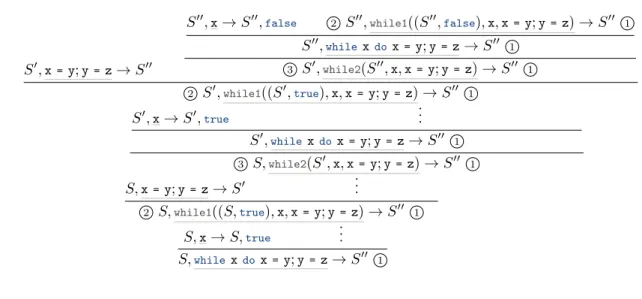
We next define a function T from traces to program points. There are two challenges in doing so. First, traces mention everything that has happened up to the point under consideration. Program points, however, hide everything that is not under the current execution context. We take care of this folding using the deletion operator defined above. The second challenge is to decide what program point to assign for extended statements and expressions, and when to decide that a statement has finished executing. To illustrate this challenge, we consider the case of a while loop, where in the initial environment we havex andyequal totrue and z equal tofalse.
The evaluation of the variablexonly adds Var at the end of the trace. The evaluation of the two
assignments appends the following sequence to the trace, which we call τs in the following.
S,x→ S,true S,x=y;y=z→ S′
S′,x→ S′,true
S′,x= y;y= z→ S′′
S′′,x→ S′′,false 2.. S′′,while1((S′′,false),x,x=y;y=z) → S′′ 1..
S′′,whilexdox=y;y= z→ S′′ 1.. .. 3 S′,while2(S′′,x,x=y;y=z) → S′′ 1.. .. 2 S′,while1((S′,true),x,x=y;y= z) → S′′ 1.. ·· · S′,whilexdox=y;y=z→ S′′ 1.. .. 3 S,while2(S′,x,x=y;y=z) → S′′ 1.. ·· · .. 2 S,while1((S,true),x,x=y;y=z) → S′′ 1.. ·· · S,whilexdox=y;y=z→ S′′ 1..
Figure 12: Running a While loop
The whole trace at the end of the execution has the following form. [WhE; Var; WhE; WhS] ++ τs++ [WhS; WhL] ++
[WhE; Var; WhE; WhS] ++ τs++ [WhS; WhL] ++
[WhE; Var; WhE; WhF] ++
[While; WhT2; WhT1; While; WhT2; WhT1; While] The program point on the right-hand-side of every→ S′′ should be While ( ..1), as it corresponds
to the end of the program. The program point before everywhile1( ..2) should be the same on as right
after evaluating the condition, namely WhileE/Var. Similarly, the one beforewhile2( ..3) is taken to
be the one right after finishing to evaluate the sequence, namelyWhileS/Seq.
Following this intuition, we define in Figure 13 the T function that takes a trace and an already computed program point, then creates a program point. A quasi invariant is that part of a program point is deleted only if a new atom is added, reflecting the notion that evaluation never goes back in the program syntax. There is a crucial exception, though: when doing a loop for awhileloop (premise of rule While2), then the program point jumps back to right before the while loop.
We now state that program points can correctly be extracted from traces. To this end, we consider a derivation where the terms contain program points.
Property 4 Let t be a term and t′ = Π(·, t). For any occurrence of a rule the form τ, S, PP, t, PP′→
T ([], PP) = PP
T (Skip :: τ, PP) = T (τ, PP/Skip)
T (Seq1 :: τ, PP) = T (τ, PP/Seq1) T (Seq1 :: τ, PP) = T (τ, PP) T (τ, PP/Seq) = T (τ, PP)
T (Seq2 :: τ, PP) = T (τ, PP ↓Seq1/Seq2) T (Seq2 :: τ, PP) = T (τ, PP ↓Seq2/Seq)
T (IfE :: τ, PP) = T (τ, PP/IfE) T (IfE :: τ, PP) = T (τ, PP) T (If :: τ, PP) = T (τ, PP)
T (IfT :: τ, PP) = T (τ, PP ↓IfE/IfT) T (IfT :: τ, PP) = T (τ, PP ↓IfT/If)
T (IfF :: τ, PP) = T (τ, PP ↓IfE/IfF) T (IfF :: τ, PP) = T (τ, PP ↓IfF/If)
T (WhE :: τ, PP) = T (τ, PP/WhE) T (WhE :: τ, PP) = T (τ, PP) T (While :: τ, PP) = T (τ, PP) T (WhS :: τ, PP) = T (τ, PP ↓WhE/WhS) T (WhS :: τ, PP) = T (τ, PP) T (WhT1 :: τ, PP) = T (τ, PP) T (WhL :: τ, PP) = T (τ, PP ↓WhS) T (WhT2 :: τ, PP) = T (τ, PP) T (WhF :: τ, PP) = T (τ, PP/While)
T (AsgE :: τ, PP) = T (τ, PP/Asge) T (AsgE :: τ, PP) = T (τ, PP) T (Asg :: τ, PP) = T (τ, PP)
T (Asg1 :: τ, PP) = T (τ, PP ↓AsgE/Asg)
T (FldAsgL :: τ, PP) = T (τ, PP/FldAsgL) T (FldAsgL :: τ, PP) = T (τ, PP) T (FldAsg :: τ, PP) = T (τ, PP)
T (FldAsgV :: τ, PP) = T (τ, PP ↓FldAsgL/FldAsgV) T (FldAsgV :: τ, PP) = T (τ, PP)
T (FldAsg1 :: τ, PP) = T (τ, PP)
T (FldAsg2 :: τ, PP) = T (τ, PP ↓FldAsgV/FldAsg)
T (DelE :: τ, PP) = T (τ, PP/DelE) T (DelE :: τ, PP) = T (τ, PP) T (Del :: τ, PP) = T (τ, PP)
T (Del1 :: τ, PP) = T (τ, PP ↓DelE/Del)
T (Cst :: τ, PP) = T (τ, PP/Cst) T (Var :: τ, PP) = T (τ, PP/Var)
T (BinL :: τ, PP) = T (τ, PP/BinL) T (BinL :: τ, PP) = T (τ, PP) T (Bin :: τ, PP) = T (τ, PP)
T (BinR :: τ, PP) = T (τ, PP ↓BinL/BinR) T (BinR :: τ, PP) = T (τ, PP)
T (Bin1 :: τ, PP) = T (τ, PP)
T (Bin2 :: τ, PP) = T (τ, PP ↓BinR/Bin)
T (Obj :: τ, PP) = T (τ, PP/Obj)
T (FldE :: τ, PP) = T (τ, PP/FldE) T (FldE :: τ, PP) = T (τ, PP) T (Fld :: τ, PP) = T (τ, PP)
T (Fld1 :: τ, PP) = T (τ, PP ↓FldE/Fld)
B.
Derivation examples
Asg Obj H[l] = ⊥ H ′= H[l 7→{}] E, H,{}→ E, H′, l E′= E[x7→ l] E, H,x =1E, H′, l → E′, H′ Asg1 E, H,x= {}→ E′, H′ FldAsg Var E ′[x] = l E′, H′,x→ E′, H′, l Obj H′[l′] = ⊥ H′′= H′[l′ 7→{}] E′, H′,{}→ E′, H′′, l′ H′[l] ={} o′={f7→ l′} H′′′= H′′[l 7→ o′] E′, H′, l.f = 2(E′, H′′, l′) → E′, H′′′ FldAsg2 E′, H′, (E′, H′, l).f = 1{}→ E′, H′′′ FldAsg1 ·· ·· ·· ·· E′, H′,x.f= {}→ E′, H′′′ Cst E′, H′′′,false→ E′, H′′′,false Obj H ′′′[l′′] = ⊥ H f = H′′′[l′′7→{}] E′, H′′′,{}→ E′, H f, l′′ Ef = E′[x7→ l′′] E′, H′′′,x = 1(E′, Hf, l′′) → Ef, Hf Asg1 E′, H′′′,y= {}→ E f, Hf Asg E′, H′′′,if1(E′, H′′′,false,y=x.f,y= {}) → E f, Hf IfFalse ·· ·· ·· E′, H′′′,if falsetheny =x.felse y= {}→ Ef, Hf
If
E′, H′, (E′, H′′′) ;
1if falsetheny= x.felse y= {}→ Ef, Hf
Seq1 ·· ·· ·· ·· ·· ·· ·· ·· ·· ·· ·· ·· ·· ·· ·· ·· · E′, H′,x.f= {};if falsethen y=x.felsey= {}→ E
f, Hf
Seq
E, H, (E′, H′) ;
1x.f= {};if false theny=x.felsey= {}→ Ef, Hf
Seq1 ·· ·· ·· ·· ·· ·· · E, H,x= {};x.f= {};if false theny=x.felsey= {}→ Ef, Hf
Seq
Asg Cst E, H,true→ E, H,true E′ = E[x7→true] E, H,x =1(E, H,true) → E′, H Asg1 E, H,x= true→ E′, H Var E ′[x] =true E′, H, x → E′, H,true E′′= E′[y7→true] E′, H,x = 1E′, H,true→ E′′, H Asg1 E′, H,y=x→ E′′, H Asg E, H, (E′, H) ; 1y=x→ E′′, H Seq1 ·· ·· ·· ·· ·· · E, H,x=true;y= x→ E′′, H Seq
(a) Unannotated Derivation
τ1= [] τ2= [Seq1] τ3= τ2++ [AsgE] τ4= τ3++ [Cst] τ5= τ4++ [AsgE]
τ6= τ5++ [Asg1] τ7= τ6++ [Asg] τ8= τ7++ [Seq1] τ9= τ8++ [Seq2] τ10= τ9++ [AsgE]
τ11= τ10++ [Var] τ12= τ11++ [AsgE] τ13= τ12++ [Asg1] τ14= τ13++ [Asg]
τ15= τ14++ [Seq2] τ16= τ15++ [Seq] Asg Cst τ3, E, H,true→τ4, E, H,true E′= E[x 7→true] τ5, E, H, x =1(E, H,true) → τ6, E′, H Asg1 τ2, E, H, x=true→τ7, E′, H Var E ′[x] =true τ10, E′, H, x → τ11, E′, H,true E′′= E′[y 7→true] τ12, E′, H, x =1E′, H,true→τ13, E′′, H Asg1 τ9, E′, H, y=x → τ14, E′′, H Asg τ8, E, H,(E′, H) ;1y=x → τ15, E′′, H Seq1 · · · · · · · · · · · τ1, E, H, x=true; y=x → τ16, E′′, H Seq
(b) Derivation Annotated With Traces
E♯1= {x7→ ({p1} , {p2})} E2♯= {x7→ ({p1} , {p2}) ,y7→ ({p6} , {p5})} E3♯= {x7→ ({p1} , {p2}) ,y7→ ({p9} , {p10})} E4♯= {x7→ ({p1} , {p2}) ,y7→ ({p6, p9} , {p5, p10})} H1♯= {(p2,f) 7→ ({p4} , {p5})} Asg Obj ⊥, ⊥,{}p2 →♯ {p 2} , {op2} ⊥, ⊥,xp1 = {}p2 →♯E♯ 1, ⊥, {op 2 ⊂ . xp1 } FldAsg Var E ♯ 1[x] = ({p1} , {p2}) E1♯, ⊥,x p3 →♯{p2} , {xp1} E1♯, ⊥,{} p5 →♯ {p5} , {op5} Obj E1♯, ⊥,x p3 .fp4 = {}p5 →♯E1♯, H ♯ 1, {{x p1 , op5 } ⊂. op2 .fp4 } Asg Fld Var E ♯ 1[x] = ({p1} , {p2}) E♯1, H ♯ 1,xp 7→♯ {p 2} , {xp1} H1♯[{op 2}] [ f] = ({p4} , {p5}) E1♯, H ♯ 1,xp 7 .fp8→♯{p 5} , {op2.fp8,xp1} E1♯, H ♯ 1,yp 6 = x.f→♯E♯2, H ♯ 1, {{op 5 , op2 .fp8 ,xp1} ⊂ . yp6} ·· ·· ·· ·· E1♯, H ♯ 1,{}p 10→♯ {p 10} , {op10} Obj E1♯, H ♯ 1,yp 9 = {}→♯E3♯, H1♯, {op10.⊂ yp9} Asg E1♯, H ♯
1,if falsetheny= x.felse y= {}→ ♯E♯ 4, H ♯ 1, {{o p5 , op2 .fp8 ,xp1 } ⊂. yp6 , op10 ⊂ . yp9 } If ·· ·· ·· ·· ·· ·· · E1♯, ⊥,x.f= {};if false theny= x.felsey= {}→
♯E♯ 4, H ♯ 1, {{x p1 , op5 } ⊂. op2 .fp4 , {op5 , op2 .fp8 ,xp1 } ⊂. yp6 , op10 ⊂ . yp9 } Seq ·· ·· ·· ·· ·· · ⊥, ⊥,x= {}p2; x.f= {}p5;
if false theny= x.felsey= {}p10→♯E♯
4, H ♯ 1, {op2 ⊂ . xp1 , {xp1 , op5 } ⊂. op2 .fp4 , {op5, op2 .fp8, xp1} ⊂. yp6, op10.⊂ yp9 } Seq