HAL Id: hal-01368466
https://hal-ensta-bretagne.archives-ouvertes.fr/hal-01368466
Submitted on 6 Nov 2017
HAL is a multi-disciplinary open access
archive for the deposit and dissemination of
sci-entific research documents, whether they are
pub-lished or not. The documents may come from
teaching and research institutions in France or
abroad, or from public or private research centers.
L’archive ouverte pluridisciplinaire HAL, est
destinée au dépôt et à la diffusion de documents
scientifiques de niveau recherche, publiés ou non,
émanant des établissements d’enseignement et de
recherche français ou étrangers, des laboratoires
publics ou privés.
A Modeling and Control approach for a cubic AUV
Benoit Clement, Yang Rui, Ali Mansour, Li Ming
To cite this version:
Benoit Clement, Yang Rui, Ali Mansour, Li Ming. A Modeling and Control approach for a cubic AUV.
10th IFAC Conference on Control Applications in Marine Systems, Sep 2016, Tronheim, Norway.
pp.279 - 284, �10.1016/j.ifacol.2016.10.355�. �hal-01368466�
A Modeling and Control approach for a
cubic AUV
Benoit Clement∗ Yang Rui∗∗ Ali Mansour∗ Li Ming∗∗
∗Lab-STICC, UMR CNRS 6285, ENSTA Bretagne, 29806 Brest Cedex
9, France (e-mail: [email protected]).
∗∗Ocean University of China, College of Engineering, Qingdao 266100,
China (e-mail: [email protected])
Abstract: This paper presents a control synthesis methodology for a cubic AUV. The modeling
part is based on CFD calculation and the control part is based on H∞ theory, nonlinear
compensation, Smith compensation and Kalman filter. It is presented and adapted to Ciscrea AUV for heading control. A comparison with PID controller is given with simulations and sea tests.
Keywords: Robust Control, AUV, application, modelling 1. INTRODUCTION
Underwater vehicles have a large variety of types and they are widely involved in undersea surveillance, inspection and survey missions (Clement (2013b)). Typically, AUVs and gliders are common with a torpedo shape for long range missions, and Human Occupied Vehicles (HOVs) as well as Remote Operating Vehicles (ROVs) are generally of a cubic shape used for hovering tasks. Note that, for some specific applications: undersea pipeline inspection, offshore infrastructure surveillance and large vessel maintenance, a small size cubic AUV is preferred. Indeed, small AUVs can be deployed to explore areas which are not accessible to HOVs and ROVs. Meanwhile, the cubic shaped AUVs enjoy more degrees of freedom than torpedo-shaped AUVs. Indeed, they can hover and enter complex underwater spaces.
Achieving good maneuverability of small AUV depends on two key factors: an accurate hydrodynamic model and an advanced control system. Yamamoto (Aug., 2001) pointed out that a model-based control system is more efficient if the dynamics of the vehicle are modeled to some extent. Meanwhile, Ferreira et al. (April, 2012) show that an empirical linear model often fails to represent the dynamics of the AUV over a wide operating region. In this work, we adopt our previously published model (Yang et al. (2015)). Regardless of modeling issues, the value of a model-based control approach depends on how robust and efficient the control scheme can adopt the hydrodynamic model. Poten-tial trends of current methods focus on faster controllers to assist the pilot or the autopilot with better accuracy. Op-timal controllers can reduce propelling actions to save the battery power as well as to increase the propeller lifespan. Moreover, numerous uncertainties should be considered, including parameter variations, nonlinear hydrodynamic damping effects, sensor transmit delays and ocean current disturbances. In robotic competitions (SAUC-E and eu-Rathlon), it has been shown that a PID yaw controller was less efficient for a low mass AUV. Consequently, advanced
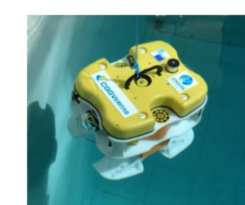
Fig. 1. CISCREA AUV picture in the test pool of ENSTA Bretagne
Table 1. CISCREA AUV main characteristics
Size 0.525m (L) 0.406m (W) 0.395m (H)
Weight in air 15.56 kg (without payload and floats)
Degrees of Freedom Surge, Sway, Heave and Yaw
Propulsion 2 vertical and 4 horizontal propellers
Speed 2 knots (Surge) & 1 knot (Sway, Heave)
Depth Rating 50m
On-board Battery 2-4 hours
control algorithms should be involved, such as the adaptive control scheme by Maalouf et al. (Feb., 2013), interval analysis approach by Jaulin and Le Bars (2012). Note that robust control schemes are shown to be successfully by Feng and Allen (Feb., 2004) and Roche et al. (pp. 17-24, Sep., 2010) for torpedo-shaped AUVs. In this work, we appointed the CISCREA AUV shown in Figure 1 and main characteristics are given in Table 1.
This work is organized as follows. AUV main notions, Ciscrea model and its derivative equations for control design are presented in Section 2. A control scheme based
on nonlinear feedback and H∞optimization is proposed in
Section 3. Section 4 shows the Matlab simulation results
of H∞ and PID controllers. In addition, the improved
H∞ scheme adaption and sea tests are presented. It is
simulation to real envirionment like it has been done for other robots (Clement (2013a)).
In this paper, we propose a original embedded control structure simple model oriented; using Kalman filters, the unmeasured and noisy system states are estimated. A Smith compensator is introduced to compensate the magnetic compass delay. The system uncertainties are
dealt with H∞ theory. The experiment and simulation
results show the advantages of the proposed CFD model based H-infinity methods compared with PID controller.
2. AUV MODELING
This section is dedicated to describe the AUV modeling notions as well as the dynamic and hydrodynamic parame-ters of Ciscrea AUV. A yaw model is derived in this section for robust heading control design. Note that, modeling data in this section comes from our previous CFD works (Yang et al. (2015)).
2.1 AUV Modeling Notions
Ciscrea AUV dynamics are represented marine vehicle formulation by Fossen (2002) and by the Society of Naval Architects and Marine Engineers (SNAME (April 1950)). Positions, angles, linear and angular velocities, force and moment definitions are reflected in Tab 2. The position vector η, velocity vector ν and force vector τ are defined as follows:
η = [x, y, z, φ, θ, ψ]T;
ν = [u, v, w, p, q, r]T ;
τ = [X, Y, Z, K, M, N ]T
Table 2. The notation of SNAME Positions and
Angles
Velocities Forces and
Moments
Coordinate NED-frame B-frame B-frame
Surge x u X Sway y v Y Heave z w Z Roll φ p K Pitch θ q M Yaw ψ r N
According to Fossen (2002), rigid-body hydrodynamic forces and moments can be linearly superimposed. There-fore, the overall non-linear underwater model can be char-acterized by two parts, the rigid-body dynamic (1) and hydrodynamic formulations (2) (hydrostatics included):
MRBν + C˙ RB(ν)ν = τenv+ τhydro+ τpro (1)
τhydro = −MAν − C˙ A(ν)ν − D(|ν|)ν − g(η) (2)
Table 3 describes the parameters of this model. Due to the size of the matrices and the figures needed to show all the numerical values, the reader can refear to the paper dedicaded to modeling (Yang et al. (2015)).
For the Ciscrea AUV, the rigid-body mass inertia
ma-trix MRB is simplified due to symmetry. Here, rG =
[xG, yG, zG]T is the vector from Ob (origin of B-frame) to
CG (center of gravity).
CRB and CA contribute to the centrifugal force. Note
that a practical way to calculate these two matrices using
Table 3. Nomenclature of the notations
Parameter Description
MRB AUV rigid-body mass and inertia matrix
MA Added mass matrix
CRB Rigid-body induced coriolis-centripetal matrix
CA Added mass induced coriolis-centripetal matrix
D(|v|) Damping matrix
g(η) Restoring forces and moments vector
τenv Environmental disturbances (wind, waves and
cur-rents)
τhydro Vector of hydrodynamic forces and moments
τpro Propeller forces and moments vector
MRB, MAand ν is introduced in Marine System Simulator
(MSS (2010)). In our case, these two matrices can be neglected due to the low speed to be considered, C(v) ≈ 0. For an AUV with neutral buoyancy, the weight W is approximately equal to the buoyancy force B.
For Ciscrea AUV, CB (the buoyancy center) and CG are located using trials and errors method by adding and removing the payload and floats. The marine disturbances, such as the wind, waves and currents are related to the
environmental effect τenv. However for a deep sea
un-derwater vehicle, only current should be considered since wind and waves have negligible effects. Two
hydrody-namic parameters added mass, MA∈ R6×6, and damping,
D(|ν|) ∈ R6×6, should be carefully involved in the AUV
model. Added mass is a virtual conception representing the hydrodynamic forces and moments. Any accelerating
emerged-object would encounter this MAdue to the inertia
of the fluid. For a cubic-shaped AUV, added mass in some directions are generally larger than the rigid-body mass as explained by Yang et al. (May, 2014). Damping in the
fluid consists of four parts: Potential damping DP(|ν|),
skin friction DS(|ν|), wave drift damping DW(|ν|) and
vor-tex shedding damping DM(|ν|). For the CISCREA AUV,
quadratic damping is the main dynamic nonlinearity of the system (Yang et al. (May, 2014)).
2.2 Ciscrea model
For applying the methodology to the Ciscrea AUV, Mass
inertia matrix, MRB, is calculated using PRO/ENGINEER
software, and added mass matrix, MA, is calculated
us-ing WAMITTM based on radiation/diffraction program.
Finally, STAR-CCM+TM software and real world
experi-ments are conducted to estimate the relationship among damping forces, damping moments, vehicle velocities and angular velocities. In Yang et al. (May, 2014, 2015), second order polynomial lines are implemented to approximate the relationship between damping and velocities.
2.3 Yaw model
Without loss of generality, we only present the robust con-troller in yaw direction. The rotational model is simplified as in (3) (neglecting buoyancy and gravity). Definitions and parametric values, such as inertia and damping coef-ficients, are listed in Table 4. Note that, all the param-eters have uncertainties, as they are either measured or numerically calculated. The uncertainties will be carefully
discussed and treated using H∞ solution in section 3.
Table 4. Rotational model parameters for yaw direction
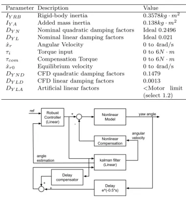
Parameter Description Value
IY RB Rigid-body inertia 0.3578kg · m2
IY A Added mass inertia 0.138kg · m2
DY N Nominal quadratic damping factors Ideal 0.2496
DY L Nominal linear damping factors Ideal 0.021
˙
xr Angular Velocity 0 to 4rad/s
τi Torque input 0 to 6N · m
τcom Compensation Torque 0 to 6N · m
˙
xr0 Equilibrium velocity 0 to 4rad/s
DY N D CFD quadratic damping factors 0.1479
DY LD CFD linear damping factors 0.0013
DY LA Artificial linear factors <Motor limit
(select 1.2) Nonlinear Model Robust Controller (Linear) Nonlinear Compensation + -ref kalman filter (Linear) yaw angle angular velocity Delay e^(-0.5*s) + + angle estimation Delay compensator
Fig. 2. Ciscrea H∞heading control scheme with nonlinear
and delay compensations, Kalman filter and linear
H∞controller.
3. CONTROL STRUCTURE
In this section, an original struture is proposed. It is based
on H∞ theory, nonlinear compensation, Smith
compensa-tion and Kalman filter. It is presented and adapted to Ciscrea AUV for heading control. The proposed structure is given on figure 2. One can see the various parts of the control.
We propose a framework to :
• change the nonlinear yaw model into a linear system with uncertainties based on previous modeling works (here is an important contribution that shows the links between control and modeling);
• tune a Kalman filter if only few sensors are used (compass in our case);
• tune a Smith compensator for the delay due to the low cost sensor;
• solve a H∞ controller for the linear system.
3.1 Nonlinear compensation
In this part, we discuss the nonlinear problem without concern of parametric uncertainties, such as inertia and damping coefficient errors. As shown in Yang et al. (May, 2014), damping is a major nonlinear component in the AUV model. Therefore, in Figure 3, we propose to com-pensate nonlinear behaviors using the CFD yaw model, as feedback for real world propellers.
The nonlinear compensation is given in equation (4).
τcom= (DY LA− DY LD− DY N D| ˙xr|) ˙xr (4)
where:
Nonlinear Yaw Model
Nonlinear Compensator Linear system with uncertainties
Angle Torque Angular Velocity Nonlinear Compensation Propellers Robust Controller (Linear) + -ref + -Sensors
Fig. 3. Nonlinear Compensator allows linear synthesis
• DY LAis the artificial linear factor given in Tab 4.
• DY N D and DY LD are CFD damping estimations.
The linear model result of compensation is given in equa-tion (5).
(DY LA+ (DY N| ˙xr| − DY N D| ˙xr| + DY L− DY LD)) ˙xr
+(IY RB+ IY A)¨xr= τi
(5)
The term δ = DY N| ˙xr| − DY N D| ˙xr| + DY L− DY LD is
calculated as an uncertainty added to DY LA. Generally,
this δ is small comparing to DY LA. If we calculate δ using
that: ˙
xr∈ [−4, 4] rad/s; DY LA=1.8; DY N=0.2496;
DY L=0.021; DY N D=0.1479; DY LD=0.0013;
we can consider that DY LAis a nominal parameter which
has a dynamic uncertainty of 23.7%.
(IY RB+ IY A)¨xr+ (DY LA+ δ) ˙xr= τi
δ ∈ [−0.4265, 0.4265] (6)
At the end, the proposed model, equation (6), is a linear
system with uncertainties. Therefore, H∞ approach is
feasible for this model as it is proposed in figure 3.
3.2 Linear controller: H∞ synthesis
Let us consider the following classical state space repre-sentation of a linear time invariant (LTI) system:
"x˙ z y # = "A B 1 B2 C1 D11 D12 C2 D21 D22 # "x w u # (7)
where x ∈ Rn is the state vector, u ∈ Rm2 the control
input, y ∈ Rp1 system output, w ∈ Rm1the external input
vector, z ∈ Rp2the error vector. The robust design process
is to find a LTI feedback controller K, such that the closed-loop system remains stable and is able to achieve given performances in presence of uncertainties (Gu et al. (2005); Zhou and Doyle (1998)). Generally, cost functions
for finding K are represented by H∞norms of the
closed-loop transfer functions from w to z, as seen in equation (8). min Kstable Wp(I + GK)−1 We(I + GK)−1 WuK(I + GK)−1 ∞ < γ (8)
Here, K is the robust controller in Figure 4, and G is the linear nominal yaw model. The nominal model is derived from the linear fractional transformation (LFT) technique,
Linear Nominal Model (G) Angle ref + -We Robust Controller (K) Wu Wp e u
Fig. 4. H∞ synthesis structure: weighting functions,
nom-inal model, controller.
which separates uncertainties into an individual block (Gu et al. (2005)).
In H∞ theory, weighting functions are introduced for
set-ting control specifications. Generally, it is difficult to get the accurate frequency characteristics of external input signals. Therefore, weighting functions are sometimes the upper bound that covers original signals. For example,
the weighting function Wp, which represents the frequency
characteristics of the external disturbance, is used to de-scribe output disturbance rejection ability. Satisfying the above norm inequality indicates that the closed-loop sys-tem indeed reduces the disturbance effects to a prescribed level.
Finding appropriate weighting functions is critical and difficult, trials are necessary for a successful robust control design. In this application, we choose a structure with three weighting functions as it can be seen in Figure 4.
We is chosen as a reference tracking error requirement,
Wu represents the input disturbance rejection. Wp, which
restricts the output disturbance, is the same specification
with We, but with different objectives.
Weighting function parameters are selected according to
equations (9) to (11). Wu is selected to be a very small
scalar (Gu = 0.01) for disturbance rejection. We choose
Weand Wpaccording to Gu et al. (2005) and Roche et al.
(pp. 17-24, Sep., 2010), carefully considered the robust margins, tracking error (1%) and fast response.
Wp(s) = 0.95 s2+ 1.8s + 10 s2+ 8s + 0.01 (9) We(s) = 0.5 s + 0.92 s + 0.0046 (10) Wu(s) = 0.01 (11)
To solve the H∞problem, one can use the Riccati method
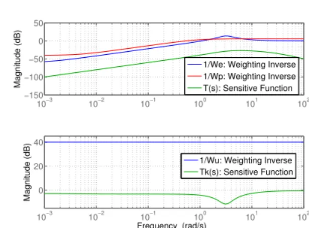
or Linear Matrix Inequality (LMI) approach Zhou and Doyle (1998). Usually, we prefer to choose the LMI ap-proach, as it requires less initial conditions (Gu et al. (2005)). The resulting transfers are given in Figure 5. 3.3 Delay compensation
First, underwater vehicles might not be equipped with enough sensors to detect all the states, such as the angular
velocity ˙xr. In addition, the magnetic compass may
en-counter serious signal delay and noise injection. Therefore, we propose to use a CFD model based kalman filters, numerically estimating unmeasured as well as noisy states. In addition, model based compensation algorithms are
10−3 10−2 10−1 100 101 102 −150 −100 −50 0 50 Magnitude (dB)
1/We: Weighting Inverse 1/Wp: Weighting Inverse T(s): Sensitive Function 10−3 10−2 10−1 100 101 102 0 20 40 Magnitude (dB) Frequency (rad/s)
1/Wu: Weighting Inverse Tk(s): Sensitive Function
Fig. 5. Sensitivity Functions and inverse of weighting functions 25 30 35 40 45 2 4 6 Angle (rad) Compass Desired Angle Kalman Estimation 25 30 35 40 45 −2 0 2 4 6 Torque (N*m) Hinf Thrust 25 30 35 40 45 −2 0 2 4 Time (second)
Anglular Velocity (rad/s)
Kalman Velocity Estimation
Fig. 6. Ciscrea H∞ heading control delay and noise
prob-lem
recommended to deal with the sensor delay. The proposed
H∞ approach is completed as it is shown in Figure 2.
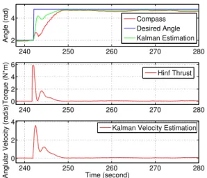
In order to reveal the magnetic compass delay as well as noise injections on the rotational motion of CISCREA
AUV, A less tuned H∞ heading controller was
demon-strated in Figure 6. Among the Kalman angle estimation and magnetic compass output, an obvious 0.5s delay was observed. In this case, the delay lead to distinct heading control oscillations. Meanwhile, there exist noise efforts on the control output to propellers.
For Ciscrea heading control application, a classical Smith compensator was introduced by Zhong (2006) to compen-sate the magnetic compass delay, see Figure 7 and equation (12).
P (s) = G0(s) − G0(s)e−0.5s (12)
The main idea is to estimate current delay free output y
from the nominal model G0(s) and real output ye(−0.5+δ)s.
Figure 8 shows the H∞heading control simulation results
Fig. 7. Smith Predictor struture for delay compensation 48 50 52 54 56 58 60 62 2 3 4 5 Angle (radian) Reference Compass Output Kalman Output Real Angle 48 50 52 54 56 58 60 62 −2 0 2 4 6 Time (second) Torque (N*m) Hinf Control Nonlinear Compensation
Fig. 8. Improved Ciscrea H∞ heading controller (Smith
Compensation) 48 50 52 54 56 58 60 62 2 3 4 5 Angle (radian) Reference Compass Output Kalman Output Real Angle 48 50 52 54 56 58 60 62 −2 0 2 4 6 Time (second) Torque (N*m) Hinf Control Nonlinear Compensation
Fig. 9. Improved Ciscrea H∞ heading controller (Kalman
Compensation)
In addition, as robust controller is insensitive to compensa-tion errors, we are enlighten to propose another compen-sation scheme using Kalman angular velocity estimation
( ˙xr), see equation (13).
y = P (s)u + ye(−0.5+δ)s, y = Kcx˙r+ ye(−0.5+δ)s, Kc > 0
(13)
A Kc= 0.57 was tuned which has an efficient
compensa-tion result in Figure 9.
4. SIMULATION AND EXPERIMENTS 4.1 Heading control simulation
In the simulation, IY RB+ IY Aand DY LA are considered
to be two varying parameters, which have respectively 30% and 40% (> 23.7%) of variations. In Figure 10,
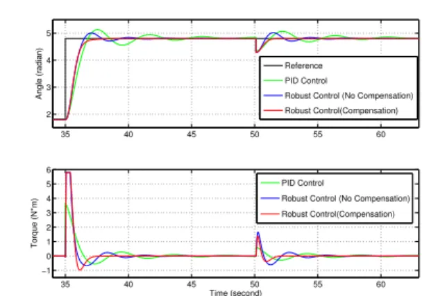
35 40 45 50 55 60 2 3 4 5 Angle (radian) Reference PID Control
Robust Control (No Compensation) Robust Control(Compensation) 35 40 45 50 55 60 −1 0 1 2 3 4 5 6 Time (second) Torque (N*m) PID Control
Robust Control (No Compensation) Robust Control(Compensation)
Fig. 10. Step Response and Propellor Output on Nominal Yaw Model 35 40 45 50 55 60 2 3 4 5 Angle (radian) Reference PID Control
Robust Control (No Compensation) Robust Control(Compensation) 35 40 45 50 55 60 −1 0 1 2 3 4 5 6 Time (second) Torque (N*m) PID Control
Robust Control (No Compensation) Robust Control(Compensation)
Fig. 11. Step Response and Propellor Output with 30% of interia variation
step responses of three scenarios are represented: PID
control, damping compensated H∞approach and bare H∞
control. From the simulation comparison, we can conclude
that compensated H∞controller handles the nonlinearity
with the fastest response. Compensated H∞controller has
no overshot and oscillations during the rotation process. Tracking error achieves the specification less than 1%. To emphasize the speed and robustness of our approach, we inject a small disturbance of 0.5rad on the output at 50s. Figure 11 shows the robust performance of our controller handling a yaw model with 30% inertia variations.
4.2 Ciscrea Sea Test
The proposed control scheme has been validated on Cis-crea in sea tests, and its results are compared with a traditional PID approach, respectively shown in Figures
12 and 13. First, H∞ heading controller is faster than
PID scheme (even with low battery conditions). Second, there is no nonlinearity induced oscillations in the control output, and the tracking accuracy is better. Third, from the propeller thrust signal, we can determine that the magnetic compass noise and disturbances are well rejected, while PID is less efficient to handle those uncertainties. Finally, the characteristics of our controller result in an optimal and smooth propulsion, which saves the battery energy, and allows to increase the working range.
240 250 260 270 280 2 4 Angle (rad) Compass Desired Angle Kalman Estimation 240 250 260 270 280 0 2 4 6 Torque (N*m) Hinf Thrust 240 250 260 270 280 0 2 4 Time (second)
Anglular Velocity (rad/s)
Kalman Velocity Estimation
Fig. 12. Ciscrea H∞ heading control sea experiment
(Kalman compensation) 90 100 110 120 130 140 150 2 3 4 5 time (second) Angle (rad) PID control Desired Angle 90 100 110 120 130 140 150 −1 0 1 2 Time (second) Torque (N*m) PID Thrust
Fig. 13. Ciscrea PID heading control sea experiment (Brest Port)
5. CONCLUSION
We have presented an efficient CFD model based H∞
control method to improve the motion performance of AUVs with uncertainties. It has been validated on the heading control scenario of low-mass and complex-shaped Ciscrea AUV in sea tests. Experimental and simulation
results have proved that CFD model based H∞has many
advantages comparing to PID controller: • faster in time response for a step demand;
• free from nonlinearity induced oscillations and over-shoot (CFD compensation);
• free from sensor delay induced oscillations (Delay compensation); efficient noise and disturbance
rejec-tion (Kalman filter and H∞perfomance constraints);
• not sensitive to parametric variation uncertainties (Robustness);
• optimal and smooth propulsion orders.
The proposed robust heading control application demon-strates a high quality AUV motion control solution, and finally it uses only one compass as feedback sensor.
ACKNOWLEDGEMENTS
This work was supported by the China Scholarship Coun-cil, Ocean University of China and ENSTA Bretagne.
REFERENCES
Clement, B. (2013a). Control algorithms for a sailboat
robot with a sea experiment. In Proceedings of the
9th IFAC Conference on Control Applications in Marine Systems. Osaka, Japan.
Clement, B. (2013b). A marine robotics point of view
for oceanography. In Innovation and Blue Growth
Symposium. Qingdao, China.
Feng, Z. and Allen, R. (Feb., 2004). Reduced order h∞
control of an autonomous underwater vehicle. Control Engineering Practice, 12(12), 1511–1520.
Ferreira, B.M., Matos, A.C., and Cruz, N.A. (April, 2012). Modeling and control of trimares auv. In 12th Interna-tional Conference on Autonomous Robot Systems and Competitions, 57–62. Portugal.
Fossen, T.I. (2002). Marine control systems: Guidance, navigation and control of ships, rigs and underwater vehicles. Marine Cybernetics Trondheim.
Gu, D.W., Petkov, P.H., and Konstantinov, M.M. (2005). Robust Control Design with MATLAB. Springer. Jaulin, L. and Le Bars, F. (2012). An interval approach
for stability analysis: Application to sailboat robotics. IEEE Transaction on Robotics,, 27(5), 282 – 287. Maalouf, D., Tamanaja, I., Campos, E., Chemori, A.,
Creuze, V., Torres, J., Rogelio, L., et al. (Feb., 2013). From pd to nonlinear adaptive depth-control of a teth-ered autonomous underwater vehicle. In 5th Symposium on System Structure and Control. Grenoble, France.
MSS (2010). Marine systems simulator
(2010) viewed 01.02.2014. [online]. available:
http://www.marinecontrol.org.
Roche, E., Sename, O., and Simon, D. (pp. 17-24, Sep.,
2010). Lpv/h∞ varying sampling control for
au-tonomous underwater vehicles. In 4th IFAC Symposium on System, Structure and Control. Delle Marche, Italy. SNAME (April 1950). Nomenclature for treating the
mo-tion of a submerged body through a fluid. The Society of Naval Architects and Marine Engineers, Technical and Reserach Bulletin, 1–15.
Yamamoto, I. (Aug., 2001). Robust and non-linear control of marine system. International Journal of Robust and Nonlinear Control, 11(13), 1285–1341.
Yang, R., Clement, B., Mansour, A., Li, H., Li, M.,
and Wu, N. (May, 2014). Modeling of a complex
shaped underwater vehicle. In Proceedings of the 14th IEEE International Conference on Autonomous Robot Systems and Competitions. Espinho, Portugal.
Yang, R., Clement, B., Mansour, A., Li, M., and Wu, N. (2015). Modeling of a complex-shaped underwater vehicle for robust control scheme. Journal of Intelligent
and Robotic Systems, 1–16.
doi:10.1007/s10846-015-0186-2.
Zhong, Q. (2006). Robust control of time delay systems. Springer, Berlin.
Zhou, K.M. and Doyle, J.C. (1998). Essentials of robust control. Prentice hall.