Complexité Implicite de Lambda-Calculs Concurrents

(1)

HAL Id: tel-00794977

https://tel.archives-ouvertes.fr/tel-00794977

Submitted on 26 Feb 2013

HAL is a multi-disciplinary open access

archive for the deposit and dissemination of

sci-entific research documents, whether they are

pub-lished or not. The documents may come from

teaching and research institutions in France or

abroad, or from public or private research centers.

L’archive ouverte pluridisciplinaire HAL, est

destinée au dépôt et à la diffusion de documents

scientifiques de niveau recherche, publiés ou non,

émanant des établissements d’enseignement et de

recherche français ou étrangers, des laboratoires

publics ou privés.

Antoine Madet

To cite this version:

Antoine Madet. Complexité Implicite de Lambda-Calculs Concurrents. Programming Languages

[cs.PL]. Université Paris-Diderot - Paris VII, 2012. English. �tel-00794977�

(2)

Universit´

e Paris Diderot (Paris 7)

Laboratoire Preuves, Programmes, Syst`

emes

´

Ecole Doctorale Sciences Math´

ematiques de Paris Centre

Th`

ese de doctorat

Sp´

ecialit´

e informatique

Complexit´

e Implicite

de

Lambda-Calculs

Concurrents

Antoine Madet

Soutenue le 6 d´

ecembre 2012

devant le jury compos´

e de:

M. Roberto Amadio

Directeur

M. Patrick Baillot

Directeur

M. Ugo Dal Lago

Rapporteur

M. Jean-Yves Marion

Rapporteur

M. Virgile Mogbil

Examinateur

(3)

(4)

Remerciements

Je voudrais d’abord remercier chaleureusement mes directeurs de thèse Roberto et Patrick de m’avoir encadré tout au long de ces trois années de recherche et, semble-t-il, guidé vers une bonne fin ! Je remercie Roberto pour sa présence constante et Patrick pour son soutien continu.

Je voudrais également remercier Ugo Dal Lago et Jean-Yves Marion de s’être intéressés à mon travail depuis mes premiers exposés et d’avoir relu mon manuscrit avec minutie. Merci également à Virgile Mogbil et Fran¸cois Pottier d’avoir ac-cepté de participer à mon jury.

Merci `a Alo¨ıs pour sa collaboration enthousiaste et fructueuse.

Pour le très agréable cadre de travail qui y règne, je remercie tous les chercheurs du laboratoire PPS. Merci à Odile de toujours être à nos petits soins.

Pour le très détendu cadre de vie (et de travail) qui y règne, merci à mes cothésards du bureau 6C10, à Stéphane et ses mains pleines de fusain, à Thibaut pour son partage optimal de la science, à Fabien ou le poulet, à Jonas pour son humeur toujours oplax et à Gabriel pour son style par passage-de-science. Merci ´

egalement aux anciens, aux nouveaux, à ceux d’en face: Mehdi, Alexis, Guil-laume, Shain, Kuba, Johanna, et tous les autres. . . Un merci spécial à Beniamino pour les déambulations nocturnes dans les ruelles parisiennes.

Merci également à tous les aventuriers de l’Oregon (Matthias, Andrei, Clément, Alo¨ıs) et aux musiciens geeks (Sam, David, Vincent, Damiano, Matthieu). Enfin merci à tous les copains sans qui cette thèse aurait été moins drôle: Luis (jazz’n’tapas), Charlie (jazz’n’roll), Elodie (blonde’n’blonde), la bande à Mylène-Bexen-Edlira-Giulia. Les vieux copains de Bordeaux Ugo, Mikaël. Sans oublier le cool cat Gilles et tous les autres !

Merci beaucoup `a Magali pour son univers p´etillant.

Merci `a John C., Sonny R. et Florent D. pour leurs musiques et le reste.

Paris, le 21 Novembre 2012.

(5)

(6)

`

(7)

(8)

Implicit Complexity

in

(9)

(10)

Introduction

As programs perform tasks, they consume resources of the computational sys-tems on which they are executed. These resources are by definition of limited availability and typically include processor cycles, memory accesses, input/out-put operations, network accesses, etc. . . The efficiency of programs highly de-pends on the usage of these resources and therefore it is of chief importance to be able to control the resource consumption of programs.

The control of resource usages has also many applications in the field of com-puter security. For example, the increasing mobility of programs raises many situations where an untrusted code may overuse resources of a host computa-tional system and provoke a denial of service. Also, the important development of computational systems with critical amount of resources like smart cards and embedded systems appeals for an analysis of the resource consumption of programs.

The resources of computational systems differ quite a lot from one architecture to another and the analysis of their usages requires an understanding of very specific low-level details. Rather than computational systems, it is often simpler to work at the more abstract level of computational models. In these models, programs are written in abstract languages and consume abstract resources that usually include computational time, a certain number of computation steps, and computational space, a certain amount of memory space. The efficiency of programs, which is also known as their computational complexity, is then evaluated by analyzing the amount of abstract resources that is consumed for a given set of input parameters. For example, it is with respect to abstract resources that a program is said to be computable in polynomial time.

Analyzing the resource usages of programs can be done in two different ways. One of them is to measure dynamically (at run-time) the consumption of re-sources and to abort execution when safety limits are overreached. The draw-back of this approach is that dynamic measurements introduce overhead costs

(15)

which may be critical if few amounts of resources are available. More impor-tantly, in critical systems it may simply not be acceptable to abort the com-putation. The alternative approach is to compute statically (at compile-time) the resource usages of programs, so that it can be decided before their actual executions if they are safe. Also, static analyzes do not introduce any runtime cost.

Programmers themselves have the ability to perform manual static resource ana-lyzes of programs, up to some precision. . . Since they usually work with high-level programming languages that hide the machinery of low-level resources like pro-cessor cycles, programmers reason at the more abstract level of computational complexity. They assign a cost to each operation of the programming language, that is a number of computation steps and/or memory units, and then evaluate what is the cost of their program for given inputs. Of course, manual static an-alyzes do not scale to realistic programs. Moreover, even though static anan-alyzes can be automatically computed, it is hard to infer precise costs. We identify mainly two causes to this difficulty:

(1) The high-level nature of mainstream programming languages do not al-low to analyze concrete resource usages like processor time and memory accesses. Even though we can reason at the more abstract level of com-putational resources, they are not obviously related to the consumption of concrete resources. High-level programs are most of the time compiled into low-level ones whose concrete resource usages are easier to observe, but the numerous compilation steps obscure very much the relationship between high-level programs and their low-level counterparts.

(2) Even if we focus on the abstract level of computational resources, program-ming languages frequently offer various features like higher-order func-tions, imperative side effects, multi-threading, object creation, etc. . . that when used together complicate very much the computation process. In these cases, computational complexity is hard to determine.

In this thesis, we address item (2). We are interested in static methods to analyze and control the consumption of computational resources by programs. In particular, we would like to focus on programs that are higher-order and concurrent.

1.1 Higher-order concurrent programs

Higher-order concurrent programs are those written by a combination of these two features:

• Higher-order functions: functions are first-class values which can be passed as arguments to other functions and which can be returned as values.

(16)

1.1. HIGHER-ORDER CONCURRENT PROGRAMS 15 • Concurrency: programs are composed of parallel threads that interact through a shared state by e.g. receiving/sending messages on channels or reading/writing references.

The notion of higher-order function is very much central in the family of func-tional languages such as Ocaml or Haskell. These languages are in fact based on a fundamental core which has been introduced by A. Church in the 1930s as the ‘λ-calculus’ [Chu33]. This minimal yet powerful language embodies the concept of function abstraction, as well as the concept of data abstraction when equipped with a suitable type system.

In these programming languages (Ocaml, Haskell), it is also possible to write concurrent programs and various interaction mechanisms (references, channels) are available. However, the λ-calculus is not well-suited for concurrent programs: there is no internal notion of state and the result of the computation is always deterministic. Here is a typical example of program written in OCaml that uses the above features.

# let l = [ref 2; ref 2; ref 2] in let update r = r := !r * 2 in

let iter_update l = List.iter update l;; # Thread.create iter_update l;;

# Thread.create iter_update l;;

We first create a list l of references containing the integer 2. We define a function update that multiplies the content of a reference, and we define a function iter_update that iterates the function update on a given list. Then, we create two threads that both apply the function iter_update on the list l. Thus, one possible program execution updates the content of each reference to 8:

# l;;

- : int ref list = [{contents = 8}; {contents = 8}; {contents = 8}] Before analyzing the resource usages of a program, a question that we may ask is the following: does the program even consume a finite amount of com-putational resources? Obviously, the above program is terminating and thus consumes a finite amount of resources. However, in some cases the combina-tion of imperative side effects and higher-order funccombina-tions is known to produce diverging computations. Consider the following program that uses the so-called Landin’s trick.

# let r = ref (fun x -> x) in r := fun x -> (!r)x;

!r();; ...

We first initialize a location r with the identity function. Then we assign to r a function that, when given an argument x, applies the content of r to x.

(17)

Consequently, when we apply the content of r to the unit value (), the program keeps running forever.

Another question that we may ask is this one: does every execution of a given program consume the same amount of resources? Consider the following pro-gram.

# let r = ref (fun x -> x) in let f g = r := g in

let t1 = Thread.create f (fun x -> (!r)x) in let t2 = Thread.create f (fun x -> x);;

The order of execution of the two threads t1 and t2 is non-deterministic so that in some cases the following expression

# !r();;

diverges while in other cases it terminates.

The above program examples suggest that the static analysis of resource usages of concurrent programs written with higher-order functions is rather difficult.

1.2 Proofs as programs

Instead of trying to analyze any program that could possibly be written, another approach is to force the programmer to write programs that, by construction, use restricted amounts of resources. A well-known proposal in this direction is to express the constraints by means of a type system. More precisely, it consists in associating a type to each sub-expression of a program in order to limit the kind of values the sub-expression may produce during execution. The constraints are actually expressed as typing rules that specify how expressions of given types can be composed. The goal is to define suitable typing rules so that if a program is well-typed (i.e. it can be given a type by following the rules), then it uses a ‘safe’ amount of resources. Finally, the static analysis only consists in trying to infer the type of programs.

Several interpretations of ‘safe amount’ of resources are possible. The first de-gree of safety that we may ask for is the consumption of a finite amount of com-putational time, i.e. the termination property. The relationship between type systems and termination has been extensively studied through the well-known Curry-Howard correspondence which establishes a direct relation between intu-itionistic proofs and typed λ-terms, as depicted in the following table.

Intuitionistic Logic λ-calculus

Formula Type

Proof Typed λ-term

Proof reduction Term reduction

(18)

1.3. IMPLICIT COMPUTATIONAL COMPLEXITY 17 The fact that every intuitionistic proof can be reduced to a normal form (i.e. which cannot be reduced further), which is called the normalization property, corre-sponds to the fact that every typed λ-term terminates.

Unfortunately, the simply typed λ-calculus is a very restricted fragment of Ocaml. More generally, ML programs do not correspond to intuitionistic proofs because features such as recursion and references are not reflected by intuitionis-tic logic. Consequently, the ML type system does not ensure the termination of programs; it suffices to check that the above program examples are well-typed.

1.3 Implicit Computational Complexity

Type systems have also been used to guarantee properties stronger than ter-mination. For example, by designing sufficiently constrained typing rules, well-typed programs can be proved to terminate in e.g. polynomial time or logarith-mic space. More generally, numerous other approaches have been proposed to constrain the complexity of programs. In fact, the design of programming lan-guages that use safe amounts of resources has been very much inspired by the research field of Implicit Computational Complexity (ICC). This research area aims at providing logical principles or language restrictions to characterize vari-ous complexity classes. Here, “implicit” means that the restrictions do not refer to any specific machine model or external measuring conditions. The first im-plicit characterizations of bounded complexity were given by D. Leivant [Lei91] and then by S. Bellantoni and S. Cook [BC92]. By imposing the principle of data-ramification, they are able to characterize functions computable in poly-nomial time. Following these seminal works, various other approaches have been proposed in the literature such as logical principles, rewriting techniques, semantic interpretations. . .

What interests us is that ICC has found a natural application in the design of programming languages that are endowed with static criteria ensuring bounds on the computational complexity of programs. In this respect, while static cri-teria should guarantee reasonable complexity bounds, they should also allow sufficient flexibility to the programmer. The programming flexibility of an ICC criteria can be determined by the number of “natural” algorithms and program-ming features (e.g. higher-order functions, imperative side effects, concurrency) that are supported. Most of the times, ICC criteria are extensionally complete for e.g. polynomial time in the sense that every mathematical function com-putable in polynomial time can be represented by a program which satisfies the criteria. However, they are not intensionally complete in the sense that not every polynomial time program satisfies the criteria. Therefore, an important line of research consists in improving the intensional expressivity of these ICC criteria.

(19)

1.4 Light Logics

One well-known instance of ICC which combines nicely with higher-order func-tional languages is the framework of Light Logics [Gir98] that originates from Linear Logic [Gir87].

Linear Logic

In Linear Logic, there is a distinction between formulae that are linear, i.e. that can be used exactly once, and formulae that can be used arbitrarily many times and that must be marked with a modality ‘!’ named bang. The discovery of Linear Logic led to a refinement of the proof-as-program correspondence that includes an explicit treatment of the process of data duplication, as depicted in the following table.

Linear Logic Linear λ-calculus

Linear formula Linear type

Modal formula Modal type

Proof Typed linear λ-term

Proof reduction: - Consumption of formulae - Duplication of formulae Term reduction: - Consumption of data - Duplication of data Normalization Termination

Proofs of Linear Logic now correspond to a linear λ-calculus which is a λ-calculus with a ‘!’ constructor to mark duplicable data. The point is that the distinction between linear and modal formulae splits proof reductions into two kinds: those that consume linear formulae and those that duplicate modal formulae. At the level of terms, this corresponds to distinguishing reduction steps which are linear (functions use their arguments exactly once) and reductions steps which may duplicate/erase data.

Light Logics

Light Logics refine further Linear Logic by imposing restrictions on the bang modality so that the duplication process is restricted. To see why the duplication of data impacts on computational complexity, consider the following program. # let f l = l @ l in

f(f(f[1]));;

- : int list = [1; 1; 1; 1; 1; 1; 1; 1]

We define a function f that takes a list l as argument and appends l to itself. Then we iterate 3 times the function l on a list of one element so that we obtain

(20)

1.4. LIGHT LOGICS 19 a list of 8 elements. It is straightforward to see that if we iterate n times the function f, then we obtain a list of length 2n_{. Here, the exponential growth of}

the size of the program is due to the fact that the function f uses its argument twice.

Light Logic can be seen as a way to bound the complexity of the normaliza-tion/termination procedure. This is illustrated in the following table.

Light Logic Light λ-calculus

Linear formula Linear type

Weak modal formula Weak modal type

Proof Typed light λ-term

Proof reduction: - Consumption of formulae - Weak duplication of formulae

Term reduction: - Consumption of data - Weak duplication of data Bounded complexity

of normalization

Bounded complexity of termination

In Light Logics, the modality is weaker than in Linear Logic in the sense that it does not allow to duplicate formulae in an unrestricted way. At the term level, this amounts to weakening the duplicating power of programs. These restric-tions allow to show that the normalization of proofs is of bounded complexity and consequently that typed light λ-terms terminate by consuming bounded amounts of computational resources.

To be precise, Intuitionistic Logic and Linear Logic already induce bounds on the complexity of proof/term reduction. These bounds are actually not useful from the point of view of efficiency and Light Logics generally address complexity classes corresponding to feasible computation such as polynomial time.

In Light Logics, formulae are decorated with special modalities and each formula can be assigned a depth which is the number of modalities in which it is enclosed. The interesting point is that the complexity properties of Light Logics only rely on the notion of depth. The depth of a formula, thus the depth of a type, can be somehow reflected at the level of programs by modal constructors which give a depth to each sub-term of a program. Therefore, the complexity of programs can be controlled by a depth system which constrains how programs of given depth can be composed. The use of types can then be seen as a way to guarantee additional safety properties like ensuring that values are used in a meaningful way (i.e. the progress property).

Panorama

To summarize, Light Logics are logical and implicit characterizations of com-plexity classes, which have found a nice application in the design of type

(21)

sys-tems to control the computational complexity of functional programs. Here is an overview of the main Light Logics and the related type systems.

The first light logic called Light Linear Logic (LLL) was initially proposed by Girard [Gir98] as a logical system corresponding to polynomial time: by imposing suitable restrictions on the depth of occurrences, every proof of LLL can be normalized in polynomial time and every polynomial time function can be represented by a proof of LLL. Later, A. Asperti observed [Asp98] that it is possible to simplify LLL into an affine variant, that is where the discarding of formulae is unrestricted, and which is called Light Affine Logic (LAL). As a result of the proof-as-program correspondence, a light logic gives rise to a ‘light λ-calculus’ whose terms can be evaluated in the same amount of time as the cut-elimination procedure of the logic. For instance, K. Terui introduced the Light Affine λ-calculus [Ter07] as the programming counterpart of LAL. Every program of this calculus terminates in polynomial time and every polynomial time function can be represented by a term of this calculus.

Elementary Linear Logic (ELL) is perhaps the simplest light logic. It was orig-inally sketched by Girard [Gir98] as a by-product of LLL that on the one hand has simpler constraints on the bang modality but on the other hand captures the larger complexity class of elementary time. We recall that a function is elementary if it is computable on a Turing machine in time bounded by a tower of exponentials of fixed height. Every proof of ELL can be normalized in ele-mentary time and every eleele-mentary time function can be represented by a proof of ELL. Later on, Danos and Joinet extensively studied ELL [DJ03] as a pro-gramming language. It is also well-known that the affine variant of elementary linear logic, namely EAL, can be considered without breaking the elementary time bound.

Another well-known light logic of polynomial time is Y. Lafont’s Soft Linear Logic (SLL [Laf04]). SLL refines the bang modality in a quite different way than LLL and therefore a polynomial time function is represented by a SLL proof that is quite different from the LLL one. The programming counterpart of SLL is the Soft λ-calculus that was developed by P. Baillot and V. Mogbil [BM04]. Again, the affine variant SAL can be safely considered.

Recently, Gaboardi et al. proposed a characterization of polynomial space [GMR12] by a λ-calculus extended with conditional instructions and using criteria coming from SAL.

Expressivity

Both SAL and LAL are extensionally complete: every polynomial time func-tion can be represented by a program of the logic. However, they are not intensionally complete: not every polynomial time algorithm can be written in the language of the logic. An important line of research is about improving

(22)

1.5. THE CHALLENGE 21 the intensional expressivity of these light languages that do not allow to write programs in a natural way. We identify two main directions in the literature:

(1) Programming with modalities is a heavy syntactic burden that hides the operational meaning of programs. Some work has been carried out to remove bangs from the syntax of light languages while leaving them at the level of types. For example Baillot and Terui developed a type system called DLAL [BT09a] for the standard λ-calculus that guarantees that λ-terms terminate in polynomial time. In a similar spirit, M. Gaboardi and S. Ronchi Della Rocca developed a type system called STA [GR09] for the standard λ-calculus that is based on SAL, and Coppola et al. developed a type system called ETAS [CDLRDR08] for the call-by-value λ-calculus that is based en EAL.

(2) Light languages are usually variations of the λ-calculus that do not fea-ture high-level programming constructs. Recently though, Baillot et al. derived from LAL a functional language with recursive definitions and pattern-matching [BGM10], thus providing a significant improvement over the expressivity of the usual light languages.

1.5 The challenge

The framework of Light Logic, which we have seen is deeply rooted in Lin-ear Logic, allows to control the complexity of higher-order functional programs through the proof-as-program correspondence. In this thesis, we would like to employ Light Logics to control the complexity of higher-order concurrent pro-grams.

Recently, Light Logics have been applied to a model of concurrency based on process calculi. The first attempt is from Dal Lago et al. who designed a soft higher-order π-calculus [LMS10] where the length of interactions are polyno-mially bounded. Also, Dal Lago and Di Giamberardino built a system of soft session types [LG11b] where the interaction of a session is again polynomially bounded. However, process calculi cannot be considered as high-level program-ming languages and do not directly embody a notion of data representation, which the λ-calculus is more adapted for. In fact, these works may be seen as part as a larger project [LHMV12] which is to analyze the complexity of inter-actions between concurrent and distributed systems rather than analyzing the termination time of a specific program.

A work which seems closer in terms of objective is the recent framework of com-plexity information flow of J-Y. Marion [Mar11], which is built on the concepts of data-ramification and secure information flow to control the complexity of sequential imperative programs. More recently, Marion and Pechoux [MP12] proposed an extension of this framework to concurrency that ensures that ev-ery well-typed and terminating program with a fixed number of threads can be

(23)

executed in polynomial time. The type system captures interesting algorithms and seems to be the first characterization of polynomial time by a concurrent language. However, this work only concerns first-order programs and does not fit into the proof-as-program correspondence. Also, as opposed to Light Logics, the complexity analysis is dependent of the termination analysis: the complexity bounds are only valid if programs terminate.

To the best of our knowledge, this thesis is the first effort to statically control the complexity of higher-order and concurrent programs. We aim at bringing Light Logics closer to programming by finding new static criteria that are sound for a call-by-value and non-deterministic evaluation strategy with imperative side effects.

The application of the concepts of Light Logics to higher-order concurrent pro-grams is not without raising some crucial questions that we will have to address: • What is the impact of side effects on the depth of values? Since the complexity bounds rely on the notion of depth, we may wonder if side effects can accommodate the complexity properties of Light Logics. • Can we ensure termination? Light type systems which are built out of the

proof-as-program correspondence ensure the termination (with complexity bounds) of programs. However, we have seen that usual type systems cannot guarantee termination when programs produce side effects (see Landin’s trick). Thus it is not clear whether the complexity bounds can be ensured without assuming the termination of programs.

• Is the call-by-value strategy compatible with the complexity properties of Light Logics? The usual proof of complexity bounds in Light Logics often rely on a very specific reduction strategy which differs from call-by-value. However, imperative side effects only make sense in a call-by-value setting.

1.6 Contributions

In this thesis, we propose an extension of the framework of Light Logics to higher-order concurrent programs that provides new static criteria to bound the complexity of programs. Our developments will be presented gradually: first, we look at the termination property (and confluence); second, we consider termination in elementary time and third, we consider termination in polynomial time. The rest of this section details our contributions.

Concurrent λ-calculi

Firstly, the languages we study are concurrent λ-calculi which are based on a formalization of R. Amadio [Ama09]. In this calculi, the state of a program is abstracted into a finite set of regions and side effects are produced by read and

(24)

1.6. CONTRIBUTIONS 23 write operations on these regions. A region is an abstraction of a set of dynam-ically allocated values that allows to simulate various interaction mechanisms like references and channels. An operator of parallel composition permits to generate new threads that may interact concurrently.

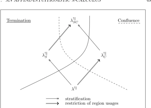
Termination

Our first contributed language is an affine-intuitionistic concurrent λ-calculus in which we can distinguish between values that can be used at most once (i.e. affine) and values that can be duplicated (i.e. intuitionistic). This is made possible by the design of a type system inspired by Linear Logic which takes the duplication power of side effects into account. The difficulty of the contribution is to show the subject reduction (i.e. well-typing is preserved by reduction) of the type system in which the bang modality interacts with region types. The distinction between affine and intuitionistic values allows us to develop a proper discipline of region usages that can be used to ensure the confluence of programs. Moreover, we show that region usages smoothly combine with the discipline of region stratification which ensures the termination of program. The stratifi-cation of regions has been initially proposed by G. Boudol [Bou10] to ensure the termination of higher-order concurrent program in a purely intuitionistic setting.

The above contribution has been presented at the workshop LOLA’10 [ABM10].

Elementary time

Our second contributed language is an elementary concurrent λ-calculus. We provide an elementary affine type system inspired by EAL that ensures the termination of programs in elementary time under a call-by-value strategy, and their progress (i.e. they do not go wrong). In particular, the type system cap-tures the iteration of functions producing side effects over inductive data struc-tures.

The results are supported by the following essential contributions:

• The type system is actually built out of a more primitive depth system which only controls the depth of values. The functional core of the depth system is inspired by the Light Affine λ-calculus of K. Terui [Ter07] and the effectful side relies on a careful analysis of the impact of side effects on the depth of values.

• Programs well-formed in the depth system are shown to terminate in el-ementary time under a call-by-value strategy. The proof is based on an original combinatorial analysis of programs which does not assume ter-mination (i.e. regions stratification is not necessary). Interestingly, in the

(25)

purely functional case, the combinatorial argument applies to every reduc-tion strategy while previous proofs assume a specific reducreduc-tion strategy. The above contribution has been published in the proceedings of TLCA’11 [MA11].

Polynomial time

Our third contributed language is a polynomial concurrent λ-calculus. We pro-vide a light linear type system inspired by LLL that ensures the termination of programs in polynomial time under a call-by-value strategy, and their progress. As in the elementary case, the type system captures the iteration of functions producing side effects, but it is of course less permissive.

Contrary to the elementary case, we found no combinatorial argument to bound polynomially the complexity of the call-by-value evaluation. Thus, we propose a method which follows Terui’s work on the Light Affine λ-calculus [Ter07]:

1. We provide a light linear depth system which controls the depth of values during the reduction of programs. We are able to show that a very spe-cific evaluation strategy terminates in polynomial time by a combinatorial argument which is simply extended from Terui’s work.

2. Since the polynomial evaluation strategy is really different from call-by-value, we try to show that every call-by-value reduction sequence can be transformed into one of the same length that follows the previous evalua-tion strategy, which would entail that call-by-value is polynomial. This latter transformation is non-trivial because it requires to evaluate side effects in a very liberal order. On the other hand, we show that the arbitrary evaluation of side effects may trigger an exponential blowup of the size of the computation. Therefore, our contribution is to identify a proper evaluation strategy for which the transformation succeeds (i.e. returns sequences of the same length) and that preserves the call-by-value semantics of the program. The above contribution has been published in the proceedings of PPDP’12 [Mad12].

Quantitative realizability

The above static criteria (depth systems, type systems) induce complexity bounds which are proved by combinatorial analyzes and syntactic transformations. Our last contribution is to provide an alternative semantic proof of these complexity bounds. More precisely, the framework of quantitative realizability has been pro-posed by Dal Lago and Hofmann [LH11] to give semantic proofs of complexity soundness of various Light Logics. We introduce an extension of quantitative realizability to higher-order imperative programs, focusing on a type system in-spired by LAL. By proving that the type system is sound with respect to the

(26)

1.7. STRUCTURE 25 realizability model, we obtain that every typable program terminates in poly-nomial time under a call-by-value strategy. In particular, we do not need to simulate call-by-value reductions by any other reductions. Moreover, the proof method is parametric in the type system and could easily be adapted to the elementary case.

Our interpretation is based on bi-orthogonality (`a la Krivine [Kri09]), following A. Brunel’s extension of quantitative realizability to a classical setting [Bru12]. Realizability in the presence of imperative side effects is usually difficult as it raises circularity issues; here, our semantic interpretation is indexed by depth levels which allows to define an inductive interpretation of types. This draws some interesting connections with other realizability models based on step-indexing [AM01] and Nakano’s modality [Nak00].

The important drawback of the method is that, at the moment, it does not scale to multi-threaded programs.

This last contribution is joint work with Alo¨ıs Brunel and is to published in the proceedings of APLAS’12 [BM12].

1.7 Structure

This document is structured into three parts: I - Termination and Confluence

The first part is preliminary to the analysis of the complexity of programs. In Chapter 2, we review a concurrent λ-calculus and the discipline of region stratification. In Chapter 3, we introduce an affine-intuitionistic concurrent λ-calculus and show how termination and confluence can be ensured by region stratification and region usages, respectively.

II - Combinatorial and Syntactic Analyzes

The second part introduces static criteria to control the complexity of pro-grams and the complexity bounds are proved by combinatorial syntactical analyzes. The first Chapter4 and Chapter5 deal with elementary time and the last Chapter 6 and Chapter 7 deal with polynomial time. Each time we start by reviewing the purely functional case before moving to concurrency.

III - Quantitative Realizability (joint work with Alo¨ıs Brunel)

The unique Chapter 8introduces quantitative realizability for an imper-ative λ-calculus. As a case study, we focus on termination in polynomial time.

(27)

(28)

Part I

Termination and

Confluence

(29)

(30)

Chapter 2

A concurrent λ-calculus

We present in this chapter an extension of the λ-calculus to concurrency which is based on R. Amadio’s formalization [Ama09]. In this λ-calculus, that we call λk, the state of a program is abstracted by a constant number of regions and side effects are produced by read and write operations on these regions. In fact, a region is an abstraction of a set of dynamically allocated values. We will see that working at the abstract level of regions allows to simulate various interaction mechanisms like imperative references and communication channels. In this chapter, we also present a technique to establish the termination of higher-order concurrent programs. Indeed, the property of termination may be seen as preliminary to the property of termination in bounded time, the latter being central in this thesis. The Curry-Howard correspondence estab-lishes a well known connection between the termination of purely functional programs and types. However, side effects are not taken into account by the usual type systems and they may make programs diverge. Type and effect sys-tems have been introduced by J. Lucassen and D. Gifford [LG88] to approximate the way programs act on regions. Later, they have been used by M. Tofte and J-P. Talpin [TT97] to determine statically the management of memory. Recently, G. Boudol [Bou10] introduced a discipline of region stratification by means of a type and effect system, to show the termination of higher-order concurrent programs. This chapter presents the discipline of region stratification in a way that has been clarified and generalized by R. Amadio [Ama09].

Outline This chapter is organized as follows. In Section 2.1 we present the syntax and the reduction of the concurrent λ-calculus λk. The reduction rules are defined such that λk simulates a concurrent λ-calculus with references or channels. In Section2.2we present the type and effect system. Here, the effect of a program is an over approximation of the set of regions it may read or write. This type and effect system allows some form of circularity: a region r can

(31)

contain a value which has an effect on r itself, and this may lead to a diverging computation. In Section2.3we introduce the discipline of region stratification to prevent this kind of circularity. The intuitive idea is that a region may only produce side effects on regions which are smaller according to a well-founded order. Then we review the proof by reducibility candidates which proves that well-typed stratified programs terminate. Finally, in Section2.4we present two additional concurrent λ-calculi: one with dynamic allocation of references and one with dynamic allocation of channels, that are respectively called λkRef and λkChan. We show that the abstract language with regions, namely λk, simulates both λkRef and λkChan. Since we can lift the stratification of regions to the lan-guages with dynamic values, we are able to show the termination of concurrent programs with references and channels.

A summary of the presented calculi is illustrated in Figure2.1. For any calculi

λkChan_S _- λk_S _% λkRef_S

Termination

λkChan _- λk _% λkRef stratification

Figure 2.1: Stratification entails termination in every calculi

X, Y , the relation X % Y stands for X simulates Y , and XS stands for the

stratified version of X. We see that in any case, stratified or not, the calcu-lus with region λk simulates both the one with references λkRef and the one with channels λkChan. Stratification can be lifted to every calculus and entails termination.

2.1 Syntax and reduction

The concurrent λ-calculus λkis a call-by-value λ-calculus equipped with regions and parallel composition. We recall that a region is an abstraction of a set of dynamically generated values like references and channels. We regard λk _{as an}

abstract, highly non-deterministic language which, as we will see in Section2.4, simulates more concrete languages like λkRef and λkChan.

(32)

2.1. SYNTAX AND REDUCTION 31

2.1.1 Syntax

of variables x, y, . . . and we also have a set of regions r, r0, . . . Values contain integers, variables, regions, the unit value ? and λ-abstractions. Terms are made of values, applications, an operator get(r) to read a value from region, an operator set(r, V ) to assign a value to a region and the parallel composition (M k N ) to evaluate M and N concurrently. A store S is the composition of several assignments r ⇐ V in parallel and a program P is the combination of several terms and stores in parallel. Note that stores are global, i.e. they always occur in empty contexts.

The set of free variables of M is denoted by FV(M ). The capture-avoiding substitution is written M [V /x] and denotes the term M in which each free occurrence of x has been substituted by V . As usual the sequential composition M ; N can be encoded by (λx.N )M where x /∈ FV(N ).

2.1.2 Reduction

The call-by-value reduction of λk is given in Figure2.3 which we comment in the following paragraphs.

Programs are considered up to a structural equivalence ≡ which is the least equivalence relation that contains the equations for α-renaming, commutativity and associativity of parallel composition.

We distinguish two kinds of contexts. An evaluation context E specifies a left-to-right call-by-value evaluation strategy. A static evaluation context C acts as an arbitrary scheduler which chooses a random thread to evaluate.

The structural equivalence ≡ is only preserved by static evaluation contexts. For example we have

(33)

-structural rules-P k rules-P0 _≡ _P0 _{k P} (P k P0_{) k P}00 _≡ _{P k (P}0 _{k P}00₎ -evaluation contexts-E ::= [·] | EM | V E C ::= [·] | (C k P ) | (P k C) -reduction rules-(βv) C[E[(λx.M )V ]] −→ C[E[M [V /x]]]

(get) C[E[get(r)]] k r ⇐ V −→ C[E[V ]] k r ⇐ V

(set) C[E[set(r, V )]] −→ C[E[?]] k r ⇐ V

Figure 2.3: Call-by-value reduction of λk

where the program (P1k P2) occurs in the static context C = ([·] k P3) but

(λx.M k N )V 6≡ (λx.N k M )V

where (M k N ) occurs under a λ-abstraction in the context E = [·]V .

The reduction rules apply modulo structural equivalence and each rule is iden-tified by its name: (βv) is the usual β-reduction restrained to values; (get) is for

reading some value from a region and (set) is for adding a value to a region. We remark that the reduction rule (set) generates an assignment which is new and out of the evaluation contexts; this implies two things:

1. Store assignments are global and shared by every threads.

2. Store assignments are cumulative, that is several values can be assigned to a region. We will see that this allows a single region to abstract an unlimited number of memory locations. In turn, reading a region consists in getting non-deterministically one of the assigned values.

The reader may have noticed that the program set(r, M ) is not generated by the syntax if M is not a value. This choice simplifies the shape of evaluation contexts since we do not need to consider the context set(r, E). On the other hand, this does not cause any loss of expressivity since we consider that set(r, M ) is syntactic sugar for (λx.set(r, x))M .

Example 2.1.1. Here is a programming example. Assume we dispose of inte-gers z for z ∈ Z and their basic operators. Consider the following function F that takes three arguments g, h and x:

F = λg.λh.λx.set(r, gx) k set(r, hx) k get(r) + get(r)

It generates three concurrent threads which respectively do the following: writ-ing the result of the application gx into the region r, writwrit-ing the result of the

(34)

2.2. TYPE AND EFFECT SYSTEM 33 application hx into the region r and reading the region r twice to sum the values. Now consider the following arguments:

G = λx.x + 1 H = λx.2

One possible reduction when we apply F to G, H and z is:

((F G)H)z −→+ _{set(r, Gz) k set(r, Hz) k get(r) + get(r)}

−→+ _{? k ? k get(r) + get(r) k r ⇐ z + 1 k r ⇐ 2}

−→ ? k ? k z + 1 + get(r) k r ⇐ z + 1 k r ⇐ 2 −→ ? k ? k z + 1 + 2 k r ⇐ z + 1 k r ⇐ 2 −→ ? k ? k z + 3 k r ⇐ z + 1 k r ⇐ 2

Other possible reductions lead to structurally equivalent programs, except that we may find the value 2z + 2 or 4 instead of z + 3, depending on which value is read from the region r.

2.2 Type and effect system

As we explained in the introduction of this chapter, usual types systems cannot take side effects into account and thus cannot serve to establish the termination of concurrent programs. In this section, we present a type and effect system to statically determine the regions on which side effects are produced. Our formalism is the one proposed by R. Amadio [Ama09]. We will see in the next section how this type and effect system can be used to entail the termination of programs.

2.2.1 Types and contexts

The starting point is to consider effects, denoted with e, e0, . . . as finite sets of regions. Then, the functional type is annotated with an effect e such that we write

A−→ Be

for the type of a function that, when given a value of type A, produces side effects on the regions in e and returns a program of type B.

We define the syntax of types and contexts in Figure 2.4. We distinguish two kinds of types:

1. General types are denoted with α, α0_{, . . . and contain a special behavior}

type B which is given to stores or concurrent threads which are not sup-posed to return a value but just to produce side effects.

(35)

-effects e, e0, . . .

-types α ::= B | A

-value types A ::= Unit | A−→ α | Rege rA

-variable contexts Γ ::= x1: A1, . . . , xn: An

-region contexts R ::= r1: A1, . . . , rn : An

Figure 2.4: Syntax of types, effects and contexts

2. Value types are denoted with A, B, . . . and are types of entities that may return a value. The only ground type is the unit type Unit. The functional type A−→ α ensures that functions are only given values as argument bute may return a program which evaluates into a value or several concurrent threads. The type Reg_rA is the type of the region r containing values of type A. Hereby types may depend on regions.

We distinguish also two kinds of contexts.

1. Variable contexts are made of distinct variables that are associated to value types, thus we will not be able to build a program of type B−→ α.e We write dom(Γ) for the set {x1, . . . , xn}.

2. Region contexts are made of distinct regions that are associated to value types. The typing system will guarantee that whenever we use a type Reg_rA the region context contains a hypothesis r : A. Thus we will not be able to store non-values in regions. We write dom(R) for the set {r1, . . . , rn}.

The region type Reg_rA is carrying an explicit name of region. As we will see in Section2.4, this dependency between types and regions allows to simulate a calculus with dynamic locations by a calculus with regions. However, we have to be careful in defining the following notions:

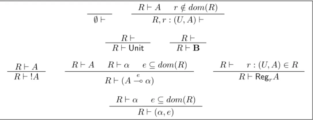
• A type is compatible with a region context (judgment R ↓ α). • A region context is well-formed (judgment R `).

• A type is well-formed in a region context (judgment R ` α), a variable context is well-formed in a region context (R ` Γ), and a type and effect is well-formed in a region context (judgment R ` (α, e)).

The rules of these judgments are given in Figure2.5. A more informal way to express these conditions is to say that a judgment r1 : A1, . . . , rn : An ` α is

well formed provided that:

1. All the region names occurring in the types A1, . . . , An, α belong to the

set {r1, . . . , rn},

2. All types of the shape RegriB with i ∈ {1, . . . , n} and occurring in the types A1, . . . , An, α are such that B = Ai.

(36)

2.2. TYPE AND EFFECT SYSTEM 35 R ↓ Int R ↓ Unit R ↓ B R ↓ A R ↓ α e ⊆ dom(R) R ↓ A−→ αe r : A ∈ R R ↓ Reg_rA ∀r : A ∈ R R ↓ A R ` R ` R ↓ α R ` α ∀x : A ∈ Γ R ` A R ` Γ R ` α e ⊆ dom(R) R ` (α, e)

Figure 2.5: Formation of types and contexts

Example 2.2.1. The judgment r : Unit −−→ Unit ` can be derived while the{r} judgments r1 : Regr2Unit

{r2}

−−−→ Unit, r2 : Unit {r1}

−−−→ Unit ` and r : RegrA `

cannot.

2.2.2 Rules

A typing judgment has the shape

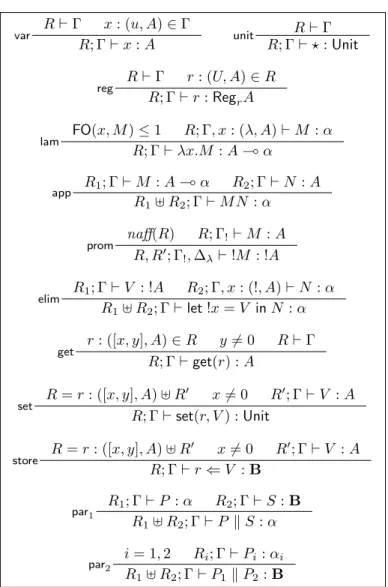
R; Γ ` P : (α, e)

It gives the type α to the program P and the effect e is an upper bound on the set of regions that P may read or write. Effects are simply built by exploiting the region names occurring in the syntax; in particular, we can be sure that values and stores produce an empty effect while the terms get(r) and set(r, V ) produce an effect {r}. The rules of the type and effect system are spelled out in Figure2.6.

Remark 2.2.2. Here are some remarks on the rules.

• Contexts are the same in every rule and each axiom (namely var, unit and reg) has a premise R ` Γ which ensures that, in all branches of the typing derivations, every type is well-formed with respect to the region context. • Effects are initialized by the rules get and set by referring to the explicit

region name of the read/write operator.

• We notice in the rule lam how the effect of a term ends up on the functional arrow in order to build a λ-abstraction with empty effect. Finally, binary rules handle effects in an additive way by set union.

• We distinguish two rules for parallel composition. par1 indicates that

(37)

var R ` Γ x : A ∈ Γ R; Γ ` x : (A, ∅) unit R ` Γ R; Γ ` ? : (Unit, ∅) reg R ` Γ r : A ∈ R R; Γ ` r : (Reg_rA, ∅) lam R; Γ, x : A ` M : (α, e) R : Γ ` λx.M : (A−→ α, ∅)e app R; Γ ` M : (A e1 −→ α, e2) R; Γ ` N : (A, e3) R; Γ ` M N : (α, e1∪ e2∪ e3) get R; Γ ` r : (RegrA, ∅) R; Γ ` get(r) : (A, {r})

set R; Γ ` r : (RegrA, ∅) R; Γ ` V : (A, ∅)

R; Γ ` set(r, V ) : (Unit, {r})

store R; Γ ` r : (RegrA, ∅) R; Γ ` V : (A, ∅)

R; Γ ` r ⇐ V : (B, ∅) par1 R; Γ ` P : (α, e) R; Γ ` S : (B, ∅) R; Γ ` P k S : (α, e) par2 i = 1, 2 R; Γ ` Pi: (αi, e1) Pi not a store R; Γ ` P1k P2: (B, e1∪ e2)

(38)

2.2. TYPE AND EFFECT SYSTEM 37 we might be interested in its result. par₂ indicates that two concurrent threads cannot reduce to a single result. (note that we have omitted the symmetric rules to support commutativity of parallel composition). We notice that the following rules can be derived for syntactic sugar set(r, M ):

setM

R; Γ ` r : (Reg_rA, ∅) R; Γ ` M : (A, e) R; Γ ` set(r, M ) : (Unit, e ∪ {r}) Example 2.2.3. The program F of Example2.1.1written

F = λg.λh.λx.set(r, gx) k set(r, hx) k get(r) + get(r) can be given the following typing judgment:

R; − ` F : ((A−→ Int)∅ −→ (A∅ −→ Int)∅ −→ A∅ −−→ B, ∅){r}

where r : Int ∈ R. Also, the programs G = λx.x + 1 and H = λx.2 can be given the type and effect (Int−→ Int, ∅) in order to derive the following judgment:∅

R; − ` ((F G)H)z : (B, {r})

Subtyping

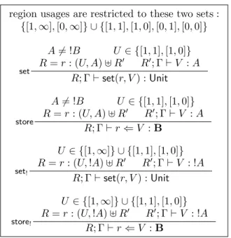
In some cases, the presence of effects may be unnecessarily restrictive. For example, suppose that we first want to write into a region r a value V1 of type

Unit −→ Unit that may not produce any side effect; then we want to add to r∅ another value V2 of type Unit

e

−→ Unit where e ) ∅. Considering that a region context associates a unique type to the region r, one of the assignments is not typable.

In order to allow for some flexibility, it is convenient to introduce a subtyping relation on types (judgment R ` α ≤ α0) and on types and effects (judgment R ` (α, e) ≤ (α0, e0)) as specified in Figure2.7. Intuitively, the new subtyping

R ` α ≤ α e ⊆ e0⊆ dom(R) R ` A0≤ A R ` α ≤ α0 R ` (A−→ α) ≤ (Ae 0 e₋_{→ α}0 0₎ e ⊆ e0⊆ dom(R) R ` α ≤ α0 R ` (α, e) ≤ (α0_{, e}0₎ sub R; Γ ` M : (α, e) R ` (α, e) ≤ (α0, e0) R; Γ ` M : (α0_{, e}0₎

Figure 2.7: Subtyping induced by effect containment

(39)

or the effect of a program becomes an upper bound of the set of regions that may be read/written.

Back to our initial problem, let us define a region context R such that r : Unit−→e Unit ∈ R where e ) ∅. By using the subtyping rule, we can give the type and effect (Unit −→ Unit, ∅) to the effect free value Ve 1 = λx.x with the following

derivation:

R; x : Unit ` x : (Unit, ∅)

sub

R; x : Unit ` x : (Unit, e) R; − ` λx.x : (Unit−→ Unit, ∅)e

Now take the value V2 of type and effect (Unit e

−

→ Unit). Finally, the program that writes V1 and V2to r can be given the judgment

R; − ` set(r, V1); set(r, V2) : (Unit, {r})

We notice that the transitivity rule for subtyping R ` α ≤ α0 R ` α0 ≤ α00

R ` α ≤ α00

can be derived via a simple induction on the height of the proofs. Moreover, the introduction of the subtyping rules has a limited impact on the structure of the typing proofs. Indeed, if R ` A ≤ B then we know that A and B may just differ in the effects annotating the functional types. In particular, when looking at the proof of the typing judgment of a value such as R; Γ ` λx.M : (A, e), we can always argue that A has the shape A1

e1

−→ A2and, in case the effect e is not

empty, that there is a shorter proof of the judgment R; Γ ` λx.M : (B1 e2 −→ B2, ∅)

where R ` A1≤ B1, R ` B2≤ A2, and e2⊆ e1.

2.2.3 Properties

The usual properties of type systems can be adapted to the type and effect system.

First, it is possible to weaken variable and region contexts, provided that they are well-formed.

Lemma 2.2.4 (Weakening). If R; Γ ` P : (α, e) and R, R0 ` Γ, Γ0 _then

R, R0; Γ, Γ0` P : (α, e).

Typing is also preserved when we substitute a variable for an effect free value of the same type.

Lemma 2.2.5 (Substitution). If R; Γ, x : A ` P : (α, e) and R; Γ ` V : (A, ∅) then R; Γ ` P [V /x] : (α, e).

(40)

2.2. TYPE AND EFFECT SYSTEM 39 The above lemmas can be shown by induction on the typing judgments and they are needed to prove subject reduction. Let us write S_|f as the store S restricted to the regions in f , for any set of regions f .

Proposition 2.2.6 (Subject reduction). If R1, R2; Γ ` P k S : (α, e) and

P k S −→ P0k S0 _{and R} 1` (α, e) then: 1. R1, R2; Γ ` P0 k S0 : (α, e), 2. P k S|dom(R1)−→ P 0_{k S}0 |dom(R1) and S 0 |dom(R2)= S|dom(R2).

The first statement simply says that the type and effect is preserved by reduc-tion. The second statement guarantees that the program can only read/write regions included in the region context needed to the well-formation of the type and effect. More generally, this shows that that the effect of a program is an upper bound of the set of regions on which side effects are produced. The proof of this statement can be shown by checking that if a program C[E[M ]] has an effect e and M = get(r) or M = set(r, V ), then r ∈ e.

Finally, a progress property states that if a program cannot reduce, then every thread is either a value or a term of the shape E[get(r)] where the region r is empty.

Proposition 2.2.7 (Progress). Suppose P is a typable program which cannot reduce. Then P is structurally equivalent to a program

M1k · · · k Mmk S m ≥ 0

where Mi is either a value or can be uniquely decomposed as a term E[get(r)]

such that no assignment to r exists in the store S.

The proof is standard and mainly consists in showing that a closed value of type A−→ B must have the shape λx.M , so that a well-typed closed program V N ise guarantee to reduce.

2.2.4 Recursion

The current type and effect system allows to write in a region r a function λx.M where M produces an effect on r itself, for instance λx.get(r)x. This kind of circularity may lead to diverging computations like the following one:

set(r, λx.get(r)x); get(r)? −→∗ _{get(r)? k r ⇐ λx.get(r)x}

−→ (λx.get(r)x)? k r ⇐ λx.get(r)x −→ get(r)? k r ⇐ λx.get(r)x −→ . . .

This circularity can be used to define an imperative fixpoint combinator, also well-known as Landin’s trick. More precisely, we define a combinator

(41)

that relates to a region r and binds f in M . Then the following reduction rule can be derived:

(µr) (µrf.λx.M )V −→ M [λy.get(r)y/f, V /x] k r ⇐ λx.M [λy.get(r)y/f ]

As an example, this combinator can be used to define a counter that keeps being incremented forever and each time writes its value to a region r0. Take

λx.M = λx.set(r0, x); f (x + 1) Then we observe (µrf.λx.M )0 −→∗ _{M [λy.get(r)y/f, 1/x] k r ⇐ λx.M [λy.get(r)y/f ] k r}0_{⇐ 0} −→∗ _{M [λy.get(r)y/f, 2/x] k r ⇐ λx.M [λy.get(r)y/f ] k r}0_{⇐ 0 k r}0 _{⇐ 1} −→∗ _{M [λy.get(r)y/f, 3/x] k r ⇐ λx.M [λy.get(r)y/f ] k r}0_{⇐ 0 k r}0 _{⇐ 1 k r}0 _{⇐ 2} −→∗ . . .

Although the type and effect system takes side effects into account, it does not prevent circularities and the following rule can be derived:

fix R, r : A e∪{r} −−−−→ α; Γ, f : A−−−−→ α ` λx.M : (Ae∪{r} −−−−→ α, ∅)e∪{r} R; Γ ` µrf.λx.M : (A e∪{r} −−−−→ α, ∅)

2.3 Termination

G. Boudol introduced [Bou10] the discipline of stratified regions in order to recover the termination of concurrent programs. Intuitively, the idea is to fix a well-founded order on regions and make sure that the values stored in a given region may only produce side effects on smaller regions. Back to the type and effect system, stratification means that a value of type Unit−−→ Unit can only{r} be stored in regions which are larger than r. This discipline can be easily ensured by redefining the rules of Figure 2.5governing the formation of types and contexts .

We give new definitions of the judgments R `, R ` α and R ` (α, e) in Fig-ure2.8. Regions are thus ordered from left to right, that is if the judgment

r1: A1, r2: A2, . . . , ri: Ai, . . . , rn: An`

can be derived, effects occurring in Ai may only contain regions rjwhere j < i.

We denote by ‘`S’ provability in the system where the rules for the formation

of unstratified region contexts (Figure 2.5) are replaced by the rules for the formation of stratified region contexts (Figure 2.8). We call λk_S the stratified concurrent λ-calculus. The fixpoint rule fix given in the previous section cannot be derived in `S since the region context is not stratified (the type of region r

(42)

2.3. TERMINATION 41 ∅ ` R ` A r /∈ dom(R) R, r : A ` R ` R ` Unit R ` R ` Int R ` R ` B R ` A R ` α e ⊆ dom(R) R ` (A−→ α)e R ` r : A ∈ R R ` Reg_rA R ` α e ⊆ dom(R) R ` (α, e)

Figure 2.8: Stratified formation of types and contexts

Theorem 2.3.1 (Termination). If R; Γ `S P : (α, e) then P terminates.

The proof is based on an extension of the reducibility candidates method to programs with stores and was originally presented in G. Boudol’s paper [Bou10] and later simplified by R. Amadio [Ama09]. The latter version of the proof can be summarized in the following items.

• The starting idea is to define the interpretation R ` of a stratified region context R as a set of stores and to define the interpretation R ` (α, e) of a type and effect (α, e) as a set of terms that terminate with re-spect to stores of R `. The interpretations are thus mutually defined but well-founded because stratification allows for an inductive definition of the stored values. For instance, the interpretation r1: A1, r2: A2` (α, e)

refers to r1: A1, r2: A2` which is a set of stores where all the values of r2

can only have an effect on r1 and thus belong to r1: A1` (A2, e), which

in turn refers to the ‘smaller’ interpretation r1: A1`,. . .

• A key point of the proof is that region contexts are interpreted as ‘sat-urated’ stores which already contains all the values that can be possibly written. This gives a simple argument to extend the proof to concurrent programs. Indeed, we know that each thread taken separately terminates with respect to a saturated store. If the parallel composition of a set of threads diverges, then one of the threads must diverge. But since the saturated store cannot be updated by the set of threads, this contradicts the hypothesis that each single thread taken apart terminates.

In Chapter8, we give another realizability interpretation that takes quantitative information into account so that the length of reductions of an imperative λ-calculus can be bounded.

(43)

2.4 Dynamic locations

To conclude this chapter, we introduce a type and effect system for two con-current λ-calculi with dynamic memory locations instead of regions: one with references that we call λkRef, and one with channels that we call λkChan. Since λkRef and λkChan still relate to regions at the level of types, we are able to lift the stratification discipline to these calculi. Moreover, λk simulates λkRef and λkChan _{by exact correspondence of reduction steps, therefore we can prove the}

termination of λkRef and λkChan.

First, let us present the relation between the systems with dynamic locations and the system with abstract regions informally. In λk, read and write operators refer to region names. On the other hand, the languages λkChan and λkRef introduce terms of the form νx.M to generate a new memory location x whose scope is M . We can thus write a program

νx.(λy.set(y, V ); get(y))x

that generates a fresh location x and gives it as argument to a function that writes and reads at this location. In ML style, this would correspond to the program

let x = ref V in !x

There is a simple typed translation from λkChan and λkRef to λk. For this, a memory location must be a variable that relates to an abstract region r by having the type Reg_rA for some type A. Then the translation consists in replacing each (free or bound) variable that relates to a region r by the name r. We will see that the program with regions obtained by translation simulates the original because each reduction step in λkChanand λkRefis mapped to exactly one reduction step of λk. Therefore we can apply the termination theorem to λkChan and λkRef. The formalization of λkChan and λkRef is summarized in Figure2.9. They have the same syntax and typing rules, they only differ in their reduction rules. Concretely:

• The syntax of the languages does not contain region names, instead read and write operators and stores relate to memory locations (that is vari-ables). We also find a ν binder with two associated structural rules (νE)

and (νC) for scope extrusion.

• Each language has its own set of reduction rules (in addition to (βv)).

Specifically, when we read a reference the value is copied from the store and when we write a reference the value overwrites the previous one (we assume that the ν binder generates a location with a dummy value that is overwritten at the first write). When we write a channel we add the value to the store and when we read a channel we consume one of the value in the channel. Thus channels are asynchronous, unbounded and unordered.

(44)

2.4. DYNAMIC LOCATIONS 43

-extended

syntax-M ::= . . . | get(x) | set(x, V ) | νx.M S ::= x ⇐ V | (S k S)

E ::= . . . | νx.E

-new structural

rules-(νC) C[νx.M ] ≡ νx.C[M ] if x /∈ FV(C)

(νE) E[νx.M ] ≡ νx.E[M ] if x /∈ FV(E)

-reductions rules of λkRef

-(get ref) C[E[get(x)]] k x ⇐ V −→ C[E[V ]] k x ⇐ V

(set ref) C[E[set(x, V )]] k x ⇐ V0 _−→ _{C[E[?]] k x ⇐ V}

-reductions rules of λkChan

-(get chan) C[E[get(x)]] k x ⇐ V −→ C[E[V ]]

(set chan) C[E[set(x, V )]] −→ C[E[?]] k x ⇐ V

-additional and replacing typing

rules-new R; Γ, x : RegrA ` M : (B, e)

R; Γ ` νx.M : (B, e) get

R; Γ ` x : (Reg_rA, ∅) R; Γ ` get(x) : (A, {r})

set R; Γ ` x : (RegrA, ∅) R; Γ ` V : (A, ∅)

R; Γ `δ set(x, V ) : (Unit, {r})

store R; Γ ` x : (RegrA, ∅) R; Γ ` V : (A, ∅)

R; Γ ` x ⇐ V : (B, ∅)

Figure 2.9: Overview of λkChan and λkRef

• The typing rule reg is no longer necessary but we introduce a rule called new that allows to bind variables of region type. The rules get, set and store replace the previous ones and the effect of programs can still be inferred by referring to the region names occurring in the types of memory locations.

Clearly, subject reduction (Proposition 2.2.6) and progress (Proposition2.2.7) can be lifted to λkChanand λkRef.

Concerning termination, the proof goes by a translation phase from λkChan _or

(45)

program-ming example of λkRef. Consider the following reduction: νx.νy.(λz.set(z, n) k set(y, get(z)))x −→ νx.νy.set(x, n) k set(y, get(x)) −→ νx.νy.? k set(y, get(x)) k x ⇐ n −→ νx.νy.? k set(y, n) k x ⇐ n −→ νx.νy.? k ? k x ⇐ n k y ⇐ n

The location x is passed to a function which generates two threads. The first thread writes an integer n in reference x, the second thread read n from reference x and propagates it into reference y. The program may be given the following type and effect derivation by taking that references x and y relate to a single region r:

.. .

r : Int; x : Reg_rInt, y : Reg_rInt ` (λz.set(z, n) k set(y, get(z)))x : (B, {r}) r : Int; − ` νx.νy.(λz.set(z, n) k set(y, get(z)))x : (B, {r})

The translation consists in (1) erasing all ν binders and (2) replacing each variable of region type with the corresponding region name. This gives us the following program whose reductions steps are in one-to-one correspondence with the original reductions:

(λz.set(r, n) k set(r, get(r)))r −→ set(r, n) k set(r, get(r)) −→ ? k set(r, get(r)) k r ⇐ n −→ ? k set(r, n) k r ⇐ n −→ ? k ? k r ⇐ n k r ⇐ n

We observe that the region r ‘accumulates’ two values n because r relates to two references x and y. In general, the λk program may produce additional assignments since stored values are never erased, but at least one reduction sequence will simulate the original one. The translated program can be given the following type and effect

r : Int; − ` (λz.set(r, n) k set(r, get(r)))r : (B, {r})

which is the same as the original program except that the free memory locations x and y do not occur anymore in the variable contexts of the derivation. Since the stratification of regions is preserved by translation we can conclude that the stratified systems λkRef_S and λkChan_S terminate. Indeed, if there is an infinite reduction in λkRef_S or λkChan_S , there must be an infinite reduction in λk and this contradicts Theorem2.3.1.

It should be noted that using a single region r to abstract every locations is a rather drastic solution. In our example, we could have alternatively associated a distinct region to each channel x and y. In the context of region-based memory

(46)

2.4. DYNAMIC LOCATIONS 45 management [TT97], the problem of region inference which consists in finding an assignment from locations to regions in the most optimal way with respect to the performance of the language is a crucial question which is beyond the scope of this thesis. The reader may consult a report on the MLKit compiler [TBE+₀₆_]

that implements a based garbage collector; a retrospective on region-based memory management is also available [TBEH04].

(47)

Complexité Implicite de Lambda-Calculs Concurrents

HAL Id: tel-00794977

https://tel.archives-ouvertes.fr/tel-00794977

Submitted on 26 Feb 2013

HAL is a multi-disciplinary open access

archive for the deposit and dissemination of

sci-entific research documents, whether they are

pub-lished or not. The documents may come from

teaching and research institutions in France or

abroad, or from public or private research centers.

L’archive ouverte pluridisciplinaire HAL, est

destinée au dépôt et à la diffusion de documents

scientifiques de niveau recherche, publiés ou non,

émanant des établissements d’enseignement et de

recherche français ou étrangers, des laboratoires

publics ou privés.

Antoine Madet

To cite this version:

Antoine Madet. Complexité Implicite de Lambda-Calculs Concurrents. Programming Languages

[cs.PL]. Université Paris-Diderot - Paris VII, 2012. English. �tel-00794977�

Universit´

e Paris Diderot (Paris 7)

Laboratoire Preuves, Programmes, Syst`

emes

´

Ecole Doctorale Sciences Math´

ematiques de Paris Centre

Th`

ese de doctorat

Sp´

ecialit´

e informatique

Complexit´

e Implicite

de

Lambda-Calculs

Concurrents

Antoine Madet

Soutenue le 6 d´

ecembre 2012

devant le jury compos´

e de:

M. Roberto Amadio

Directeur

M. Patrick Baillot

Directeur

M. Ugo Dal Lago

Rapporteur

M. Jean-Yves Marion

Rapporteur

M. Virgile Mogbil

Examinateur

Remerciements

Implicit Complexity

in

Contents

I

Termination and Confluence

27

II

Combinatorial and Syntactic Analyzes

75

III

Quantitative Realizability

151

Chapter 1

Introduction

1.1

Higher-order concurrent programs

1.2

Proofs as programs

1.3

Implicit Computational Complexity

1.4

Light Logics

1.5

The challenge

1.6

Contributions

1.7