HAL Id: hal-00002323
https://hal.archives-ouvertes.fr/hal-00002323
Submitted on 27 Jul 2004
HAL is a multi-disciplinary open access
archive for the deposit and dissemination of
sci-entific research documents, whether they are
pub-lished or not. The documents may come from
teaching and research institutions in France or
abroad, or from public or private research centers.
L’archive ouverte pluridisciplinaire HAL, est
destinée au dépôt et à la diffusion de documents
scientifiques de niveau recherche, publiés ou non,
émanant des établissements d’enseignement et de
recherche français ou étrangers, des laboratoires
publics ou privés.
Two-fluid model for VLBI jets. I. Homogeneous and
stationary synchrotron emission simulations
Vincent Despringre, Didier Fraix-Burnet
To cite this version:
Vincent Despringre, Didier Fraix-Burnet. Two-fluid model for VLBI jets. I. Homogeneous and
sta-tionary synchrotron emission simulations. Astronomy and Astrophysics - A&A, EDP Sciences, 1997,
320, pp.26-32. �hal-00002323�
ccsd-00002323, version 1 - 27 Jul 2004
(will be inserted by hand later) Your thesaurus codes are:
03 (02.18.5; 03.13.4 11.01.2 11.10.1 13.18.1)
ASTRONOMY AND ASTROPHYSICS
27.7.2004
Two-fluid model for VLBI jets
I. Homogeneous and stationary synchrotron emission simulations.
V. Despringre1 and D. Fraix-Burnet21
Laboratoire d’Astrophysique de Toulouse UMR 5572, Observatoire Midi-Pyr´en´ees, 14 Avenue Edouard Belin, F-31400 Toulouse, France, [email protected]
2
Laboratoire d’Astrophysique UMR 5571, Observatoire de Grenoble, BP 53, F-38041 Grenoble C´edex 9, France, [email protected]
Received June 13, 1996; accepted September 18, 1996
Abstract. In this series of papers, we develop a two-fluid model for VLBI jets. The idea is that the jet itself is non-or mildly-relativistic (electrons and protons), while the radiating blobs are relativistic electron-positron ‘clouds’ moving on helical paths wrapped around the jet. In this work, the emphasis is on the physical description of the clouds, and not on the structure or origin of the trajec-tory. In the simple case where the magnetic field is uniform and homogeneous accross the cloud, and the properties of the cloud are constant, the present paper shows synthetic maps of VLBI jets in different configurations, as well as the variation of different observational parameters along the trajectory.
Key words: galaxies : jet – galaxies : actives – radiation mechanisms : non-thermal – radio continuum : galaxies – methods : numerical
1. Introduction
Extragalactic jets at the parsec scale are present in nu-merous Active Galactic Nuclei (AGN; see a review by Zensus 1995). Impressive progress has been made by the Very Large Baseline Interferometry (VLBI), and details still closer to the central engine are expected with the ad-vent of millimeter VLBI. Already, a lot of information can be gained from the structure of these jets with typically 1 parsec resolution. It has been possible to detect motions within a few years in about 100 sources (Vermeulen 1995), a lot of them being superluminal with apparent speeds up to 10c. The motions detected are those of blobs moving on curved trajectories. Generally speaking, these paths are wiggling, reminiscent of more or less helical lines seen in projection, and apparently different from one blob to the
other, and the blob velocities vary along the trajectory (Zensus 1995; Qian et al. 1996).
Not much information is available on the nature of the blobs themselves. They are very generally believed to be shock fronts, because i) shock waves are expected in these jets and ii) they are an excellent means of accelerating particles through the first-order Fermi acceleration process as has been worked out in the kpc scale jets. Recently, in a series of papers, G´omez et al. (1993, 1994a, 1994b) performed numerical simulations of a VLBI jet where the blobs are shock fronts traveling along a helical relativistic jet. Nevertheless, the reality of these shock fronts is far from established.
The hypothesis of a relativistic jet is also debatable. Firstly, due to the Compton drag close to the black hole, it is very difficult to extract a jet with Lorentz factors higher than 2 or 3 (Phinney 1987, Henri & Pelletier 1991). Secondly, at the kpc scale, jets are probably non- or only mildly-relativistic (e.g. Parma et al. 1987, Fraix-Burnet 1992). Some authors conclude that the jets should de-celerate (Bowman et al. 1996) from super- to subluminal speeds, but obviously, the lost energy should be observed in a manner or in another.
An interesting alternative to relativistic shocked jets is the two-fluid concept, in which the bulk of the jet (elec-trons and protons ejected from the accretion disk in the form of a collimated wind) is non- or mildly-relativistic at all scales, and synchrotron radiation is produced by a beam of relativistic electrons/positrons. This idea has been worked out theoretically by Sol, Pelletier and Ass´eo (1989) and applied to kpc jets (Pelletier & Roland 1986, 1988; Fraix-Burnet & Pelletier 1991; Fraix-Burnet 1992) for the particle acceleration problem. At small scales, ob-served relativistic phenomena can be produced by the rela-tivistic electrons/positrons, and Pelletier & Roland (1989) found a very interesting application for cosmology using superluminal radio sources.
2 V. Despringre et al.: Two-fluid model for VLBI jets
In this series of papers, we propose to apply this two-fluid concept to VLBI jets. The idea is based on the cor-relation between outbursts of AGNs and the subsequent appearance of VLBI blobs. If these bursts are explained by bursts of high-energy particles (as in Marcowith et al. 1996), then it is probable that these particles prop-agate on a few parsecs away. A relativistic beam propa-gating within the jet plasma has been shown (Sol et al. 1989; Achatz, Lesch & Schlickeiser 1990; Pelletier & Sol 1992; Achatz & Schlickeiser 1992) to be stable relatively to the excitation of Langmuir, Alfv´en and whistler waves, on scales up to several hundreds of parsecs. Hanasz & Sol (1996) recently showed that large scale fluid (Kelvin-Helmoltz) stability is also possible. Hence, we suggest that the blobs seen in VLBI jets are these ‘clouds’ of relativistic electron-positron pairs propagating along helical trajecto-ries wrapped around a non-relativistic jet. The term cloud is defined in this work as an ensemble of relativistic ticles occupying a limited region of the jet, but these par-ticles and the jet plasma are fully interpenetrated, mak-ing a two-component plasma. Cloud should not be under-stood in the fluid sense of an isolated component with a well defined boundary. We thus consider that the jet itself does not radiate. Its magnetohydrodynamics determines the structure of the trajectories (magnetic field lines?) that the radiating clouds will follow. The emphasis is on the physics of the clouds, because in a later paper, the properties of these clouds will be taken from high-energy emission models from AGNs (Marcowith et al. 1996). This two-fluid concept will thus build a coherent picture of ex-tragalactic jets from their extraction in the AGN to the largest scale up to the extended lobes.
In this first paper, the basic model is presented in a simple configuration where the magnetic field is supposed to be uniform and oriented along the helix. The character-istics of the cloud are constant in time (stationary case). Synthetic maps are presented as well as the evolution of apparent speed and brightness of the clouds along a period of the helix. In a subsequent paper, a turbulent compo-nent of the magnetic field will be added, and polarization maps will be computed. Then, in a third paper, the tem-poral evolution of the cloud will be considered together with the self-Compton radiation. The model is presented in Sect. 2 while the numerical method is described in Sect. 3. Results are shown in Sect. 4 and a discussion is given in Sect. 5.
2. The model
The description of the model in this section is divided in three parts. The geometrical aspects deal with the shapes of the jet and the cloud (see Introduction), the description of the helical trajectory and the definition of the different reference frames. The physical aspects of the model in-clude the magnetic field characteristics and properties of
the particles within the cloud. The synchrotron radiation is then computed through the Stokes parameters.
2.1. Geometry and kinematics 2.1.1. Geometry
Fig. 1.Geometry of the model with the different frames.
y’’,y z Sky plane x Observer z’’ α x’’ y’
We consider a cylindrical jet of radius Rjetmaking an
angle α with the line of sight. The trajectory of the cloud is defined by a helix wrapped around the jet with the same axis (Fig. 1). The ratio of the pitch h to the radius is given by: rp = h/Rjet. The shape of the cloud is taken
to be an ellipsoid because we have in mind the study, in a future paper, of the temporal evolution of a spherical cloud of radius a propagating along a magnetic field line. We intuitively expect a stretch of the cloud in the direction of propagation to a half large axis b. In a reference frame R’ linked to the cloud in which the y′ axis is along the
trajectory, the equation of the ellipsoid writes: (x′ − x′c)2 a2 + (y′ − yc′)2 b2 + (z′ − z′c)2 a2 = 1 (1)
The coordinates of the ellipsoid center x′
c, y′c, zc′ define
the helix considered above and are parametrized in a frame R” linked to the jet:
x′′ c(t) = hωt/2π y′′ c(t) = Rjetcos(ωt) z′′ c(t) = Rjetsin(ωt)
The x′′axis is parallel to the jet axis, the y′′axis lies in the
plane of the sky (Fig. 1) and ω is the angular speed if t is interpreted as the time. We make the further asumption: b << h so that the curvature of the helix along the cloud is
negligible, or in other words, the magnetic field is uniform across the cloud.
Finally, the observer frame R has its x axis along the line of sight and its y axis parallel to the y′′ axis (Fig. 1).
2.1.2. Kinematics
We assume that the jet and the parent AGN are at rest with respect to the observer. Relativistic effects only con-cern the cloud moving at a speed β along the helix. The y′ axis of the cloud reference frame R’ is defined by this
velocity vector which makes an angle θ with the line of sight. Naturally, θ varies along the trajectory. The Doppler factor δ is then: δ = Γ−1(1 − β cos θ)−1 where Γ is the
Lorentz factor of the cloud.
2.2. Physical characteristics
The magnetic field is split in two components: B = B0+ B1, where B0is uniform throughout the jet and
al-ways tangent with the helical trajectory, and B1is a
non-uniform component. In this first paper, we take: B1 = 0.
Since we do not consider here the origin of the magnetic field and its structure, there is no need to precise further the physics of the jet.
The relativistic cloud is made of electron-positron pairs. The energy distribution per unit volume of radi-ating particles is assumed to be a power law: N (E)dE = N0E−pdE, and the velocity distribution is isotropic in the
cloud reference frame.
In contrast with G´omez et al. (1993, 1994a, 1994b), we take into account the upper cutoff energy Emax =
γmaxmc2 because it plays a role in high energy spectra
of AGNs we will consider in a later paper. The global par-ticle density (cm−3) is thus:
Ne= Z Emax Emin N (E)dE = N0 1 1 − p h Emax1−p− Emin1−p i (2)
where Emin= γminmc2is the lower cutoff energy.
2.3. Transfer of synchrotron radiation
The synchrotron radiation from the relativistic cloud is computed through the Stokes parameters I, U, Q and V . All the necessary background and formulae for an uniform density distribution of particles with isotropic velocity dis-tribution can be found in Pacholczyk (1970) and can also be found in G´omez et al. (1993). We neglect the elliptical polarisation (V = 0), and focalize only on the intensity I in this paper since polarization will be the subject of a forthcoming paper.
The magnetic field is here assumed to be uniform across the cloud (see Sect. 2.1) which is supposed to be homogeneous, so that we are allowed to use the analyti-cal resolution of the full transfer equations described by Pacholczyk (1970). This of course saves us considerable
CPU time for this first stage, but resolution of the trans-fer equation via numerical techniques will be necessary in the next paper with an additional non-uniform magnetic field .
The observed frequency ν and the rest frequency ν′
in the cloud frame are related by: ν = δ ∗ ν′. Likewise,
the emission and absorption coefficients are computed in the cloud frame R’ (respectively ǫ′(ν′) and κ′(ν′)) but the
transfer equations are solved in the observer frame R with: ǫ(ν) = δ2ǫ′(ν′) ; κ(ν) = κ′(ν′)/δ.
Cosmological corrections would imply the Doppler fac-tor δ to be replaced by δ/(1 + z), with z the redshift of the source. In this work we take z = 0.
2.4. Parameters of the model
Our model of a VLBI jet considered in this first paper requires 11 parameters to be defined:
Jet:
1. Rjet, radius of the jet;
2. rp, ratio of pitch to jet radius;
3. α, angle of the jet to the line of sight; 4. B0, magnetic field;
Cloud:
5. a, b, half small and large axes of ellipsoidal cloud; 6. β, cloud speed;
7. Ne, particle density (cm−3);
8. γmin, γmax, lower and upper cutoff energy;
9. p, spectral index of the particle energy distribution; Observer:
10. ν, frequency of the observations; 11. D, distance to the source.
3. Numerical coding of the model 3.1. Definition of the trajectory
As described in Sect. 2.1.1, the helical trajectory is parametrized in the reference frame R” where the x′′is the
jet axis. Then, a simple rotation by the angle α around the y or y′′ axis defines the trajectory of the cloud in the
ob-server reference frame, especially the projection onto the plane of the sky. The tangent of the trajectory gives the direction of the cloud velocity vector and B0.
3.2. The ellipsoidal cloud
The center of the cloud moves along the trajectory de-fined above. At each position, a cloud reference frame R’ is defined where the y′ axis is tangent to the helix and
makes an angle θ to the line of sight. The large axis of the ellipsoid is parallel to this y′ axis. In this frame, the
ellipsoid is given by Eq. 1, and a simple transformation entirely defines the 3-D ellipsoid in the observer reference frame.
4 V. Despringre et al.: Two-fluid model for VLBI jets
Fig. 2.Maps for α = 70◦ and ν = 109
Hz at 6 positions along one period of the helix. The arbitrary fixed core is clearly seen on the last row. The dotted line is the projected trajectory of the center of the cloud. The coordinates are in units of cells (or pixel, i.e. 5 10−3 pc) and
contour levels are 2, 4, 6, ..., 14 10−8 mJy/pixel.
Fig. 3. Same as Fig. 2 for α = 5◦
and ν = 1012
Hz. Con-tour levels are 2, 4, 6, ..., 20 10−5 mJy/pixel.
At this stage, the sky plane is discretized into 2-D cells (pixels). Each cell is associated with the depth s of the cloud along the line of sight and is given a size of 5 10−3
pc.
3.3. Synchrotron radiation
Since the cloud is homogeneous and the magnetic field uniform across the cloud, s is the only quantity varying from a cell to the other. The transfer equation in this simple case is then solved analytically for each cell.
Doppler effects are the same for all cells, but, for a given configuration of the jet (i.e. α, rp, β), vary depending
on the position of the cloud on the trajectory (because the angle θ varies).
4. Results
Given the relatively important number of parameters of the model, many types of jet can be produced. In this section, only two geometrical configurations are studied. The emphasis is put on observational diagnostics as well as on the understanding of the effect of the different pa-rameters. Some of the parameters listed in Sect. 2.4, are kept constant in all the results presented in this paper: D = 15 Mpc, Rjet = 0.25 pc, a = 0.2Rjet, b = 0.5Rjet,
rp = 30, p = 2, γmin = 102, γmax = 107. All distances
have been fixed because they are “morphological” and are more or less constrained by the observations. We think the chosen values are typical for close extragalactic VLBI jets (i.e. M87). The value for p is also typical for these objects. The parameter γmin is kept constant because it
is coupled to Ne through Eq. (2), whereas γmax has no
influence on the results of this paper since we are not concerned with high-energy radiation. Changing all these parameters would not affect very much the results pre-sented here. The synchrotron intensity would be modified if a different cloud size is chosen, but the particle density or the magnetic field intensity have about the same effect. The variable parameters considered in the following are thus: α, B0, β, Ne, ν. For clarity, results are shown for
one cloud moving over one period of the helix, although real jets have several clouds propagating at the same time, possibly on different trajectories.
4.1. Maps
The resulting jet from our model with B0= 10−2 G, β =
0.99, Ne = 104cm−3 is shown in Fig. 2 (α = 70◦ and
ν = 109Hz) and Fig. 3 (α = 5◦and ν = 1012Hz). In the
first case, the cloud is optically thick. Each figure is a set of 6 maps corresponding to 6 positions of the cloud along one period of the helix. A motionless object of constant arbitrary intensity is added to reproduce the core of AGN. This object has no means in our model and is placed on the axis of the jet, hence not on the trajectory. To mimic
realistic observations, all maps have been convolved with a gaussian of FWHM=Rjet.
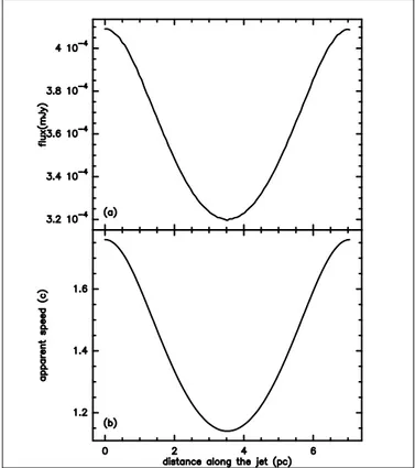
The resemblance with some observed VLBI jets is ob-vious. One interesting point to note here is that the cloud initially appears to move in a direction nearly perpendic-ular to the axis of the jet. Also, on Fig. 3, the intensity of the cloud changes dramatically along the trajectory, in contrast with the optically thick case of Fig. 2. This flux variation of the cloud is illustrated on Fig. 4 and Fig. 5. The apparent speed of the cloud is also plotted in these figures. It is always superluminal here (up to 7c in the case of Fig. 3), but more importantly it greatly varies along the trajectory.
Fig. 4. Flux and apparent speed along the trajectory for Fig. 2.
4.2. Flux of cloud
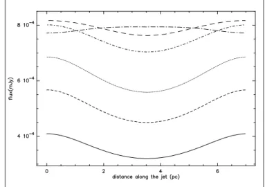
The variation of the cloud flux along the helix for different speeds is shown in Fig. 6 (α = 70◦) and Fig. 7 (α = 5◦).
Two phenomena are competing in the flux variation along the helix: the Doppler effect and the orientation of the magnetic field. The Doppler factor depends on the co-sine of the angle θ between the velocity vector and the line of sight, while the synchrotron flux depends on the sine of this same angle (because magnetic field and cloud velocity vector are parallel and both tangent to the helix, and the synchrotron intensity depends on the magnetic field
com-6 V. Despringre et al.: Two-fluid model for VLBI jets
Fig. 5. Flux and apparent speed along the trajectory for Fig. 3.
ponent which is perpendicular to the line of sight). Hence, at low speeds, the intrinsic flux is maximum where this an-gle is the largest (middle of the curves in our examples), whereas the Doppler factor creates the opposite behaviour at very high speeds. At intermediate speeds, two maxima can appear due to the two competing effects.
In the case of a large angle to the line of sight (Fig. 6), the Doppler factor is smaller than 1 (flux dimming) and decreases with increasing cloud speed (for β >∼ 0.5). Here, the effect of the magnetic field is dominated by the Doppler effect at speeds as low as β = 0.5. This is be-cause the variation of the angle θ between the magnetic field and the line of sight is small. In the opposite case (Fig. 7), the Doppler factor δ is always larger than 1 (flux amplification) and increases with the cloud speed. The ef-fect of the magnetic field is dominant at speeds as high as β = 0.96 where two maxima are present. The consequence of the competition between these two phenomena is that the flux does not simply increase with β. This is true only for a limited range of speeds and at some locations along the trajectory.
4.3. Contrast
The ratio Fmax/Fmin (that we call contrast) of the
maxi-mum to the minimaxi-mum fluxes of the cloud over one period
Fig. 6. Flux behaviour along trajectory for different speeds and α = 70◦, ν = 109
Hz: β = 0.1 (– · –), 0.5 (– – –), 0.7 (- · -), 0.9 (· · ·), 0.96 (- - -), 0.99 (——).
Fig. 7.Same as Fig. 6 for α = 5◦and ν = 1012
Hz.
of the helix, is plotted vs frequency in Fig. 8 for several speeds.
The angle of the jet to the line of sight is set to 30◦for
this figure. The contrast depends on the optical thickness of the cloud: it is higher in the optically thin regime at high frequencies. The competition between the two effects discussed in Sect. 4.2 is illustrated by the fact that the difference in this contrast between the two regimes has a minimum for β ≃ 0.7. The constrast increases with speed in the optically thick regime, but it first decreases and then increases with increasing speed in the optically thin regime.
Fig. 8.Contrast Fmax/Fminvs frequency for α = 30◦different
speeds (same as Fig. 6).
4.4. Spectra
Synchrotron spectra of the cloud at two positions distant by half a period of the helix for α = 70◦ (corresponding
to the first and fourth frame in Fig. 2) are presented in Fig. 9.
Fig. 9.Synchrotron spectra at two positions distant by half a period of the helix for α = 70◦(solid line corresponding to the
1st frame of Fig. 2, and the dotted line to the 4th frame).
At small frequencies the slope is +5/2 (the cloud is op-tically thick), and at larger frequencies, the slope is −1/2, as given by synchrotron radiation theory for a particle en-ergy distribution spectral index of 2 in the optically thin regime.
As the cloud moves along the helix, these two slopes naturally remain the same. But the transition frequency
νm, where the flux of the cloud is maximum, increases
with the projected magnetic field and the Doppler factor. The same two competing effects discussed in Sect. 4.2 are again in play here. In the case of Fig. 9, it has been shown in Sect. 4.2 that this is the Doppler effect that dominates. In general, the variation of νmalong the trajectory could
imply an apparent transition between the two regimes of optical thickness if the source is observed at a fixed fre-quency.
The influence of the particle density Neand the
mag-netic field B0 on the synchrotron spectra is shown in
Fig. 10. Increasing the particle density or the magnetic field shifts upward the optically thin part of the spectrum. The optically thick part is not sensitive to the particle den-sity, while it is shifted downward with increasing magnetic field.
Fig. 10. Influence of physical parameters on the spectrum of the blob for α = 70◦. In (a): N
e = 104 (solid line), 105
(dashed) and 106
(dotted) cm−3. In (b): B
0 = 10−3 (solid),
10−2(dashed) and 10−1(dotted) G. These spectra are for the
position where the flux is maximum (1st frame in Fig. 2)
5. Discussion and conclusion
The previous section shows that it is possible to explain observed VLBI jets with the two-fluid concept, even with a jet at rest. The presence of a relativistic ‘cloud’ (see Introduction) propagating inside the jet is the key
ingre-8 V. Despringre et al.: Two-fluid model for VLBI jets
dient in our model. We think that the idea of non- or mildly-relativistic jets in AGN and radiosources is now fully viable at all scales. It reconciles observed relativistic phenomena at scales smaller than the parsec and/or at VLBI scales, with non-relativistic jets both at large scale (observations) and at the central part of AGNs (theories of jet extraction).
The helical trajectory, observationally suggested, re-laxes the constraint on the angle between the jet and the line of sight. The consequences of curved paths of VLBI blobs have not been fully appreciated, but AGN “unifi-cation” models would certainly benefit from such consid-erations. The helical trajectory also yields the observed behaviour that the initial direction of propagation of a blob can be nearly perpendicular to the jet axis. This is observed in quite a few sources (e.g. Mrk 501, Conway & Wrobel 1995). The case of a small angle to the line of sight shown in Fig. 3 is rather reminiscent of the BL Lacertae object 0235+164 (Chu et al 1996).
From the synthesized maps, different observational quantities are presented in Sect. 4. This helps in under-standing the origin of flux variation along the trajectory. These are also observational curves that could bring some information on the different parameters of the model. Even if it requires multiepoch and multifrequency data, our model can probably be already applied in some cases. For instance, Qian et al. (1996) used a helical model to in-terpret the intrinsic evolution of the VLBI blobs in 3C345. As has been seen in Sect. 4.2, the orientation of the mag-netic field also yields a variation of the flux along the tra-jectory. This has not been taken into account by these authors, but it could lead to different results.
Naturally, the present work is very simplistic, but un-doubtly justifies sophistication of the simulations. Such simulations are necessarily limited because the reality en-compasses so many physical phenomena. The originality of our work is that no ad-hoc assumption is made in the sense that the physics of the radiating cloud can be en-tirely derived from theories of jet extraction and high-energy radiation. In the same way, the trajectory could also be precised from physical calculations. Our goal here is to build a fully physically coherent picture of AGNs from the accretion disk up to the VLBI jet, under ob-servational constraints from the radio to the high energy radiation. The next step will be the complete simulation of the stationary jet, by including the polarization with the addition of a turbulent magnetic field. In a later stage, the evolution of the cloud along its way from the region where it produces γ-rays to the VLBI scale will be theoretically studied and implemented in the numerical simulations.
Acknowledgements. We would like to thank an anonymous ref-eree for very useful comments.
References
Achatz U., Lesch H., Schlickeiser R., 1990, A&A 233, 391
Achatz U., Schlickeiser R., 1992, in:Extragalactic radio sources: from beams to jets, eds. J. Roland, H. Sol and G. Pelletier (Cambridge University Press), p. 256
Bowman M., Leahy J.P., Komissarov S.S., 1996, MNRAS 279, 899
Chu H.S., B˚a˚ath L.B., Rantakyr¨o F.T., Zhang F.J., Nicholson G., 1996, A& A 307, 15
Conway J.E., Wrobel J.M., 1995, ApJ 439, 98 Fraix-Burnet D., 1992, A& A 259, 445
Fraix-Burnet D., Pelletier G., 1991, ApJ 367, 86
G´omez J.L., Alberdi A., Marcaide J.M., 1993, A& A 274, 55 G´omez J.L., Alberdi A., Marcaide J.M., 1994a, A& A 284, 51 G´omez J.L., Alberdi A., Marcaide J.M., Marscher A.P., Travis
J.P., 1994b, A& A 292, 33
Hanasz M., Sol H., 196, MNRAS in press Henri G., Pelletier G., 1991, ApJ 383, L7
Marcowith A., Henri G., Pelletier G., 1995, MNRAS 277, 681 Pelletier G., Roland J., 1986, A& A 163, 9
Pelletier G., Roland J., 1988, A& A 196, 71 Pelletier G., Roland J., 1989, A& A 224, 24 Pelletier G., Sol H., 1992, MNRAS 254, 635
Phinney E.S., 1987, in:Superluminal Radio Sources, eds. J.A. Zensus and T.J. Pearson (Cambridge University Press), p. 301
Qian S.J., Krichbaum T.P., Zensus J.A., Steffen W., Witzel A., 1996, A& A 308, 395
Sol H., Pelletier G., Ass´eo E., 1989, MNRAS 237, 411 Vermeulen R., 1995, in:IAU Symposium 175, Extragalactic
Ra-dio Sources, (Dordrecht: Kluwer)
Zensus J.A., 1995, in:IAU Symposium 175, Extragalactic Radio Sources, (Dordrecht: Kluwer)
This article was processed by the author using Springer-Verlag LATEX A&A style file L-AA version 3.