ALGORITHM BASED FAULT TOLERANCE WITH WAVELETS
ROMAN ANDREEV
Abstract. In wavelet Galerkin discretizations of partial differential equations the value of a coefficient of the discrete solution directly translates into its importance. In the context of a parallel iterative computation on faulty computational nodes we propose to use this information to distribute the coefficients in a way that minimizes the expected loss upon hard node failure, thus dramatically increasing the chances of approaching the discretization accuracy.
1. Introduction
A parallel computation may experience hardware or software failure [3]. We focus here on the so-called hard failure of computational nodes. We devise a data allocation scheme that, based on the failure probability of those nodes, distributes the data such as to minimize the expected loss, assuming that every piece of data (item) has a certain additive importance (item value) associated with it independently of other items. This situation appears in iterative solution algorithms for linear algebraic systems arising from discretizations of partial differential equations. Changing to a wavelet basis allows to interpret each coefficient as an item and to assign an item value to it in a natural way. Thus we propose to dynamically redistribute the coefficients in the course of the iterative solution algorithm across the computational nodes in a way that minimizes the expected accuracy loss due to the potential node failure. This redistribution is an instance of algorithm based fault tolerance and complements other fault resilience techniques such as checkpointing.
In the first part we introduce our data allocation model and propose algorithms for optimizing the allocation. In the second part we present proof-of-concept numerical experiments with a wavelet discretization of a simple differential equation.
2. Data allocation model
2.1. Definitions. A collection I of items is to be stored on N nodes. With each item i we associate an item value vi ≥ 0, and set
vtot :=Pivi.
All items have the same size of one unit. The n-th node can store an integer number Cn ≥ 0 of distinct items, called the capacity of node n. We assume that each item can
be replicated and stored at any node at no cost while within the capacity. We call
1 #I(
P
nCn) − 1
the redundancy index. It is nonnegative if and only if the joint capacity of nodes is sufficient to store all items. A pure allocation map is a binary matrix A ∈ {0, 1}I×N with
the column sum Piain ≤ Cn for each node n. Let
A01:= {A = (ain)in ∈ {0, 1}I×N :Piain≤ Cn}
(1)
Date: September 4, 2016.
collect all such pure allocation maps. A node status vector is a binary vector x ∈ {0, 1}N
with the interpretation that
the n-th node is operational if and only if xn= 1.
Given a node status vector x and a pure allocation map A we call φx(A) :=Pi(1 −Qn(1 − xnain))vi
(2)
the accessible value. Note that (1 − xnain) is zero if xn = 1 and ain = 1, which means
that node n is operational and stores item i. Thus the product over n equals zero if item i is available on some node, and equals one otherwise. The accessible value φx(A) is
therefore the total value of available items, where each item is counted at most once. An alternative and sometimes more convenient way to write the product in the definition of φx(A) for binary x and A is Qn(1 − xnain) =Qn(1 − xn)ain, where 00 := 1.
We extend φx(A) as defined in equation (2) to a function on x ∈ RI and A ∈ RI×N in
the obvious multiaffine way, so that φx(A) is affine in each column of A. By nonnegativity
of the item values, φx(A) is nondecreasing in x and in A in the sense that φx(A) ≥ φy(B)
whenever A ≥ B and x ≥ y componentwise. Let A := convA01 denote the closed convex
hull of A01⊂ RI×N. A point in A is called a mixed allocation map.
2.2. Allocation optimization. We suppose now that x above is a vector of independent binary random variables with probabilities pn := P[xn = 0] and ˆpn:= P[xn = 1] = 1 − pn.
In particular E[xn] = ˆpn. We refer to pnas the failure probability of node n. Given A ∈ A,
¯
φ(A) := E[φ(·)(A)] =
P
i(1 −
Q
n(1 − ˆpnain))vi
is the expected accessible value. Observe that ¯φ is multilinear and nonnegative on A, and ¯
φ(0) = 0. We can now formulate the allocation problem:
Find some A ∈ A01 s.t. φ(A) ≥ ¯¯ φ(B) ∀B ∈ A.
Alternatively, one can minimize the expected loss ¯
ψ(A) := PiviQnpanin,
which is related to the expected accessible value by ¯φ + ¯ψ = vtot for pure allocation maps
A ∈ A01. Since the solution may not be unique, the problem could be supplemented
by the proximity condition that the number of differing entries |Aref − A|0 for a given
Aref ∈ A01 be minimal, or relaxed to argminA∈A01{ ¯φ(A) + γ
1
p|Aref − A| p
p}, where | · |p
denotes the vector p-norm of all entries (neither condition guarantees uniqueness). 2.3. Case of two items. Suppose #I = 2. We can assume that each node has capacity Cn = 1, excluding uninteresting cases. Assume also vi = 1 for the item values. A
pure allocation map that minimizes the expected cost is then determined by its first row a ∈ {0, 1}N, the second one being the complementary b := 1 − a, so that we can write
¯
ψ(a) = pa+ pb using the multiindex notation. Setting α := pa and β := pb, observe that
the product αβ is independent of a. This implies that the correspondence (α + β) 7→ | log(α/β)| is nondecreasing. Consequently, minimizing ¯ψ(a) = α + β is equivalent to minimizing | log(α/β)| = |S1− S0|, where S1 =Pnanlog pn and S0 =Pn(1 − an) log pn,
over a ∈ {0, 1}N. This is the optimization version of the set partition problem, which is
2.4. Case of two nodes. The case N = 2 of two nodes can be treated explicitly. By symmetry suppose 0 < p1 ≤ p2 < 1 for the failure probabilities. Let vσ(1) ≥ vσ(2) ≥
. . . ≥ vσ(#I) be a nonincreasing rearrangement of the item values. If an allocation map
A ∈ A01 is a minimizer of the expected loss ¯ψ, the capacity Cn=
P
iain of each node is
exhausted, and (Cn− C12) items are stored on node n only, where C12 ≥ 0 is the number
of shared items that are stored on both nodes. For any fixed number C12 of shared items,
the allocation map A with rows (1) ai = (1, 1) for 1 ≤ σ(i) ≤ C12,
(2) ai = (1, 0) for C12< σ(i) ≤ C1,
(3) ai = (0, 1) for C1 < σ(i) ≤ C1+ C2− C12,
(4) ai = (0, 0) else,
minimizes the expected loss ¯φ(A) =PiviQnpanin, as can be seen with the rearrangement
inequality and p1p2 ≤ p1 ≤ p2 < 1. Increasing C12 by one decreases the expected loss by
the amount (1 − p2)(p1vσ(C12+1)− vσ(C1+C2−C12)), which is nonnegative as long as
p1vσ(C12+1) ≥ vσ(C1+C2−C12).
(3)
Once this condition is violated, it remains false by the monotonicity of vσ(·). We arrive
at the following algorithm for finding an optimal pure allocation map for two nodes: (1) Initialize C12= min{max{C1+ C2− #I, 0}, #I}.
(2) While C12 < min{C1, C2} and condition (3) is satisfied: Increase C12 by one.
(3) Construct A as above.
We remark that the algorithm does not require Cn≤ #I or #I ≤ C1+ C2.
2.5. Pairwise optimization. One might attempt to minimize the expected loss ¯ψ(A) by optimizing A node by node, but it is more effective to optimize over pairs of nodes:
(1) Let an initial guess A ∈ A be given. (2) Repeat:
(a) Choose two nodes n1 6= n2 uniformly at random.
(b) Update the columns n1 and n2 of A using the two node optimization
proce-dure with the effective item weights ˜vi := vi
Q
n /∈{n1,n2}p
ain
n .
Once each node has been selected, the current allocation map A will necessary be a pure allocation map that exhausts the node capacities, even if the initial guess was not a pure allocation map. The optimization process can be stopped as soon as the value of ¯ψ(A) stabilizes, but for simplicity, in the experiments below we always perform exactly 100 iterations (observed to be more than sufficient) starting with the zero allocation map.
In a (near-)optimum solution the most reliable nodes tend to store the most valuable items. The random pair selection step could therefore be replaced by a systematic process which proceeds from the most reliable to the least reliable nodes starting with the zero allocation map. In a similar vein, the likelihood of a random selection of a pair of nodes could be anticorrelated with the probability of their simultaneous failure.
3. Application to wavelet discretization
3.1. Model problem. As a model problem we take the elliptic equation u′′ = 1 on the
unit interval (0, 1) with zero Dirichlet boundary conditions. The problem is discretized with P1 finite elements (hat functions) on an equidistant mesh consisting of 210
subin-tervals. This leads to the algebraic equation Au = f , where the boundary degrees of freedom have already been eliminated. Now we suppose we have a wavelet basis [2] at hand that forms a Riesz basis in H1 (we will use the heuristic wavelet construction from
[1] with a slight adaptation to the boundary conditions). Let T denote the matrix such that waveleti =
P
kTikhatk, or in other words, TT applied to a vector of multiscale
coefficients yields a vector of single scale coefficients. By the Riesz basis property, the matrix TATT is well-conditioned uniformly in the discretization level. Thus we consider
the convergent stationary Richardson iteration
wℓ+1 = wℓ+ (Tf − TATTwℓ), w0 := 0,
(4)
where wℓ is the vector of coefficients of the ℓ-th iterate uℓ ≈ u with respect to the
wavelet basis. Specifically, we scale the wavelet basis such that the contraction factor is ρ(I − TATT) = 0.95, which entails an error reduction factor of about 0.95100 ≈ 0.006
every 100 iterations, cf. Figure 1. Much lower contraction factors are in fact possible but we wish to simulate here a more general situation.
We consider the following model scenario. Suppose the iterate wℓ is distributed across
N computational nodes. We wish to perform one Richardson iteration, but some of the nodes might fail in the process and corrupt the accuracy (measured in the H1semi-norm).
How should we distribute the coefficients such as to minimize the loss of accuracy? To that end we interpret the coefficients as data items and use the Riesz basis property to interpret vi := |(wℓ)i|2 as the item value of the i-th coefficient.
3.2. Numerical experiments. We use the pairwise optimization algorithm from Sec-tion 2.5 in each Richardson iteraSec-tion to determine an allocaSec-tion map. The wavelet coeffi-cients which are not covered by the allocation map after a possible simulated node failure are set to zero. The failure probability pn of the n-th node during one Richardson
itera-tion is fixed at the beginning of the iteraitera-tion as a random number distributed uniformly between 1% and 2%. We perform 105 Richardson iterations for different number of nodes
N with different capacities Cnto obtain statistics on the error eℓ := |u−uℓ|H1. The
capac-ities are determined through the redundancy index r by setting Cn:= (1+r)⌈(210+1)/N ⌉
for each node. We vary N = 2, 4, 8, and 2r = −1, 0, 1, 2, . . .. If N = 2 then only r ≤ 1 is meaningful.
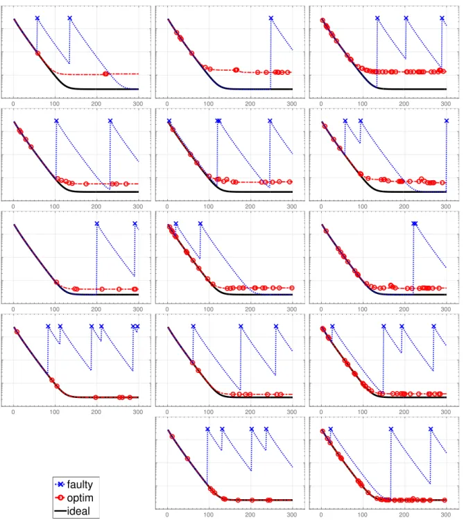
In Figure 1 we document the error eℓ during the first 300 Richardson iterations. Each
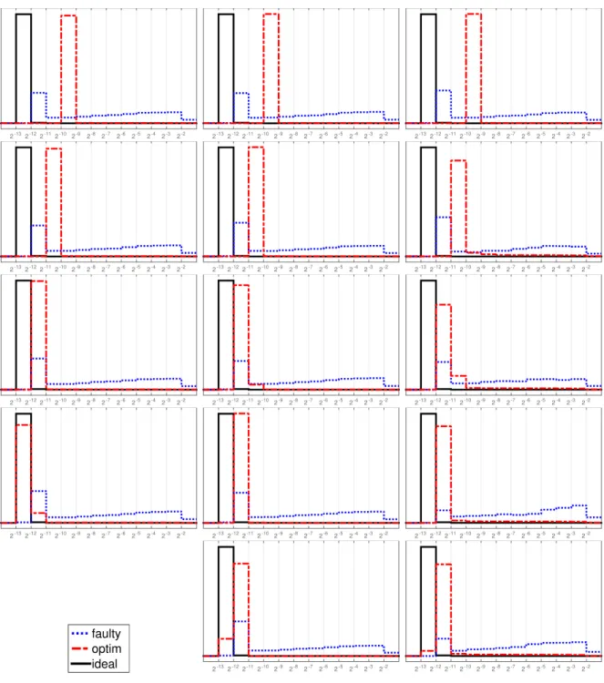
plot contains the runs a) without node failure, b) on one faulty node of sufficient capacity, and c) on N nodes with the optimized allocation. These are labeled “ideal”, “faulty”, and “optim”, respectively. We see that the optimization strategy, even if the redundancy index is negative, allows to greatly reduce the loss of accuracy at the cost of a slightly elevated error as ℓ → ∞. Figure 2 documents the distribution of the error for the same runs over 105 Richardson iterations and shows that the optimized allocation forces the
error to hover close to the discretization error, whereas the error is typically much larger in the single faulty node scenario. Increasing the number of nodes (for the same redundancy index) slightly increases the error of the optimized strategy because node failure becomes slightly more likely. Increasing the redundancy index (for the same number of nodes) strongly decreases that error and practically recovers the ideal faultless situation.
4. Conclusions
Under idealized assumptions such as negligible node to node communication cost and uniform data item size, we have developed a framework for data redistribution across faulty computational nodes with the aim of minimizing the expected data loss under potential node failure. We have then proposed and illustrated the notion that wavelet discretizations of partial differential equations naturally fit that framework and thus induce algorithm based fault tolerance.
5. Acknowledgment
Supported by French ANR-12-MONU-0013 and Swiss NSF #164616. References
[1] Roman Andreev. Wavelet-in-time multigrid-in-space preconditioning of parabolic evolution equations. SIAM J. Sci. Comput., 38(1):A216–A242, 2016.
[2] Wolfgang Dahmen. Wavelet and multiscale methods for operator equations. In Acta numerica, 1997, volume 6 of Acta Numer., pages 55–228. Cambridge Univ. Press, Cambridge, 1997.
[3] Ifeanyi P. Egwutuoha, David Levy, Bran Selic, and Shiping Chen. A survey of fault tolerance mech-anisms and checkpoint/restart implementations for high performance computing systems. J. Super-comput., 65(3):1302–1326, 2013.
(R. Andreev) Universit´e Paris Diderot, Sorbonne Paris Cit´e, LJLL (UMR 7598 CNRS), F-75205 Paris, France
0 100 200 300 0 100 200 300 0 100 200 300 0 100 200 300 0 100 200 300 0 100 200 300 0 100 200 300 0 100 200 300 0 100 200 300 0 100 200 300 0 100 200 300 0 100 200 300 faulty optim ideal 0 100 200 300 0 100 200 300
Figure 1. Estimated error |u−ui|H1 as a function of the iteration number
1 ≤ i ≤ 300, for ideal, faulty, and optimized computation. The vertical logarithmic scale ranges from 10−4 to 1. Crosses/circles indicate node
fail-ure. The optimized computation is performed on N = 2, 4, 8 nodes (→) with redundancy index r given by 2r = −1, 0, 1, 2, 3 (↓).
2-132-122-112-102-9 2-8 2-7 2-6 2-5 2-4 2-3 2-2 2-132-122-112-10 2-9 2-8 2-7 2-6 2-5 2-4 2-3 2-2 2-132-122-112-10 2-9 2-8 2-7 2-6 2-5 2-4 2-3 2-2 2-132-122-112-102-9 2-8 2-7 2-6 2-5 2-4 2-3 2-2 2-132-122-112-10 2-9 2-8 2-7 2-6 2-5 2-4 2-3 2-2 2-132-122-112-10 2-9 2-8 2-7 2-6 2-5 2-4 2-3 2-2 2-132-122-112-102-9 2-8 2-7 2-6 2-5 2-4 2-3 2-2 2-132-122-112-10 2-9 2-8 2-7 2-6 2-5 2-4 2-3 2-2 2-132-122-112-10 2-9 2-8 2-7 2-6 2-5 2-4 2-3 2-2 2-132-122-112-102-9 2-8 2-7 2-6 2-5 2-4 2-3 2-2 2-132-122-112-10 2-9 2-8 2-7 2-6 2-5 2-4 2-3 2-2 2-132-122-112-10 2-9 2-8 2-7 2-6 2-5 2-4 2-3 2-2 faulty optim ideal 2-132-122-112-10 2-9 2-8 2-7 2-6 2-5 2-4 2-3 2-2 2-132-122-112-10 2-9 2-8 2-7 2-6 2-5 2-4 2-3 2-2
Figure 2. Distribution of the error (as in Figure 1) over 105 Richardson
iterations. The bins are delimited by 2−13, 2−12, . . . , 2−2, the area under
each curve equals 100%.