Certified Detection of Parallel Robot Assembly Mode under Type 2 Singularity Crossing Trajectories

HAL Id: hal-01435808

https://hal.archives-ouvertes.fr/hal-01435808

Submitted on 24 Jun 2019

HAL is a multi-disciplinary open access

archive for the deposit and dissemination of

sci-entific research documents, whether they are

pub-lished or not. The documents may come from

teaching and research institutions in France or

abroad, or from public or private research centers.

L’archive ouverte pluridisciplinaire HAL, est

destinée au dépôt et à la diffusion de documents

scientifiques de niveau recherche, publiés ou non,

émanant des établissements d’enseignement et de

recherche français ou étrangers, des laboratoires

publics ou privés.

Certified Detection of Parallel Robot Assembly Mode

under Type 2 Singularity Crossing Trajectories

Adrien Koessler, Alexandre Goldsztejn, Sébastien Briot, Nicolas Bouton

To cite this version:

Adrien Koessler, Alexandre Goldsztejn, Sébastien Briot, Nicolas Bouton.

Certified Detection of

Parallel Robot Assembly Mode under Type 2 Singularity Crossing Trajectories. 2017 IEEE

Inter-national Conference on Robotics and Automation (ICRA 2017), May 2017, Singapour, Singapore.

�10.1109/ICRA.2017.7989720�. �hal-01435808�

Certified Detection of Parallel Robot Assembly Mode under Type 2

Singularity Crossing Trajectories

Adrien Koessler

, Alexandre Goldsztejn

, S´ebastien Briot

and Nicolas Bouton

Abstract— Increasing the size of operationnal workspace is one of the main problems parallel robots are faced with. Among all the proposed solutions to that, crossing Type 2 singularities using dedicated trajectory generation and multi-model controller has a great potential. Yet, this approach is not sufficient for the robot to operate autonomously, as assembly mode detection during the motion currently requires additional redundant information.

To tackle this problem, we propose an algorithm based on Interval Analysis (IA) that is able to track the end-effector of the robot even under assembly mode change. IA-based solvers for the forward kinematic problem of parallel robots are well known, but they cannot be used under assembly mode change. Compared to those classical approaches, the major modification introduced is the tracking of end-effector velocity in addition to its pose. Using this new information of velocity, the algorithm is capable to monitor the assembly mode change of the robot happening when the singularities are crossed. The behavior and the reliability of this algorithm are analyzed experimentally on a five-bar planar parallel mechanism.

I. INTRODUCTION

It is acknowledged that parallel manipulators have advan-tages in terms of rigidity, cycle time and payload-to-weight ratio over their serial counterparts. Yet, their workspace is usually split into several assembly modes separated by Type 2 (or parallel) singularities [1][2].

These are difficult to deal with as one (or more) manipu-lator’s degree of freedom becomes uncontrollable. Assembly modes separated by Type 2 singularities cannot be inter-connected to each other using classical control algorithms, resulting in a decrease in the size of the operationnal workspace.

Therefore, approaches leading to operationnal workspace enlargement have been developed, such as:

• Optimal design of parallel manipulators to maximize the size of the operationnal workspace [3] or to eliminate Type 2 singularities [4][5]

• Redundantly actuated robots [6][7], which is a costly solution or robots with variable actuation modes [8][9] • Assembly mode changing trajectories based on cusp

points detection [10]

• Dedicated trajectory generation and control to cross directly the singularity locus [11][12]

The latter approach seems more versatile to us, as it can be generalized to any type of parallel robot. It emerged with the

1 _{Universit Clermont Auvergne, CNRS, SIGMA Clermont,}

Institut Pascal, F-63000 Clermont-Ferrand, France {Adrien.Koessler, Nicolas.Bouton}@sigma-clermont.fr

2 _{Laboratoire des Sciences du Num´erique de Nantes (LS2N),}

UMR CNRS 6004, 44321 Nantes, France {Alexandre.Goldsztejn, Se-bastien.Briot}@ls2n.fr

discovery of a physical criterion allowing the non-degeneracy of the manipulator’s dynamic model in Type 2 singular configurations [11]. Using this criterion, trajectory plan-ners and dedicated multi-model Computed Torque Control schemes [13][14] have been developed and tested, proving their efficiency in most cases. Nevertheless, unavoidable tracking errors with respect to this desired trajectory can have a strong impact in the vicinity of the singularity, up to missing the assembly mode change. Hence monitoring the assembly mode during the robot motion is needed.

Methods to detect the assembly mode of a robot have already been investigated. The introduction of measurement redundancy (using passive instrumented legs or encoders in passive joints) allows to achieve it, but the placement of encoders needs to be chosen carefully [15]. External measurement with vision, either to monitor directly the pose of the platform [16] or the orientation of the legs of the mechanism [17], has also been investigated. Both of those approaches come at an extra cost and might be difficult to integrate in an industrial environment.

An interesting alternative is based on interval analysis. IA is a field of mathematics that treats variables as intervals, meaning that the variable’s value must lie between the lower bound and the upper bound of the interval [18]. Thus, it can be very useful for reliable computations in bounded-error context. Numerous applications of IA can be found in robotics [19] and control, such as mobile robot localization [20][21], robot kinematic calibration [22], robust control [23], positioning precision analysis and synthesis [24][25]. In parallel robotics in particular, methods to compute the aspects of the workspace have been discovered [26] [27].

Merlet has applied IA to solve the Forward Kinematic (FK) problem of a Gough-Stewart platform [28], using the equations of the inverse kinematics and a start point. Thanks to constraint propagation techniques, his algorithm showed ability to distinguish the different solutions of FK problem even when the platform is close to Type 2 singularities. Such a technique, which is time-efficient and does not require additional sensors, is highly interesting in an industrial context. Yet it has to be adapted to assembly mode changing detection, as it does not handle it: if the robot reaches a Type 2 singularity and exits it, the algorithm will compute enclosures of the pose that diverge, and therefore will not be able to state in which assembly mode it exited [28].

Hence, our goal is to provide an IA-based algorithm that is able to track the assembly mode of a robot attempting to cross Type 2 singularities.

Notations: In the following, bracketed symbols are used to denote interval enclosures of the corresponding quantities. For instance, a scalar a ∈ R car be enclosed by the interval [a] = [a, a] ∈ IR such as a ≤ a ≤ a, where IR is the set of scalar real intervals. An interval vector is the cartesian product of the scalar interval of each component. For in-stance, a vector p= (p1 · · · pn)T _{∈ R}n _{admits a bracketing} [p] = [p

1, p1] × · · · × [pn, pn] ∈ IR

n_{. This explains why a} vector of intervals is generally called a box.

II. POSE AND VELOCITY TRACKING ALGORITHM A. Kinematic modelling of parallel mechanisms

This section aims to briefly recall the kinematic equations of a parallel manipulator with n degrees of freedom and driven by n actuators. The position and the speed of the manipulator can be fully described using:

• q and ˙q that represent respectively the vector of active joints variables and active joints velocities,

• x and ˙x that are the end-effector pose parameters and their derivatives with respect to time, respectively. In the following, the sampling time is ts with time step k, while x_k= x(kts), ˙xk= ˙x(kts), qk= q(kts) and ˙qk= ˙q(kts).

The loop-closure equation of the mechanism can then be written as [29]:

f(x, q, ξξξ ) = 0 (1)

where ξξξ is the vector of geometrical parameters. The first-order kinematic equation is:

Jx(x, q, ξξξ ) ˙x + Jq(x, q, ξξξ ) ˙q = 0 (2) where Jx and Jq are the (n × n) Jacobian matrices of the robot.

B. Outline of the algorithm

Tracking the pose given joint values information ˆqk is usually done by solving (1) using a local solver, usually a Newton method, and the previous pose as initial condi-tion. This is however unreliable, especially near singularities (See [29], chapter 4). IA gives rise to a reliable variant of this tracking process [28]: Given an enclosure [q]k on the joint coordinates at step k, one can compute an enclosure [x]k of the pose solving (1) with an IA-based solver. Merlet [28] also proposed to use the previous pose enclosure[x]k−1 and an upper bound on the speed of the end-effector, given here under the form of an enclosure of all possible speed vectors [vmax] ∈ IRn_{, to obtain an initial domain[x]kfor the IA-based} solver:

xk= xk−1+

Z ts

0 v(t) dt ∈ [x]k−1+ ts[vmax] =: [x]k. (3) This initial domain drastically simplifies and speeds up the solving process, since it is usually quite small and contains only the solution corresponding to the tracked trajectory. As mentioned in the previous section, this IA-based tracking process fails and computes divergent enclosures in the vicin-ity of singularities [28]. f1 f2 i X Y O

Fig. 1: An example of crossing attempt. i is the initial configuration, f are the possible final configurations. The dotted line represents the singularity locus, the arrows the possible trajectories.

We propose here to extend this IA-based tracking process by tracking the end-effector velocity in addition to its pose. Using the end-effector velocity information, we might be able to tell in which assembly mode the robot has exited the singularity. For instance, imagine that the robot’s end-effector follows a path intersecting a Type 2 singularity; it may cross the singularity or ”bounce” on it. If we add the information that the speed along this path did not change its sign during the whole transfer, it is obvious that the robot didcross the singularity. This is the type of information that we need to create within our algorithm.

An example is shown on Fig. 1. With the knowledge that the end-effector only had negative velocity along the Y -axis, the only feasible final configuration is f2.

The end-effector speed is tracked similarly to its pose. An initial domain for the end-effector velocity at step k is computed using the enclosure at step k − 1 and a given maximal acceleration[amax] ∈ IRn_:

˙xk= ˙xk−1+

Z ts

0 a(t) dt ∈ [˙x]k−1+ ts[amax] =: [˙x]k. (4) This enclosure can be safely intersected with [vmax]. Then using an enclosure [ ˙q]k of the joint velocity, this initial domain is sharped by solving (2) using an IA-based solver. In fact, this velocity enclosure can be used to improve the initial pose enclosure (3): Since 0 ∈[amax] we have ts[amax] = [0,ts][amax], and therefore for all t ∈ [(k − 1)ts, kts]

˙x(t) = ˙xk−1+

Z t

0 v(t) dt ∈ [˙x]k−1+ [0,ts][amax] = [˙x]k, (5) i.e., the end-effector velocity enclosure (4) at time kts is actually an enclosure of the velocity for all t ∈[(k − 1)ts, kts]. As a consequence, (3) can be improved as follows:

[x]k:= [x]k−1+ ts[˙x]k. (6) As previously, the solver will fail sharpening the initial end-effector pose and velocity domains in the vicinity of singularities, since the matrix Jx in (2) is ill-conditionned. Thus, in such configurations, the maximal acceleration is the

only information that can be used to enclose the end-effector velocity. It follows from (4) that the width of its enclosure will grow approximately as k tsk[amax]k. Despite its constant growth, it is expected that the velocity enclosure will give enough information to remove all the parasite solutions to the FK problem, thus allowing to detect the current assembly mode. For instance, in the situation of Figure 1, the end-effector velocity enclosure can remain negative in spite of its constant growth during the singularity crossing provided that the speed is high enough.

C. Description of the algorithm

Algorithm 1 provides the pseudo-code of the end-effector pose and velocity tracking algorithm. The procedure read reads measurement of the joint coordinate and velocity (the latter being usually approximated using possibly filtered finite differences). It returns true in case of successful acquisition, false otherwise when the motion is finished. The procedure contract uses standard IA-based algorithms (numerical constraint propagation, including the interval Newton and the interval Gauss-Seidel operators [18], the forward-backward contractor [30], etc.) in order to contract the domains [x]k and [˙x]k subject to the given constraints. The domains[ξξξ ], [εεεq] and [εεε˙q] are considered as parameters of the constraint system and are not contracted.

The inputs of the algorithm are:

• The kinematic model f, from which are computed the derivatives Jx and Jq. These expressions are suitable to perform interval evaluations and numerical constraint programming.

• Interval enclosures [x]0 and [˙x]0 of the initial end-effector pose and velocity.

• Upper bounds on the end-effector velocity and accel-eration given under the form of interval enclosures [vmax] and [amax] of all possible end-effector velocity and acceleration vectors.

• An enclosure[ξξξ ] of the geometric parameters.

• The joint and joint velocity measurement error bounds [εεεq] and [εεε˙q], given under the form of intervals which contain all possible errors.

• The sampling time ts.

Provided that the initial enclosure and the bounds involved in the algorithm are valid, the IA-based constraint solving process ensures that the true end-effector pose and velocity are enclosed correctly for all times. The next section discuss in detail the DexTAR parallel robot, its model and the bounds that will be used in the experiments.

III. CASESTUDY:ASSEMBLY MODE CHANGE OF A FIVE-BAR ROBOT

A. Robot kinematic analysis

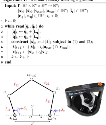
For the purpose of the experiments, a five-bar planar parallel robot is used: the DexTAR, manufactured by the company Mecademic. The design of the robot is described in [3]. A picture of the robot and a scheme are presented in Fig. 2. It exhibits the two joint inputs q1, q2 (corresponding to motors located at A1, A2) and the seven geometrical

Algorithm 1: Pose and velocity tracking algorithm Input: f : Rn_{× R}n_{× R}m_{→ R}n_; [x]0, [˙x]0, [vmax], [amax] ∈ IRn;[ξξξ ] ∈ IRm; [εεεq], [εεε˙q] ∈ IRn_{; t} s> 0; 1 k← 0; 2 while read( ˆqk, ˆ˙qk) do 3 [q]k← ˆq_k+ [εεεq]; 4 [ ˙q]k← ˆq_k+ [εεεq];

5 constract[x]k and[˙x]k subject to (1) and (2); 6 [˙x]k+1← ([˙x]k+ ts[amax]) ∩ [vmax]; 7 [x]_k+1← [x]_k+ t_s[x]_k; 8 k← k + 1; 9 end A1 q1+δ1 A2 q2+δ2 B1 B2 E(x, y) `11 `12 `22 `21 d X Y O

Fig. 2: DexTAR geometry

parameters taken into account: five lengths`11,`21,`12,`22, d and two angular offsets δ1, δ2. The output is the motion of the end-effector E, described by the pose x= (x y)T _and the velocity ˙x= ( ˙x ˙y)T_.

The system of equations for geometric loop closure (1) is given by, for i= 1, 2:

fi= (x ± d

2− `i1cos(qi1))

2_{+ (y − `i1sin(qi1))</sub>2<sub>− `}2

i2= 0. (7) Enclosures[ξξξ ] of the values of the geometrical parameters ξ

ξ

ξ are obtained through calibration procedure. It is performed using a Leica AT901 laser tracker. The adapted DETMAX algorithm described in [31] gave the 50 optimal poses to be used for calibration. Using a least-square routine [32], estimated values ˆξiwere obtained for parameters. Under the assumption that the measurement noise is white and that the identification matrix is deterministic, an estimate ˆσi of the standard deviation of each paramenter was also computed.

TABLE I: Geometrical parameters values ξi unit [ξi] nominal `11 mm [89.832,89.995] 90 `21 mm [89.929,90.115] 90 `12 mm [89.899,90.050] 90 `22 mm [89.877,90.084] 90 d mm [117.843,118.107] 118 δ1 rad [-0.004,0.004] 0 δ2 rad [-0.004,0.004] 0

For every parameter ξi, the interval [ξi] = [ ˆξi− 5 ˆσi; ˆξi+ 5 ˆσi] was consequently set. Nominal values and parameter intervals are presented in Table I.

Daney remarked that such a result can be rigorously verified by using a purely geometric IA-based solver [33]. If the interval [ξi] are valid, it is ensured that the enclosure [x] computed by (1) cannot be equal to the empty set at any point of the trajectory. Sweeping the whole workspace (singularity locus included), we verified it was never the case in our application, thus validating the presented results.

Determining the bounds[vmax] and [amax] is by far the most challenging problem in relation with our algorithm. To the best of our knowledge, no method exist to determine the full-cycle maximum values of end-effector velocity and acceler-ation for parallel mechanisms, as the problem degenerates in Type 2 singular configurations. For our experimentations, the real value of end-effector acceleration norm k¨xkmax is monitored using an inertial unit, so that an upper bound for end-effector acceleration can be deduced. The maximal ac-celeration measured during the three experiments presented in the next section are respectively 65.5 m · s−2_{, 79.9 m · s}−2 and 50 m · s−2. The bounds [amax] chosen are respectively [−80, 80] × [−80, 80], [−80, 80] × [−80, 80] and [−70, 70] × [−70, 70]. We have no information of the maximal speed, and have used[vmax] = [−∞, +∞] × [−∞, +∞] in all experiments, showing that this information is not crucial for the success of the IA-based tracking.

Finally, the homing process of the DexTAR gives rise to [x]0 = [0.07, 0.110] × [0.048, 0.088] (m) and [˙x]0 = [−0.1, 0.1] × [−0.1, 0.1] (m · s−1_{). The sampling time is t}

s= 0.001s and [εεεq] = [− π 34000, π 34000] × [− π 34000, π 34000] (rad) is given by the coder precision. The joint velocity is classically approximated by a finite difference ˆ˙qk= ˆqk− ˆq_tsk−1 with error bound [εεε˙q] =2[εεεq]

ts .

B. Trajectory Generation and Control

As the goal is to cross Type 2 singularities to perform our tests, an adapted controller is needed. The choice we made is the trajectory generator and the multi-model Computed Torque Controller (CTC) developed by Pagis in [13].

Adapting CTC schemes to singularity crossing is tricky, since it relies on the inverse dynamic model (IDM) which degenerates in Type 2 singularities. Yet, a physical criterion can be used to keep the model consistent. It states that the acceleration undergone by the robot’s end-effector must be normal to the direction of the uncontrolled motion of the end-effector. The reader is referred to [11] for comprehensive discussion about this criterion.

This result was used by Pagis [13] to create a trajectory generator dedicated to crossing Type 2 singularities. In addition, a multi-model computed torque control scheme was created by the same author, in which a nondegenerating expression of the IDM is used in the neighbourhood of the singularity locus. Complete information can be found in [34]. This control algorithm, left unmodified, is implemented in Matlab/Simulink development environment. A Quanser

Q-PID FPGA is used to run the control programs and to communicate with the robot.

IV. EXPERIMENTS A. Tracking Algorithm Implementation

The algorithm is implemented in C++ language and com-piled using MinGW. The program uses the IBEX library [35] to perform interval computations. Experiments were carried out on a quad-core Intel i7 processor at 2.40 GHz.

Contractors are also implemented by IBEX. (7) is solved using the composition Cf of a Newton iteration [36] (CtcNewton) and a Forward-Backward contractor (CtcFwdBwd) based on HC4revise algorithm [30]. The velocity equation is implemented through symbolic differen-tiation of (7), and related contractor CJ is obtained through an interval Gauss-Seidel method (See [18], Chapter 7). Cf and CJ are composed and iterated using CtcFixPoint contractor. Experiments proved those choices to be simple and time-efficient: more advanced algorithms as Acid or shaving operators did not improve the contraction.

B. Algorithm Behaviour

The first experiment consists in tracking a straight tra-jectory. It gives a good insight on the way the algorithm operates.

In this experiment, the desired trajectory crossing Type 2 singularity locus is directed along negative Y -axis of the plane represented in Fig. 2. Fig. 3 shows the end-effector pose enclosures[x]k. When approaching the singularity locus, the enclosures tend to become loose. For a short time after the crossing, the enclosures [x]k contains both solutions to the FK problem. Afterwards, the width of the boxes shrink rapidly due to an efficient contraction of the IA-based solver and the new assembly mode change is detected.

The fact that the assembly mode is detected can be explained from velocity information, as said in section II. Fig. 4 explains it: It displays the enclosure of the end-effector velocity ˙yalong the Y -axis, and its integral

∆y(k) =

Z kts

kits

˙

y(t)dt (8)

where ki= 12000 is the time step when the crossing trajec-tory begins. ∆y represents the displacement that is undergone by the end-effector. The figure shows that at time step k= 12103, when the pose boxes shrink, the real displacement value lies in ∆y(k) = [−205.4, −57.0] (mm). This allows to eliminate the possible FK solution corresponding to assembly mode 1, whose estimated displacement is only −31.3 mm using nominal values for ξξξ .

Fig. 5 shows the sizes of each interval during the crossing phase. It can be seen that all intervals grow before and right after the crossing. Still, a contraction occurs when the singularity is crossed, and the intervals locally shrink, most notably the interval[x]. The explanation is geometrical: in a singular configuration, the distal elements 12 and 22 are fully stretched along the x-axis, thus the interval on

New Assembly Mode Detected Boxes Containing Both FKP Solutions Motion Direction Singularity Locus y (m) 0.14 0.12 0.10 0.08 0.06 0.04 0.02 x (m) -0.02 0 0.02

Fig. 3: Pose boxes[x] along the trajectory, reliably enclosing the real pose of the end-effector

this coordinate gets tiny. The shrinking on other intervals arises from the couplings during the contraction phase, as the tightened interval[x] is used to contract the others. After some time, a sudden decrease in interval widths is observed: This corresponds to the moment when the algorithm has found the right solution to the FK problem.

Out of 20 tries, the average execution time of the algorithm is 5.97 s for a 6.66 second long trajectory, on an off-line implementation. This execution time is encouraging for a real-time application.

C. Algorithm operating range

When a singularity is crossed successfully by the robot, there are two outputs possible for the algorithm: either it states that the assembly mode has changed, or it cannot state on the assembly mode. Of course, the second case does not give useful information on the behavior of the manipulator. During the tests, it has been observed that the algorithm often falls into the second case when playing slower trajectories.

To prove this, several trajectories are created and played by the robot. They all follow the same path as in the previous experiment and they all succeed in crossing the Type 2 singularity. However, their respective desired velocity at singularity vsingdiffers. The outputs for our experiment are the maximal widths of[x] and [˙x] along the whole trajectory, respectively denoted by mx and m˙x. They are shown in Table II. It is also mentioned if the algorithm was able to detect the change in assembly mode.

Results show that the faster the trajectory, the tighter the intervals, both for pose and velocity. It also tends to

TABLE II: Operation range experiment result vsing(m/s) 1.458 1.354 1.264 1.185 1.053

mx(mm) 47.18 49.15 53.45 178.30 178.23

mx˙(m/s) 4.248 4.440 4.746 517.51 455.98

AM detected? yes yes yes no no

confirm the point that was made to conclude Section II-B: Faster trajectories are more likely to get their assembly mode change detected. The explanation is that at slow crossing speeds, more time is spent around the singularity, where the algorithm is unable to contract the intervals. Thus,[˙x] grows at the rate k tsk[amax]k so that [∆y] contains both solutions to FK problem, making it impossible to conclude on the assembly mode like it was done in section IV-B.

The behaviour of the algorithm has to be explained in the case where the new assembly mode is never detected. The result for the slowest trajectory is plotted on Fig. 6. It confirms that the boxes [x] grow up to the geometrical limits of the five-bar mechanism, always enclosing the two different solutions to the direct geometric problem. Boxes [˙x] are not shown for concision matters, but they follow a simple behaviour in that case: they grow up to infinity at the rate amax, since no contraction is occuring anymore. D. Reliability and eventual false positives

It was already mentionned that using valid bracketings for all the parameters, the algorithm should give reliable enclosures on x and ˙x. Two cases have been observed: either the enclosure only contains one solution to the FGM, or it contains both. The goal of this experiment is to prove that the enclosures remain reliable even in a case of failed crossing trajectory.

We define as false positive the fact that the algorithm states that a crossing attempt succeeded whereas it failed in reality. This is the worst situation that can exist, as the supervision of the robot will wrongly think that the robot is operating normally. To test this, we add an overconstraint on the torque output of the control scheme, despite using a trajectory that respects the crossing criterion. It results in an unsuccessful crossing attempt where the end-effector of the robot appears to bounce on the singularity locus.

The result is presented on Fig. 7, where the robot fails to cross the singularity. It can be seen that the algorithm keeps choosing the right solution to the FK problem (that is, the one above the singularity locus), i.e. it keeps track of the end-effector pose, thus certifying the reliability of our algorithm: no false positive was detected.

V. CONCLUSION

In order to enlarge the reachable workspace of parallel robots and to improve their reconfigurability, several methods have been developed. Using dedicated motion generators and control algorithms to cross Type 2 singularities is an interesting solution to this problem, as it can be widely generalized to all robots. However, the robot is not aware of which assembly mode it is currently in, limiting its autonomy.

(a) Velocity enclosure[ ˙y] along the trajectory. (b) Displacement enclosure[∆y] along the trajectory.

Fig. 4: Velocity information. The exact singular configuration is denoted by the solid black line.

(a) Pose intervals widths. (b) Velocity intervals widths.

Fig. 5: Interval widths during singularity crossing. The exact singular configuration is denoted by the solid black line.

An algorithm that is able to solve this problem is proposed. As IA-based FK solvers cannot deal with singularity cross-ing, end-effector velocity tracking was introduced, allowing the algorithm to successfully detect assembly mode change. The reliability of the algorithm has been proven experimen-tally on a five-bar planar parallel robot. Its behaviour has been analyzed.

The experiments have notably shown that the output created by the algorithm in not useful when the crossing trajectory is too slow. This seems logical, as inertia is needed too in reality to achieve a successful crossing. Nonetheless, using the algorithm as it is remains possible in an industrial context, since robots are generally put to the limit of their acceleration capabilities.

Several perspectives for further investigation have been identified. An obvious improvement would be to implement this algorithm in real-time to detect assembly mode while a trajectory is playing on the robot. Reversing the inputs and outputs of the algorithm can help programming a robust motion generator that creates only trajectories which ensure a sucessful crossing of the Type 2 singularities. Both of these perspectives are under investigation.

REFERENCES

[1] C. Gosselin and J. Angeles, “Angeles 90 -Singularity Analysis of Closed-Loop kinematic Chains.pdf,” IEEE Transactions on Robotics and Automation, vol. 6, no. 3, pp. 281–290, 1990.

[2] M. Conconi and M. Carricato, “A New Assessment of Singularities of Parallel Kinematic Chains,” in Advances in Robot Kinematics: Analysis and Design, pp. 3–12, 2008.

[3] A. Figielski, I. A. Bonev, and P. Bigras, “Towards development of a 2-DOF planar parallel robot with optimal workspace use,” in IEEE International Conference on Systems, Man and Cybernetics, pp. 1–6, 2007.

[4] M. Carricato, Singularity-free fully-isotropic translational parallel manipulators. PhD thesis, 2001.

[5] G. Gogu, “Structural synthesis of fully-isotropic translational parallel robots via theory of linear transformations,” European Journal of Mechanics A/Solids, vol. 23, pp. 1021–1039, 2004.

[6] J.-P. Merlet, “Redundant Parallel Manipulators,” Laboratory Robotics and Automation, vol. 8, no. 1, pp. 17–24, 1996.

[7] A. M¨uller, “Redundant Actuation of Parallel Manipulators,” in Parallel Manipulators, Towards New Applications, pp. 87–108, 2008. [8] V. Arakelian and V. Glazunov, “Mechanism and Machine Theory

Increase of singularity-free zones in the workspace of parallel ma-nipulators using mechanisms of variable structure,” Mechanism and Machine Theory, vol. 43, pp. 1129–1140, 2008.

[9] N. Rakotomanga, D. Chablat, and S. Caro, “Kinetostatic Performance of a Planar Parallel Mechanism with Variable Actuation,” in Advances in Robot Kinematics, pp. 1–10, 2008.

[10] M. Zein, P. Wenger, and D. Chablat, “Singular Curves in the Joint Space and Cusp Points of 3-RPR Parallel Manipulators,” Mechanism and Machine Theory, vol. 43, no. 4, pp. 480–490, 2008.

[11] S. Briot and V. Arakelian, “Optimal Force Generation in Parallel Manipulators for Passing through the Singular Positions,” The Inter-national Journal of Robotics Research, vol. 27, no. 8, pp. 967–983, 2008.

[12] S. K. Ider, “Inverse dynamics of parallel manipulators in the presence of drive singularities,” Mechanism and Machine Theory, vol. 40, pp. 33–44, 2005.

Boxes Containing Both FKP Solutions Motion Direction y (m) x (m) Sing. Locus 0.16 0.14 0.12 0.10 0.08 0.06 0.04 0.02 0 -0.02 0 0.02

Fig. 6: Pose boxes [x] when the algorithm fails to detect assembly mode change

for Enlarging Parallel Robots Workspace through Type 2 Singularity Crossing,” in Proceedings of the 2014 IEEE International Conference on Robotics and Automation, 2014.

[14] M. Ozdemir and S. K. Ider, “A switching inverse dynamics controller for parallel manipulators around drive singular configurations,” Turkish Journal of Electrical Engineering & Computer Science, vol. 24, pp. 4267–4283, 2015.

[15] L. Tancredi, De la simplification et la r´esolution du mod`ele g´eom´etrique direct des robots parall`eles. PhD thesis, 1995. [16] P. Martinet, J. Gallice, and D. Khadraoui, “Vision Based Control Law

using 3D Visual Features,” in Comitees, Econometrica, pp. 497–502, 1996.

[17] E. Ozg¨ur, N. Bouton, N. Andreff, and P. Martinet, “Dynamic Control of the Quattro Robot by the Leg Edgels,” in Proceedings of the IEEE International Conference on Robotics and Automation, 2011. [18] R. E. Moore, B. R, and C. M, Introduction to Interval Analysis, vol. 22.

2009.

[19] J.-P. Merlet, “Interval Analysis and Reliability in Robotics,” Interna-tional Journal of Reliability and Safety, vol. 3, pp. 104–130, 2009. [20] F. Le Bars, A. Bertholom, S. Jan, and L. Jaulin, “Interval SLAM for

underwater robots; A new experiment,” IFAC Proceedings Volumes (IFAC-PapersOnline), pp. 42–47, 2010.

[21] L. Jaulin, “Range-Only SLAM with Occupancy Maps: a Set-Membership Approach,” IEEE Transactions on Robotics, vol. 27, no. 5, pp. 1004–1010, 2011.

[22] D. Daney, N. Andreff, G. Chabert, and Y. Papegay, “Interval method for calibration of parallel robots: Vision-based experiments,” Mecha-nism and Machine Theory, vol. 41, no. 8, pp. 929–944, 2006. [23] J. Veh´ı, I. Ferrer, and M. A. Sainz, “A Survey of Applications of

Interval Analysis to Robust Control,” in Proceedings of the 15th International Federation of Automatic Control World Congress, no. 1, pp. 389–400, 2002.

[24] M. R. Pac and D. O. Popa, “Interval Analysis for Robot Precision

y (m) x (m) Singularity Locus Motion Direction Motion Direction Turnaround Point 0.16 0.15 0.14 0.13 0.12 0.11 0.10 0.09 0.08 -0.01 0 0.01

Fig. 7: Pose boxes[x] along the failed trajectory

Evaluation,” in Proceedings of the 2012 IEEE International Confer-ence on Robotics and Automation, pp. 1087–1092, 2012.

[25] A. Goldsztejn, S. Caro, and G. Chabert, “A three-step methodology for dimensional tolerance synthesis of parallel manipulators,” Mechanism and Machine Theory, vol. 105, pp. 213–234, 2016.

[26] D. Oetomo, D. Daney, B. Shirinzadeh, and J.-P. Merlet, “An Interval-Based Method for Workspace Analysis of Planar Flexure-Jointed Mechanism,” Journal of Mechanical Design, vol. 131, no. 1, pp. 1–11, 2008.

[27] S. Caro, D. Chablat, A. Goldsztejn, D. Ishii, and C. Jermann, “A branch and prune algorithm for the computation of generalized aspects of parallel robots ,” Artificial Intelligence, vol. 211, pp. 34–50, 2014. [28] J. P. Merlet, “Solving the Forward Kinematics of a Gough-Type Par-allel Manipulator with Interval Analysis,” The International Journal of Robotics Research, vol. 23, no. 3, pp. 221–235, 2004.

[29] J. P. Merlet, Parallel Robots (Second Edition). 2006.

[30] F. Benhamou, F. Goualard, L. Granvilliers, and J.-F. Puget, “Revising hull and box consistency,” in Proccedings of the 16th International Conference on Logic Programming, pp. 230–244, 1999.

[31] A. Joubair and I. A. Bonev, “Comparison of the efficiency of five observability indices for robot calibration,” Mechanism and Machine Theory, vol. 70, pp. 254–265, 2013.

[32] W. Khalil, Modeling, Identification and Control of Robots. 2004. [33] D. Daney, Y. Papegay, and A. Neumaier, “Interval Methods for

Certification of the Kinematic Calibration of Parallel Robots,” in Proceedings of the 2004 IEEE International Conference on Robotics & Automation, no. April, pp. 1913–1918, 2004.

[34] G. Pagis, N. Bouton, S. Briot, and P. Martinet, “Enlarging parallel robot workspace through Type-2 singularity crossing,” Control Engi-neering Practice, vol. 39, pp. 1–11, 2015.

[35] J. Ninin, “Global Optimization based on Contractor Programming : an Overview of the IBEX library,” in Proceedings of the 2015 International Conference on Mathematical Aspects of Computer and Information Sciences, 2015.

[36] E. R. Hansen and G. W. Walster, “Nonlinear Equations and Optimiza-tion,” Computers Math. Applic., vol. 25, no. 10, pp. 125–145, 1993.