To link to this article :
DOI:10.1109/TVT.2013.2267099
URL : http://dx.doi.org/10.1109/TVT.2013.2267099
To cite this version
Jaafar, Amine and Sareni, Bruno and Roboam, Xavier A
Systemic Approach Integrating Driving Cycles for the Design of Hybrid
Locomotives. (2013) IEEE Transactions on Vehicular Technology, vol. 62
(n° 8). pp. 3541-3550. ISSN 0018-9545
O
pen
A
rchive
T
OULOUSE
A
rchive
O
uverte (
OATAO
)
OATAO is an open access repository that collects the work of Toulouse researchers and
makes it freely available over the web where possible.
This is an author-deposited version published in :
http://oatao.univ-toulouse.fr/
Eprints ID : 9802
Any correspondance concerning this service should be sent to the repository
administrator:
staff-oatao@listes-diff.inp-toulouse.fr
A Systemic Approach Integrating Driving Cycles for
the Design of Hybrid Locomotives
Amine Jaafar, Bruno Sareni, and Xavier Roboam
Abstract—Driving cycles are essential in hybrid locomotive
design by conditioning their size and performance. This paper introduces a new systemic approach to hybrid locomotive design, taking real-world driving cycles into account. The proposed ap-proach first exploits clustering analysis with the aim of identifying classes corresponding to particular sets of driving cycles. Then, a synthesis process of a reduced and representative profile from each class of driving cycles is presented. Both approaches are applied to the integrated optimal design of an autonomous hybrid (Diesel–electric) locomotive devoted to shunting and switching operations in nonelectrified areas.
Index Terms—Clustering analysis, driving cycles, evolutionary
algorithms, hybrid electrical vehicles (HEVs), hybrid locomotives, integrated design, optimization.
I. INTRODUCTION
T
HE integration of driving cycles constitutes a key step in hybrid electrical vehicle (HEV) analysis and design. HEV efficiency in terms of fuel consumption, energy range, and battery health strongly depends on the way HEVs are used. Therefore, the study of driving cycles and their impact on HEV performance are fundamental. The most commonly used design approach to integrate driving missions and assess HEV efficiency consists in using standard cycles. These cycles can be found either for automotive [1]–[4] or for locomotive [5] applications. However, the use of these cycles in HEV design has been criticized since they are not truly representative of real driving conditions, specifically depending on the effect of the environment (i.e., road traffic, signalization, and driver’s driving style [6], [7]). The main difficulty in finding representa-tive profiles for driving cycles is related to their heterogeneity. To overcome this problem and facilitate the identification of more realistic profiles in compliance with driving conditions, statistical studies have been performed from real-world driving cycles issued from data collected on vehicles (see [7]–[12] for example). In this context, the clustering analysis of real-world cycles has been investigated, leading to the construction of new reference cycles obtained from the concatenation of typicalThe authors are with the Laboratory on Plasma and Conversion of Energy (LAPLACE), University of Toulouse, 31 071 Toulouse, France (e-mail: jaafar@ laplace.univ-tlse.fr; sareni@laplace.univ-tlse.fr; roboam@laplace.univ-tlse.fr).
Digital Object Identifier 10.1109/TVT.2013.2267099
driving patterns belonging to different classes (urban, suburb, rural, or motorway cycles). Other approaches consist in the generation of driving cycles with stochastic models aiming at reproducing real-world data [13]–[20]. In particular, synthesis methods using Markov chains based on transition probability matrices (TPMs) extracted from data sets of driving cycles have been developed in [15]–[20]. In these methods, representative profiles are constructed from TPMs fulfilling driving distances and multiple statistical criteria such as mean velocity, standard deviation of velocity, minimum, maximum, and average accel-eration, etc.
Even if the problem of driving cycle integration has been addressed in the frame of automotive HEV design, it can be generalized to any kind of embedded systems. In this paper, we exclusively consider the case of an autonomous hybrid (Diesel–electric) locomotive devoted to shunting and switching operations. Contrary to HEVs, for which driving cycles are gen-erally defined by the vehicle speed versus time, the locomotive missions will be described as the total load power needed versus time in this paper (i.e., including all load requirements for traction and auxiliaries). Nevertheless, the methods investigated in this paper can be extended to other systems and other representations of driving cycles with ease.
The main contribution of this paper resides in the joint exploitation of clustering analysis and of a new driving cycle synthesis process for HEV design through a systemic approach. Clustering analysis aims at investigating the interest of design-ing an HEV propulsion system per classes of drivdesign-ing cycles in comparison with one unique system devoted to all classes. A driving cycle synthesis process is then used to determine representative profiles of each class. This process differs from those presented in the literature and constitutes the second contribution of this paper. It consists in finding a fictitious profile that fulfills specific indicators related to driving cycle properties, conditioning HEV sizing and efficiency. The profile is constructed by aggregating elementary segments parameter-ized in amplitude and duration. The number of segments and their parameters are determined by a niching genetic algorithm (GA) so that the generated profile fulfills all indicators. This process can be applied to the determination of representative profiles of sets of driving cycles or to the simplification of driving cycles of large duration.
This paper is organized as follows. Section II briefly presents the context of HEV design and the indicators related to driv-ing cycle properties, affectdriv-ing HEV sizdriv-ing and performance. Section III deals with the clustering analysis of driving cycles in relation to the defined indicators. Section IV tackles the synthe-sis process of representative driving cycles based on a niching
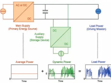
Fig. 1. Energy management strategy.
GA. Then, the interest of a systemic approach combining clus-tering analysis and synthesis of representative driving cycles is shown in Section V, which investigates the design of hybrid locomotives for shunting and switching operations in nonelec-trified areas. Finally, conclusions are drawn in Section VI.
II. DESIGNINDICATORSRELATED TODRIVINGCYCLES INHYBRIDARCHITECTURES
Here, we introduce different design indicators correlated with the sizing or efficiency of hybrid architectures, which are directly related to the driving cycles. In the following, these indicators will be used to classify and simplify driving cycles in the context of integrated design approaches aiming at optimizing architectures, sizing, and energy management [21].
A. First Set of Indicators Related to the System Sizing
The first three indicators (Pmax, Pav, and Eu) are relative
to the energy issue and are linked to the propulsion system sizing. Indeed, the design of power sources in hybrid archi-tectures strongly depends on the way that sources cooperate to fulfill the driving cycles. In these systems, a possible energy management consists in providing the average part of the load power by a primary energy source [22], [23] (see Fig. 1). The remaining power (i.e., the fluctuant part) is devoted to a storage system (i.e., the auxiliary source). With this particular power dispatching, the sizing of the main supply essentially depends on the average load powerPavdefined as
Pav= 1 ∆T ∆T Z 0 Pload(t) dt (1)
where∆T denotes the driving cycle duration, and Pload
repre-sents the load power required by the driving cycle. Furthermore, the sizing of the storage device can be characterized in terms of power, according to the maximal power imposed to this auxiliary supply, i.e.,Pmax− Pav, wherePmaxrepresents the
maximal load power related to the driving cycle. It also depends on the maximum energy quantityEutransferred to the storage
device. This energy can be computed as Eu= max
t∈[0, ∆T ](Es(t)) − mint∈[0, ∆T ](Es(t)) (2)
Fig. 2. Illustration of the storage cyclability estimation. (a) Cycle-to-failure characteristic. (b) Number of cycle calculation versus DOD levels.
where storage energy levelEsis defined as follows:
Es(t) = − t
Z
0
(Pload(τ ) − Pav) dτ. (3)
It should be noted thatEs(t) is a saturated integral with zero
as the upper limit so that the storage is only sized in discharge mode to avoid its oversizing during wide charge phases.
B. Second Set of Indicators Related to the System Performance
The first indicator of this second set is the cumulative distri-bution function (cdf), which is associated with the load power required by the driving profile. This function is defined on the space of the load power distribution and represents the system probability to operate at a power level less than or equal to a load power value.
Finally, the last indicator considered in this paper is related to the cyclability of the storage system. This indicator is essential in HEV design since it provides information on the storage lifetime. Therefore, we consider in this paper the total number of cycles Nc_tot imposed to the storage during the driving
cycle. This indicator is related to the storage state of charge (SOC) evolution and to the number of cycles to failurecF [24],
[25] defined as a function of the depth of discharge (DOD), which is specified in percentage [see Fig. 2(a)]. Considering the number of cycles to failure for DOD= 100% as a reference, we can express a “cycle weight”ωcyclefor lower DODs as [26]
ωcycle(DOD) =cF(100%)
cF(DOD)
. (4)
This weight evaluates the effect of a cycle at a given DOD with regard to a cycle at full DOD. Since the storage SOC evolution during a driving cycle consists in various cycles with different DODs, the total number of cyclesNc_totis computed
as follows: Nc_tot=
X
DODωcycle(DOD) × Ncycle(DOD) (5)
whereNcycle(DOD) denotes the number of cycles at a
particu-lar DOD. In practice, the DOD range is divided into equidistant intervals (typically, ten intervals), and the number of cycles in each interval is determined with the rainflow counting method [27], leading to a discretization of (3). This process is shown in Fig. 2(b). We point out that theNc_totindicator depends on
This highlights a coupling between the system features (i.e., the type of storage) and the system environment (here, the driving cycle).
In the following, we will consider as storage device the Hoppecke FNC1502HRNiCd battery cells [28] used in nominal conditions (i.e., temperature between 30◦C–40◦C, which are charged atC5and discharged at 2C5). In that case, the
cycle-to-failure curve plotted in Fig. 2(a) can be approximated as cF(DOD) = 966 × DOD−2.37 (6)
III. CLUSTERINGANALYSIS OFDRIVINGCYCLES
From the system point of view, the classification of driving cycles according to pertinent indicators with regard to design criteria and constraints is a part of a set of decision-making tools and constitutes a ridge phase, which is essential to the design process. Indeed, it must enable designers to evaluate the interest in a device that is specifically optimized for a given class, relative to the driving cycles, and this is compared with a device capable of simultaneously satisfying a set of classes. In other words, taking the well-known example of the car, “what do we gain by classifying and segmenting a vehicle range (urban, road, off-road, etc.) from the point of view of the cost/ performance ratio and with regard to usage and its occur-rences?” Classifying or segmenting may thus enable a notable improvement in certain criteria, such as the energy efficiency of the system. This is, for example, the case when, regarding a classification according to energy indicators, the segments or classes obtained are different from the commercial segmenta-tion or usage of the system.
In [29], a niching GA has been developed for the classifi-cation of driving cycles. This algorithm is based on the use of restricted tournament selection (RTS) [30] and a self-adaptive recombination technique [31], with the objective of maximizing the silhouette index [32] of the driving cycle data sets. In the following, we present an application of this algorithm to bench-mark railway profile (railway driving cycle) classifications.
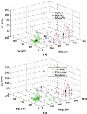
This benchmark, consisting of a set of 105 railway power profiles, is used to show the interest of clustering analysis in the context of hybrid system design. This set is composed of three subsets of profiles devoted to three different French railway systems: the BB 63000 old freight locomotive, the BB 460000 fret service locomotive, and the auxiliary supply for TGV (i.e., the French high-speed train). These systems have been considered to put forward the interest of the classification approach based on purely energy indicators. All profiles, which are represented by the load power demand as a function of time, are characterized according to the triplet of energy-based design indicators (Pav, Pmax, and Eu) aforementioned. The energy
management strategy is described in Fig. 1. All profiles are rep-resented versus the design indicators in Fig. 3(a). The centroid of each subset is also indicated with a black mark. In Fig. 3(b), the classification of the profiles obtained from the RTS runs after 500 generations is plotted. It is shown that the niching GA is capable of finding the correct partitioning of data by identifying three distinct clusters. The difference between both partitioning is only of 12% (i.e., 13 profiles over 105). Note that
Fig. 3. Profile classification of three railway systems. (a) Initial distribution of profiles. (b) Classification result.
the set of 105 profiles based on three different subsets of appli-cation (BB 63000, BB 460000, and TGV Aux) may present some similarities in terms of power/energy design indicators so that clustering profiles issued from different subsets may be energetically coherent. Thus, obtaining some differences between reference and RTS-based clustering is not necessary due to the niching GA convergence. All data are globally well classified, except elements located in the region covered by the three subsets. In this particular region of low power and energy, all profiles can be performed by the three hybrid supplies. Therefore, the assignment by the RTS of elements to the closest and most densely populated cluster (i.e., the cluster corresponding to TGV Aux driving profiles) is not surprising. This also explains the greater deviation of the cluster centroid relative to BB63 000 data. This cluster is more sensitive to par-titioning errors because of its small size. Moreover, both other cluster centroid positions are relatively unchanged by the RTS partitioning due to their larger size. These results also show the relevance of the proposed triplet for clustering analysis in the context of hybrid supply design.
IV. SYNTHESISPROCESS OFREDUCED AND
REPRESENTATIVEREAL-WORLDDRIVINGCYCLES
A. Principle
Beyond the classification methodology of the driving cycles presented in Section III, the next issue is to know how to best integrate the set of profiles from one class into a systemic design approach. In other words, we are looking to represent the information content of one set of profiles using a single
Fig. 4. Principle of the profile generation. (a) Profile generated by segment. (b) Pattern parameters.
and more compact, but representatively fictitious profile, to minimize computation costs within a system design process, particularly in the context of integrated design by optimization [21]. The fictitious profile is obtained by aggregating elemen-tary segments, as shown in Fig. 4. Each segment is character-ized by its amplitude∆Sn(∆Smin≤ ∆Sn≤ ∆Smax) and its
duration∆tn (0 ≤ ∆tn≤ ∆tcompact). Finding a compact
fic-titious profile consists in finding all segment parameters so that the generated profile fulfills all target indicators on the reduced duration∆tcompact. This results in solving an inverse problem
with 2N parameters, where N denotes the number of segments in the compact profile. This can be done using evolutionary al-gorithms and, particularly, with the clearing method [33], which is well suited to treat this kind of problem with high dimen-sionality and high multimodality. It should be also noted that the numberN of segments is optimized through a self-adaptive procedure [34]. The profile synthesis by an optimization cess is given in Fig. 5. The first stage consists of building pro-fileS(t) from the chromosome generated by the evolutionary algorithm, using the concatenation ofN elementary segments. A time-scaling step is performed after the profile genera-tion to fulfill the constraint related to the time duragenera-tion, i.e., Σ∆tn= ∆tcompact. The duration ∆tcompact of the obtained
cycle is considered to be a problem input. Although we are taking care to ensure that the synthesized profile is as com-pact as possible, the choice of its duration must check cer-tain constraints relative to the design indicators, as defined in Section II. In the following stage, we compute the profile indi-catorsIj(obtained from the synthesized profile), which are then
compared with the reference indicators Ijref (obtained from
the reference set of profiles). It enables error function ε (the function to be minimized using the evolutionary algorithm), which is expressed as ε =X j µ Ij− Ijref Ijref ¶2 (7) to be evaluated. This function is defined as the sum of quadratic scaled errors between reference and synthesized profile indicators.
B. Application on Railway Driving Cycles
Here, we study an example of ten railway driving cycles (see the Appendix) with the same duration (i.e., 4 h) used for the hybridization of the Diesel locomotive BB 63000. The architecture and the energy management strategy are in
Fig. 5. Synthesis process of representative profiles.
compliance with Fig. 1. The main supply is a Diesel engine, and the auxiliary supply is composed of Ni–Cd accumulator batteries (see Section V). The different driving cycles presented in the Appendix were assumed to be applied to the locomotive with the same occurrence. Moreover, batteries are supposed to be recharged after each 4-h driving cycle. Consequently, the reference indicators are chosen as follows.
– The average reference powerPav ref is set at the average
concatenation value for all cycles. We remind the reader that this power value corresponds to the Diesel engine sizing, which is a device for which consumption and “pollution” are optimum when this latter operates at its nominal power [23], [26].
– Pmax ref and Euref indicators are set at the more
constraining values for all of the ten driving cycles, i.e., Pmax ref= max Pmax(i) and Euref= max Eu(i),
wherei denotes the driving cycle index (i = 1, . . . , 10). This enables us to guarantee that the system being de-signed will satisfy all driving cycles.
– The performance and lifetime indicators are considered to be average. The choice of useful reference energy Euref enables the storage size to be determined, and as
a consequence, we are able to estimate the number of cycles consumed for each driving cycles. The number of reference cyclesNc_tot ref is thus determined by the
average value of the cycle number per hour across all profiles. For statistical reference indicator Istat ref, we
consider the cdf associated with the concatenation of all cycles.
Note that the nature of the design indicators imposes sub-stantial minimum times. This refers most particularly to the useful energy indicator or the number of cycles that are closely coupled with the profile duration. The representative railway driving profile is obtained through the concatenation of 148 segments (see Fig. 6). We give in Table I the values of sizing and performance indicators of this profile in comparison with the reference values. Note that the statistic errorεstatis defined
as the mean square error, which is computed over 100 equally spaced points, between both cdfs relative to the power of the driving cycles, i.e.,
εstat= 1 100× 100 X i=1
µ cdf(i) − cdfref(i)
cdf(i)
¶2
Fig. 6. Result of the compact profile synthesis process on ten driving cycles. (a) Representative driving profile. (b) Distribution functions.
TABLE I
CHARACTERIZATIONINDICATORS OF THEREPRESENTATIVEPROFILE
The results show that our signal synthesis approach performs well and is capable of finding a profile shape representing the whole set of driving cycles. It should be noted that the “fictitious” profile duration is about 14.5 h. In comparison with the global duration of the ten profiles (i.e., 40 h), the profile duration has been reduced by 2.8. Consequently, in a design optimization process such as in [35], the simulation of any hybrid electric system will also be reduced.
V. INTEGRATEDOPTIMALDESIGN OF AHYBRID
LOCOMOTIVEFROMREAL-WORLDDRIVINGCYCLES
Here, we are proposing to show the complete process for a systemic design approach. Starting with the classification of real profiles (see Section III), the profile synthesis process (see Section IV) based on a set of railway driving cycles is used to complete the integrated design by optimization of the railway hybrid system. The idea is to design a hybrid locomotive optimized for each profile class and to compare the cost of annual ownership of the devices obtained, with the design of a single locomotive capable of satisfying all profile classes at once. This general approach to system design is founded on a reference database corresponding to an example using ten railway driving cycles with iso-times (4 h per profile). We assume that the storage SOC of Ni–Cd batteries is reset to 100% after each 4-h cycle sequence. In Fig. 7, we show the various stages of the proposed comparative study.
A. Hybrid Locomotive Model
1) Power Flow Model: The power flow model determines the energetic characteristics of the locomotive power sources i.e., powerP , energy E, and the SOC for the storage elements. Considering a given power profilePM, an energy management
controller provides power reference values for the Diesel en-gine(PDEref) and the batteries (PBTref). These references are
Fig. 7. General system approach, from classification to optimal design.
Fig. 8. Power flow model of the Diesel engine.
obtained according to the management strategy of Fig. 1. The power flow model of the Diesel engine is given in Fig. 8. It allows us to obtain power referencePDErefand a start/stop
con-trol, the Diesel engine powerPDE, the corresponding energy
EDE, the quantity of fuel consumedQfuel, and the
correspond-ing quantity of emitted carbon dioxideQCO2. The parameters
of this model are the converter efficiency associated with the Diesel engine (typically,ηDE= 96%), the Diesel power limit
PDE max, and the specific fuel consumption (SFC)
character-istic. This characteristic has been extrapolated with a fifth-order polynomial as a function of the Diesel engine power as follows [26]: SFC(PDE) = SFCN 5 X i=1 bi µ PDE PDEN ¶ (9)
where the polynomial coefficients areb0= 1.94, b1= −6.44,
b2= 18.57, b3= −27.22, b4= 19.72, and b5= 1.94. PDEN
denotes the nominal power of the Diesel engine, and SFCN
represents the SFC at this power estimated at 202.45 g/kW. The previous relation has been validated for three Diesel en-gines of the Fiat Powertrain Technologies Group [36], i.e., the N67 TM2A with 125 kW, the C78 TE2ES with 236 kW, and the C13 TE2S with 335 kW. It should be noted that the SFC is at the minimum when the Diesel engine operates at its nominal power PDEN. Therefore, the energy management
Fig. 9. Battery power flow model.
Fig. 10. Battery cell electric model.
close to this power. Note also that the maximal Diesel engine power is considered 10% higher than the nominal power. The quantity of CO2 emitted (in kilograms per liter) is directly
proportional to the fuel quantity consumed and is estimated as follows [37]:
QCO2 = 2.66 × Qfuel. (10)
The battery power flow model is given in Fig. 9. In this model, the storage powerPBT, the corresponding energyEBT, and the
associated SOCSOCBTare computed from the initial energetic
capacityEBT0, the reference power resulting from the energy
management controller PBT0, the maximum discharge power
Pdchmaxand the maximum charge powerPchmaxof the battery
pack, and the efficiency ηBT. Note that the total energetic
capacity of a pack depends on the total number of cells and on the capacity of each cell.
2) Electric Model: Beyond the power flow model, which only specifies power and energy transfers, one further step is achieved at the electric model level, which provides voltages and currents. AnRC electric model is used to obtain the electri-cal variables (current and voltage) in a battery cell (see Fig. 10). Technological data values corresponding to Hoppecke FNC1502HR battery cells of 135-Ah capacity(C5= 135 Ah)
are considered in these models [28]. The battery resistance rBT and its electromotive forceeBT are interpolated from the
manufacturer data as a function of the cell SOCq, i.e., ½ rBT= 2.83 − 12.88q + 24.88q2− 20.83q3+ 6.28q4
eBT= 0.99 + 1.06q − 1.82q2+ 1.11q3. (11)
As shown in Fig. 10, the current and voltage in the cell are computed from the cell powerpBT. This power can be obtained
from the global power of the pack PBT. resulting from the
power flow model, i.e.,
pBT= PBT/(NPBT× NSBT) (12)
where NSBT and NPBT denote the number of battery cells
in series and the associated number of branches in parallel, respectively.
3) Geometric Model: From the data provided by manufac-turers, the volume in square meters of the Diesel engine can be expressed in terms of its nominal powerPDEN in Watts using
the following relation:
ΩDE= 3 × 10⁻⁵PDEN+ 0.09. (13)
The battery volume, taking into account the cooling systems and associated electronic modules (such as charge state balanc-ing and thermal control), is given by the followbalanc-ing:
ΩBT= λBT× NPBT× NSBT× ΩBT0 (14)
whereΩBT0= 4.33 × 10⁻³m3, andλBT= 1.8 represents the
assembly coefficient, which considers intercellular spaces, elec-tronic modules, and cooling systems.
4) Battery Lifetime Model: The battery lifetime LFTBT is
directly related to the number of battery cycles consumed during the railway profile. It is expressed by the product of the cycle number consumed by each cellNc_totand the number of
cells in series NSBTand in parallel NPBT, i.e.,
LFTBT= NPBT× NSBT× Nc_tot. (15) 5) Cost Model: Similar to the geometric model, the cost model uses empiric relations derived from manufacturer data to evaluate the cost of each energetic source embedded in the locomotive. The global cost in euros of the Diesel engine CDE, including its installation, can be interpolated by a linear
function versus the nominal power, i.e.,
CDE[k C] = 0.28 × PDEN+ 14.5. (16)
To take account of the Diesel engine costs during the loco-motive exploitation (including repairs and maintenance), the previous relation has been modified. It has been estimated by the French National Railways Company (SNCF) that the Diesel engine cost over ten years is in, average, three times higher than the purchase cost [35]. Therefore, the previous relation can be modified as follows:
CDE[k C/yr] =
3
10(0.28 × PDEN+ 14.5). (17) The cost of the battery cells is calculated from the cycle cost, which allows taking account of purchase costs (including installation costs) and maintenance costs (directly related to the battery lifetime). A battery deep cycle (100% of DOD) cost has been estimated to 0.122 C. By considering the LFTBT
stress estimator that evaluates the total number of cycles for the battery pack on a particular railway profile, the battery cost per yearCBTcan be expressed as
CBT[k C/yr] = 0.122 × 10⁻³× LFTBT×
∆τyr
∆τ (18)
where∆τyrrepresents the locomotive exploitation in one year
TABLE II
HYBRIDLOCOMOTIVEDESIGNVARIABLES
duration. Finally, with a Diesel fuel cost of about 1.35C/l, the global cost per year can be estimated as
Cfuel[k C/yr] = 1.35 × 10⁻³× Qfuel×
∆τyr
∆τ . (19)
B. Optimization Process
1) Optimization Parameters: The design variables and their associated bound are shown in Table II.
2) Optimization Constraints: Four inequality constraints that are classically formulated in terms of minimization (i.e., gi≤ 0) have to be fulfilled to ensure the locomotive feasibility.
These constraints can be separated into two groups. The first three constraints (g1,g2, andg3) do not require the locomotive
simulation on its driving cycle and are qualified as
presimu-latingconstraint. On the contrary, the last constraint(g4) is a postsimulatingconstraint, which can be only evaluated from the driving cycle simulation. With the aim of improving the CPU time related to the optimization step, this constraint is computed only if all presimulating constraints are fulfilled. Otherwise, it receives the maximum penalty (i.e.,g4→ ∞).
– The first constraintg1verifies that the volume available
for energy sources is lower than 32 m3, i.e.,
g1= ΩBT+ ΩDE− 32 ≤ 0 (20)
without considering at this stage the static converter volume associated with battery blocks.
– The second constraintg2is related to the minimum
num-ber of battery cellsNBT minrequired to fulfill the driving
cycle. This number can be determined from a battery sizing procedure based on the power flow model accord-ing to [23]. Finally, the constraintg2is expressed as
g2= NBT min− NPBT× NSBT≤ 0. (21)
– Taking into account the elevated structure of choppers (from batteries toward bus) and of the maximum cyclic ratio αmax, the maximum voltage of a battery block
VBT max must be then less than αmax× Vbus. If the
maximum voltage of a battery element is known, the constraintg3is written as follows:
g3= NSBTVBT max− αmax× Vbus≤ 0. (22)
– If all previous constraints are satisfied, the locomotive sizing can be refined by evaluating the static converter volumeΩCBT associated with battery blocks. This
vol-ume can be computed from the driving cycle simulation by determining the maximum current in each battery block and, consequently, the filtering inductance required
Fig. 11. Classification of railway profiles according to sizing indicators.
to limit the current ripples (see [35]). Finally, constraint g4can be expressed as
g4= ΩBT+ ΩDE+ ΩCBT− 32 ≤ 0. (23) 3) Optimization Criteria: The hybridization approach aims at minimizing the investment and usage costs and the environ-mental cost (tonnes of CO2). This systemic evaluation has been
done with respect to a full Diesel locomotive of the same power. As the quantity of CO2released is proportional to the quantity
of fuel burn [see (10)], the environmental cost optimization can be therefore reflected in the optimization of the quantity of fuel burn. This enables us to reduce the multiobjective optimization problem into a single optimization problem consisting in the minimization of the annual total cost of ownership (TCO), integrating at the same time the costs of investment and usage (maintenance, lifetime, and fuel burn) as follows:
TCO= CDE+ CBT+ Cfuel. (24)
C. Railway Profile Classification
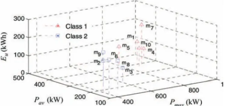
We move now to the classification of the railway driving cycles given in the Appendix according to the design indicators {Pmax, Pav, Eu}. The result obtained by applying the
RTS-based classification algorithm presented in Section III is shown in Fig. 11. It is shown that two different classes are obtained, each containing five elements.
D. Synthesis of Representative Railway Profiles
In this second study phase, we have applied the represen-tative and compact profile synthesis process for each class C1 and C2, and for CΣ= (C1∪ C2), which is composed of
the global set of profile. The reference indicators that enable the characterization of the representative profile are chosen as indicated in Section IV-B.
1) ClassC1Representative Profile:M1rep: We set the
dura-tion of the representative profile for classC1at 4 h, which
corre-sponds to save a 1/5 ratio over the total duration of concatenated profiles (20 h). The result of the synthesis process is given in Fig. 12(a). This representative profileM1repis obtained through
the concatenation of 125 segments and perfectly fulfills the reference indicators [see Table III and Fig. 12(b)].
2) Class C2 Representative Profile: M2rep: The duration
Fig. 12. Result of the compact profile synthesis process for class C1.
(a) Representative profile M1rep. (b) Distribution functions.
TABLE III
CHARACTERIZATIONINDICATORS OF THE
REPRESENTATIVEPROFILEM1rep
Fig. 13. Result of the compact profile synthesis process for class C2.
(a) Representative profile M2rep. (b) Distribution functions.
TABLE IV
CHARACTERIZATIONINDICATORS OF THE
REPRESENTATIVEPROFILEM2rep
corresponds to save a ratio of 1/3.3 over the total duration of concatenated profiles (20 h). The result of synthesis is given in Fig. 13(a). This representative profileM2repis obtained through
the concatenation of 126 segments and perfectly fulfills the reference indicators [see Table IV and Fig. 13(b)].
3) ClassCΣRepresentative Profile:MΣrep: The
represen-tative and compact profile related to the set of ten driving cycles corresponds with the results presented in Section IV (see Fig. 6 and Table I).
E. Integrated Design by Optimization
Having determined the representative profiles, we proceed here to the integrated design of three hybrid locomotives that
TABLE V
RESULTS OFDESIGN BYOPTIMIZATION INHYBRIDLOCOMOTIVES
are optimized per profile class. Let L1rep, L2rep, andLΣrep
denote the hybrid locomotives, which are sized for classesC1,
C2, andCΣ, respectively, from representative railway profiles
M1rep,M2rep, andMΣrep. To validate the consistency of the
design results and to emphasize the synthesis process efficiency in terms of computation time, we have also sized three hybrid locomotives, which are optimized from a real profile class. In these cases, locomotives are designed in a “classical way” by considering the concatenation of all of the five driving cycles (instead of the corresponding compact and representative profile) under the hypothesis that the battery SOC is set to its initial value after each 4-h cycle. Thus, we also denote the hybrid locomotives sized for each classC1,C2, andCΣfrom
real complete cycles M1real, M2real, and MΣreal, by L1real,
L2real, and LΣreal, respectively. Under the hypothesis that all
initial profiles are realized with the same occurrence over a year with 8 h of use per day (two successive cycles per day) for each locomotive, the design results are given in Table V. The optimization algorithm used at the heart of the integrated design process is based on a GA and is coupled to the different hybrid locomotive models presented earlier.
The design results obtained for each profile class proves the effectiveness of the representative profile synthesis process in the system design approach. Indeed, we obtain practically nearly the same sizing from the hybrid locomotive by consider-ing, on one hand, the fictitious representative profile, and, on the other hand, the concatenation of real profiles in the envisaged class. It should also be noted that the annual performance criteria (TCO and CO2emissions) estimated on the set of real
profiles are equivalent. Finally, we mention in Table V the computational timeTcrequired for the locomotive optimization
in all investigated cases. It should be noted that all results were obtained from a GA run after 1000 generations using a population size of 100 individuals. Thus,Tc is relative to the
CPU time needed for those runs according to the driving profile used in the optimization process (i.e., the set of real driving cycles or the compact representative profile). We observe in Table V a significant saving in terms of CPU time between the two approaches. The synthesized representative profiles enable a computation saving, which is increased to 4.5 days for class C1, 4.1 days for classC2, and 6.6 days for classCΣ.
F. Design Result Comparison
Based on 8 h/day of use for each locomotive, the ten initial classCΣ profiles, with a total length of 40 h, are repeated 73
times over the course of one year, whereas the five profiles in classC1 of the same length are each repeated 146 times each
year. To evaluate the interest in the classification (or segmenta-tion), we compare the average annual costs of the two locomo-tivesL1andL2with that of locomotiveLΣby considering the
designs obtained with the representative and compact driving profiles. The average annual TCO ofL1andL2is estimated at
TCO(L1 & L2) = 0.5 × (TCO(L1(C1) + TCO(L2(C2)) ≈
300 kC/yr compared with TCO(LΣ) ≈ 320 kC/yr,
repre-senting the annual TCO of a single locomotiveLΣ
perform-ing all drivperform-ing cycles. We observe that, for this ten-profile example, the design of two locomotives optimized per profile class enables a saving of 20 kC/yr (∼6%) compared with a single locomotive capable of satisfying all profiles on the list of specifications. Conversely, although it is less profitable finan-cially, the single locomotive is better in terms of environment. Indeed, the annual use of this locomotive generates around 460 tonnes of CO2 versus 504 T of CO2 (∼ +9%) emitted
during an average annual exploitation of both locomotivesL1
andL2. The choice of whether to design a single locomotive
or two different locomotives L1 and L2 is governed by a
compromise between financial and ecological aspects. Beyond the result of this particular application, the interest of the complete approach (classification–profile synthesis–integrated optimal design) proposed in this paper is to facilitate the choice of design users, i.e., SNCF, in terms of segmentation of the product range and then sizing. These choices can be directly put forward into perspective with regard to the essential design criteria (i.e., ownership and climate costs).
VI. CONCLUSION
In this paper, a systemic approach integrating driving cycles has been proposed for the design of hybrid autonomous loco-motives. Efforts spent to achieve this process emphasize the prime importance of mission profile issues in HEVs and, more generally, of environmental variables for any class of systems.
This approach particularly exploits clustering analysis with the aim of identifying driving cycle classes that is relevant for market segmentation. Those classes are found using specific design indicators related to the driving cycle features and the propulsion hybrid system performance. Then, a synthesis procedure is applied to determine compact and representative profiles related to a given class or to a set of classes. Using the resulting profiles in the design process instead of the set of real driving cycles allows significant savings in computational time. It has been clearly shown through the application of the proposed design approach on the optimization of a hybrid autonomous locomotive devoted to shunting and switching operations. In addition, our approach also forms, for designer users, an “aid to market segmentation associated with an aid to system design.” It can be extended to other kinds of systems without much difficulty, including standalone renewable energy systems and similar stochastic environmental variables (e.g., wind speed profiles).
APPENDIX
SET OFTENDRIVINGCYCLES OF AHYBRID
AUTONOMOUSLOCOMOTIVEDEVOTED TOSHUNTING ANDSWITCHINGOPERATIONS
REFERENCES
[1] Emission Test Cycles for the Certification of Light Duty Vehicles in
Eu-rope, EEC Directive 90/C81/012009.
[2] H. Fan, G. E. Dawson, and T. R. Eastham, “Model of electric induction motor drive system,” in Proc. IEEE Can. Conf. Elect. Comput. Eng., Sep. 14–17, 1993, vol. 2, pp. 1045–1048.
[3] A. Kleimaier and D. Schröder, “Optimization strategy for design and control of a hybrid vehicle,” in Proc. 6th Int. Workshop Adv. Motion
Control, Nagoya, Japan, 2000, pp. 459–464.
[4] S. Barsali, C. Miulli, and A. Possenti, “A control strategy to minimize fuel consumption of series hybrid electric vehicles,” IEEE Trans. Energy
Convers., vol. 19, no. 1, pp. 187–195, Mar. 2004.
[5] Emission Standards for Locomotives and Locomotive Engines; Final
Rule, U.S. Environmental Protection Agency (EPA), 63 Federal Register 18978, 1998.
[6] S. Zorrofi, S. Filizadeh, and P. Zanetel, “A simulation study of the impact of driving patterns and driver behavior on fuel economy of hybrid transit buses,” in Proc. IEEE Veh. Power Propulsion Conf., Dearborn, MI, USA, 2009, pp. 572–577.
[7] B. A. Holmen and D. A. Niemeier, “Characterizing the effects of driver variability on real-world vehicle emissions,” Transp. Res. Part D, vol. 3, no. 2, pp. 117–128, Mar. 1998.
[8] P. De Haan and M. Keller, “Real-world driving cycles for emission mea-surements: ARTEMIS and Swiss cycles,” INFRAS, Zurich, Switzerland, BUWAL SRU Nr.255: Bern, 2001.
[9] W. T. Hung, H. Y. Tong, C. P. Lee, K. Ha, and L. Y. Pao, “Development of practical driving cycle construction methodology: A case study in Hong-Kong,” Transp. Res. Part D, Transp. Environ., vol. 12, no. 2, pp. 115–128, Mar. 2007.
[10] E. Tara, S. Shahidinejad, S. Filizadeh, and E. Bibeau, “Battery storage sizing in a retrofitted plug-in hybrid electric vehicle,” IEEE Trans. Veh.
Technol., vol. 59, no. 6, pp. 2786–2794, 2010.
[11] M. André, “The ARTEMIS European driving cycles for measuring car pollutant emissions,” Sci. Total Environ., vol. 334/335, pp. 73–84, Dec. 2004.
[12] M. Andre, R. Joumard, R. Vidon, P. Tassel, and P. Perret, “Real-world European driving cycles, for measuring pollutant emissions from high-and low-powered cars,” Atmosp. Environ., vol. 40, no. 31, pp. 5944–5953, Oct. 2006.
[13] Q. Shi, D. Qiu, N. Wang, and R. Wang, “The impact analysis of the accuracy of driving cycle based on division of running statuses,” in Proc.
ICEICE, Wuhan, China, 2011, pp. 2767–2772.
[14] V. Schwarzer, R. Ghorbani, and R. Rocheleau, “Drive cycle generation for stochastic optimization of energy management controller for hybrid vehicles,” in Proc. IEEE Int. Conf. Control Appl., Part IEEE Multi-Conf.
Syst. Control, Yokohama, Japan, 2010, pp. 536–540.
[15] I. Kolmanovsky, I. Siverguina, and B. Lygoe, “Optimization of powertrain operating policy for feasability assessment and calibration: Stochastic dynamic programming approach,” in Proc. IEEE Amer. Control Conf., Anchorage, AK, USA, 2002, vol. 2, pp. 1425–1430.
[16] P. Jiang, Q. Shi, W. Chen, Y. Li, and Q. Li, “Investigation of a new con-struction method of vehicle driving cycle,” in Proc. 2nd ICITA, Changsha, China, 2009, pp. 210–214.
[17] C. C. Lin, H. Peng, and J. W. Grizzle, “A stochastic control strategy for hybrid electric vehicles,” in Proc3 IEEE Amer. Control Conf., Boston, MA, USA, 2004, vol. 5, pp. 4710–4715.
[18] G. Ripaccioli, D. Bernardini, S. Di Cairano, A. Bemporad, and I. V. Kolmanovsky, “A stochastic model predictive control approach for series hybrid electric vehicle power management,” in Proc. ACC, Balti-more, MD, USA, 2010, pp. 5844–5849.
[19] T. K. Lee and Z. S. Philipi, “Synthesis and validation of representative real-world driving cycles for plug-in hybrid vehicles,” in Proc. IEEE Veh.
Power Propulsion Conf., Lille, France, 2010, pp. 1–6.
[20] G. Souffran, L. Miegevielle, and P. Guérin, “Simulation of real-world vehicle missions using a stochastic Markov model for optimal design purposes,” in Proc. IEEE VPPC, Chicago, IL, USA, Sep. 6–9, 2011, pp. 1–6.
[21] X. Roboam, Ed., Integrated Design by Optimization of Electrical Energy
Systems (ISTE). Hoboken, NJ, USA: Wiley, 2012.
[22] M. Ehsani, Y. Gao, and K. Butler, “Application of electrically peaking hy-brid (ELPH) propulsion system to a full-size passenger car with simulated design verification,” IEEE Trans. Veh. Technol., vol. 48, no. 6, pp. 1779– 1787, Nov. 1999.
[23] C. R. Akli, X. Roboam, B. Sareni, and A. Jeunesse, “Energy management and sizing of a hybrid locomotive,” in Proc. 12th EPE, 2007, pp. 1–10. [24] S. Drouilhet and B. L. Johnson, “A battery life prediction method for the
hybrid power applications,” in Proc. 35th AIAA Aerosp. Sci. Meet. Exhib., 1997, pp. 1–14.
[25] R. Dufo-Lopez and J. L. Bernal-Agustin, “Multi-objective design of PV-wind-diesel-hydrogen-battery systems,” Renew. Energy, vol. 33, no. 12, pp. 2559–2572, Dec. 2008.
[26] A. Jaafar, C. R. Akli, B. Sareni, X. Roboam, and A. Jeunesse, “Sizing and energy management of a hybrid locomotive based on flywheel and accumulators,” IEEE Trans. Veh. Technol., vol. 58, no. 8, pp. 3947–3958, Oct. 2009.
[27] S. H. Baek, S. S. Cho, and W. S. Joo, “Fatigue life prediction based on the rainflow cycle counting method for the end beam of a freight car bogie,”
Int. J. Automotive Technol., vol. 9, no. 1, pp. 95–101, Feb. 2008.
[28] [Online]. Available: http://www.hoppecke.com, 2012.
[29] A. Jaafar, B. Sareni, and X. Roboam, “Clustering analysis of railway driving missions with niching,” Int. J. Comput. Math. Elect. Electron.
Eng. (COMPEL), vol. 31, no. 3, pp. 920–931, 2012.
[30] G. Harik, “Finding multimodal solutions using restricted tournament se-lection,” in Proc. 6th Int. Conf. Genetic Algorithms, 1995, pp. 24–31. [31] B. Sareni, J. Régnier, and X. Roboam, “Recombination and
self-adaptation in multi-objective genetic algorithms,” in Proc. Artif.
Evolu-tion, vol. 2936, Lecture Notes in Computer Science, 2004, pp. 115–126. [32] P. J. Rousseeuw, “Silhouettes: A graphical aid to the interpretation and
validation of cluster analysis,” Comput. Appl. Math., vol. 20, pp. 53–65, Nov. 1987.
[33] A. Petrowski, “A clearing procedure as a niching method for genetic algorithms,” in Proc. IEEE Int. Conf. Evolutionary Computation, Nagoya, Japan, 1996, pp. 798–803.
[34] A. Jaafar, B. Sareni, and X. Roboam, “Signal synthesis by means of evolutionary algorithms,” Inverse Probl. Sci. Eng., vol. 20, no. 12, pp. 93– 104, Jan. 2012.
[35] C. R. Akli, X. Roboam, B. Sareni, and A. Jeunesse, “Integrated optimal design of a hybrid locomotive with multiobjective genetic algorithms,”
Int. J. Appl. Electromagn. Mech., vol. 4, no. 3/4, pp. 151–162, 2009. [36] [Online]. Available: http://www.fptindustrial.com, 2012
[37] L. A. Graham, “Greenhouse gas emissions from light duty vehicles under a variety of driving conditions,” in Proc. IEEE EIC Climate Change
Technol., 2006, pp. 1–8.
Amine Jaafar was born in Sousse, Tunisia, in 1983.
He received the Engineering degree in electrical engineering from Ecole Nationale d’Ingénieur de Monastir, Monastir, Tunisia, in 2007 and the Ph.D. degree from the University of Toulouse, Toulouse, France, in 2011. He is currently working as assistant professor with INP-ENSEEIHT, Toulouse, France, where he is studying fuel cell applications as a researcher with the Laboratory on Plasma and Con-version of Energy (LAPLACE).
Bruno Sareni was born in Bron, France, in 1972.
He received the Ph.D. degree from Ecole Centrale de Lyon, Écully, France, in 1999.
He is currently a Professor in electrical engineer-ing and control systems with the National Polytech-nic Institute of Toulouse, Toulouse, France. He is also a Researcher with the Laboratory on Plasma and Conversion of Energy (LAPLACE), University of Toulouse, Toulouse. His research interests include the analysis of complex heterogeneous power de-vices in electrical engineering and the optimization of these systems using artificial evolution algorithms.
Xavier Roboam received the Ph.D. degree in
elec-trical engineering from the University of Toulouse, Toulouse, France, in 1991.
Since 1992, he has been with the Laboratory on Plasma and Conversion of Energy, University of Toulouse, as a Full-Time Researcher. Since 1998, has been the Head of the Research Group in Electrical Energy and Systemics (GEnESys), whose objective is to process the design problem in electrical en-gineering at a “system level.” He has developed methodologies specifically oriented toward multi-field system design for applications such as electrical embedded systems or renewable energy systems.