This is an author-deposited version published in:
http://oatao.univ-toulouse.fr/
Eprints ID: 10903
To link to this article: DOI: 10.1115/1.4026311
URL:
http://dx.doi.org/10.1115/1.4026311
To cite this version:
François, Benjamin and Laban, Martin and Costes,
Michel and Dufour, Guillaume and Boussuge, Jean-François In-Plane
Forces Prediction and Analysis in High-Speed Conditions on a
Contra-Rotating Open Roto. (2014) Journal of Turbomachinery, vol. 136 (n° 8).
ISSN 0889-504X
O
pen
A
rchive
T
oulouse
A
rchive
O
uverte (
OATAO
)
OATAO is an open access repository that collects the work of Toulouse researchers and
makes it freely available over the web where possible.
Any correspondence concerning this service should be sent to the repository
administrator:
[email protected]
Benjamin Franc¸ois
Aerodynamic Department, Airbus Operations S.A.S., 306 Route de Bayonne, Toulouse Cedex 9 31000, France e-mail: [email protected]
Martin Laban
Flight Physics and Loads Department, National Aerospace Laboratory, NLR, Anthony Fokkerweg 2, Amsterdam 1059CM, Netherlands e-mail: [email protected]
Michel Costes
Onera, The French Aerospace Lab, 8 Rue des Vertugadins, Meudon F-92190, France e-mail: [email protected]
Guillaume Dufour
Institut Sup!erieur de l’A!eronautique et de l’Espace (ISAE), Universit!e de Toulouse, 10 avenue Edouard Belin, 31400 Toulouse, France e-mail: [email protected]
Jean-Franc¸ois Boussuge
CFD Department, CERFACS, 42 avenue Gaspard Coriolis, 31000 Toulouse, France e-mail: [email protected]
In-Plane Forces Prediction
and Analysis in High-Speed
Conditions on a Contra-Rotating
Open Rotor
Due to the growing interest from engine and aircraft manufacturers for contra-rotating open rotors (CROR), much effort is presently devoted to the development of reliable com-putational fluid dynamics (CFD) methodologies for the prediction of performance, aero-dynamic loads, and acoustics. Forces transverse to the rotation axis of the propellers, commonly called in-plane forces (or sometimes 1P forces), are a major concern for the structural sizing of the aircraft and for vibrations. In-plane forces impact strongly the sta-bility and the balancing of the aircraft and, consequently, the horizontal tail plane (HTP) and the vertical tail plane (VTP) sizing. Also, in-plane forces can initiate a flutter phe-nomenon on the blades or on the whole engine system. Finally, these forces are unsteady and may lead to vibrations on the whole aircraft, which may degrade the comfort of the passengers and lead to structural fatigue. These forces can be predicted by numerical methods and wind tunnel measurements. However, a reliable estimation of in-plane forces requires validated prediction approaches. To reach this objective, comparisons between several numerical methods and wind tunnel data campaigns are necessary. The primary objective of the paper is to provide a physical analysis of the aerodynamics of in-plane forces for a CROR in high speed at nonzero angle of attack using unsteady simulations. Confidence in the numerical results is built through a code-to-code comparison, which is a first step in the verification process of in-plane forces prediction. Thus, two computa-tional processes for unsteady Reynolds-averaged Navier–Stokes (URANS) simulations of an isolated open rotor at nonzero angle of attack are compared: computational strategy, open rotor meshing, aerodynamic results (rotor forces, blades thrust, and pressure distri-butions). In a second step, the paper focuses on the understanding of the key aerodynamic mechanisms behind the physics of in-plane forces. For the front rotor, two effects are pre-dominant: the first is due to the orientation of the freestream velocity, and the second is due to the distribution of the induced velocity. For the rear rotor, the freestream velocity effect is reduced but is still dominant. The swirl generated by the front rotor also plays a major role in the modulus and the direction of the in-plane force. Finally, aerodynamic interactions are found to have a minor effect
1
Introduction
In the context of increasing costs for fuel, the development of new aircraft designs is mainly driven by the need to reduce fuel burn. To reach this end, new engine concepts such as contra-rotating open rotors appear to be one suitable option for the single aisle segment, currently dominated by the Airbus A320 and Boe-ing 737. This concept was the focus of a large research effort led by NASA and US industry in the late 1970s and 1980s, motivated by the high fuel costs arising from the 1973 oil crisis [1]. Signifi-cant advances were achieved, but due to the decrease in oil prices, the interest in bringing those engines to market waned. Presently, the CROR concept appears again to be one promising option for powering the new generation of short-range aircraft.
This new concept raises major challenges for aircraft manufac-turers. One of them is the impact of forces transverse to the rota-tion axis of the propellers, commonly named in-plane forces1,
which are caused by a nonhomogeneous inflow velocity flow field in the propeller plane. Such conditions are encountered when the
far-field inflow has an angle of attack with respect to the rotation axis (incidence, sideslip) or for an installed propeller configura-tion. Therefore, it is essential to predict these forces for the struc-tural design of the installed engine system. In-plane forces contribute also to the sizing of HTP and VTP because these forces need to be counterbalanced to meet handling quality requirements. Then, in-plane forces can initiate a flutter phenomenon on the blades or on the whole engine system. Finally, these forces are unsteady and may lead to vibrations on the whole aircraft that may degrade the comfort of the passengers and lead to structural fatigue.
In order to predict accurately the in-plane forces on open rotors, a lot of effort is devoted to the development and the validation of methods and tools for high-fidelity aerodynamic simulations and to wind tunnel test campaigns on open rotor configurations. The work presented in this paper focuses on the assessment and the understanding of in-plane forces on an isolated open rotor config-uration at high-speed (conditions in which in-plane force magni-tude can reach the same order of the thrust level) at nonzero angle of attack.
Numerous works have been done in the past to predict and understand the origin of the in-plane forces around propellers. The in-plane forces on propellers at nonzero angle of attack were pointed out for the first time in 1909 by Lanchester [2]. A few years later, the first basic theories emerged with Harris [3] and Glauert [4] who proposed an analogy with a fin: A propeller at Contributed by the International Gas Turbine Institute (IGTI) of ASME for
publication in the JOURNAL OFTURBOMACHINERY. Manuscript received January 17,
2013; final manuscript received December 11, 2013; published online January 31, 2014. Assoc. Editor: Alok Sinha.
1The expression1P-forces (1P stands for once-per-revolution) can also be found
in literature to define the in-plane forces on a propeller. However, the 1P-forces expression will not be used in this work.
nonzero angle of attack develops a normal force in the orthogonal direction of the incoming velocity vector as a fin. Forces and moments arising were expressed with an analytical expression using the thrust and torque of an uninclined propeller. Forces applied on propellers were split into the forces along the rotation axis, commonly called thrust, and the force normal to the rotation axis. In 1935, Glauert [5] proposed a widely used analytical expression of the normal force. For an inclined propeller, this force is a function of the angle of inclination, the advance ratioJ, the power coefficient Cp, and the thrust distribution along the
blade. Glauert’s definition considered only the component con-tained in the vertical plane for an inclined propeller. Lateral force was not taken into account. Comparison of Glauert’s theory to ex-perimental results [6] showed little discrepancies, but this valida-tion was limited up to blade settings angles of 45 deg and advance ratio value of 2.0. Later, this theory was exploited by Ribner [7] who extended it to contra-rotating propellers. From the 1950s to the 1980s, fewer articles about propellers were published, prob-ably due to a decreasing interest in propellers and the emergence of the turbofan technology. These analytical models were rapid methods for the improvement of propellers aerodynamics but were not valid for compressible flows.
After the oil crisis, many studies on propellers reemerged in the 1980s with the first three-dimensional steady Euler computations at high speed with the work of Bober et al. [8]. The move to com-putational procedures for solving the fluid dynamic equations was motivated by two main reasons. First, analytical models were only valid at low-speed and, thus, unfit for transonic flows. Second, Euler computations were accurate means of determining the aero-dynamic characteristics of a complex blade for which the three-dimensional geometry cannot be handled by existing analytical models. The computations of Bober et al. were performed on iso-lated propellers at zero angle of attack. The computational domain was reduced to a single blade passage with periodicity boundary conditions. The flow was solved with a steady approach in the rotating frame. Comparison with experiments showed that the power coefficient is overpredicted, but the variation regarding its blade angle was well captured. According to Bober et al., these discrepancies could be attributed to the viscous effects. These methods were extended to contra-rotating propellers by Wong et al. [9] and Nicoud et al. [10]. The rotor-rotor interface was modeled with a mixing-plane condition [11]. First aerodynamic simulations of propellers at nonzero angle of attack at high-speed (Mach number from 0.6 to 0.8) were achieved by Nallasamy [12] in 1994. All the blades have to be accounted for in the computa-tion because there are no flow periodicity relacomputa-tions. The flow was solved with an unsteady approach because the inflow seen by the blade varies depending on its azimuthal position. Pressure trans-ducers measurements over a rotation for different radii were com-pared to the numerical simulation results and showed acceptable discrepancies. Nonetheless, nonlinear variations of the measured pressure were not reproduced by the numerical procedure. Then, unsteady Euler computations of high-speed propellers with air-craft were simulated by Bousquet and Gardarein [13] and were compared to wind tunnel in-plane forces measurements at Mach number 0:7. The comparison showed that normal and lateral forces were underpredicted by 15–20%.
Improvements in numerical simulations made it possible to account for the viscous effects using a Navier–Stokes solver to study the propellers’ aerodynamics. First, Stuermer [14] achieved advanced three-dimensional Navier–Stokes simulations on iso-lated open rotors focusing on the aerodynamic performance and in-plane forces at low-speed and high-speed. Zachariadis and Hall [15] focused on the prediction of the rotor performance by investi-gating the best numerical settings (mesh strategy, boundary condi-tions) and by comparing them with wind tunnel measurements. These enhancements in the computational approach allowed focus on the acoustic prediction [16,17] and on the prediction of performance and in-plane forces on installed open rotor configura-tions [18,19]. An important contribution for the simulation of
open-rotors at nonzero angle of attack is the work of Brandvik et al. [20]. It focuses on the interaction of the front rotor wake and tip vortex with the rear rotor for acoustic purposes. However, to the authors’ knowledge, no numerical prediction of the in-plane forces on an open rotor was compared to experimental data. Ortun et al. [21] performed such a comparison but only on an isolated single propeller. In-plane forces results matched quite well with experimental measurements at low-speed but presented larger dis-crepancies at high-speed, which are not fully understood. In the same work, Ortun et al. [21] also presented an analysis of the ori-gin of the normal and lateral component of in-plane forces applied on a single propeller. Such an analysis was never performed before and enables us to understand which aerodynamic phenom-ena are at stake. The use of the lifting-line technique coupled with an unsteady wake model (gathered in the HOST code [22]) enable us to deepen and separate the different in-plane forces contribu-tions. However, this comparison and this analysis have never been applied to contra-rotating open rotors.
In this context, the primary objective of this contribution is to provide a physical analysis of the aerodynamics of in-plane forces for a CROR in high speed at nonzero angle of attack using unsteady simulations. High-speed conditions are selected, as they are one of the most critical for an aircraft with respect to in-plane forces because their magnitude can reach the same order as the thrust level in these conditions. As no validation data are avail-able, confidence in the numerical results is built through a code-to-code comparison. This is a first step in the verification process of in-plane forces prediction, consolidating the reliability of the CFD results. Thus, two computational processes for URANS sim-ulations of an isolated open rotor at nonzero angle of attack are compared: computational strategy, open rotor meshing, and aero-dynamic results. The comparisons focus on rotor forces, blades thrust, and pressure distributions.
In the second part of this work, an in-depth analysis of the mechanisms contributing to the in-plane forces is proposed. The results of the simulations are used to identify and explain the key aerodynamic phenomena leading to in-plane forces for each stage. Their contributions to the different components (modulus, direc-tion) are discussed.
2
Computational Strategies
Two approaches for the unsteady aerodynamic computations of an isolated CROR operating at high-speed conditions (M1¼ 0:73, alt ¼ 10; 668 m (35,000 ft)) at angle of attack of
1 deg are presented, both solving the unsteady Reynolds-averaged Navier–Stokes equations.
2.1 CFD Solvers. The first CFD solver used for the computa-tions is theelsA [23] code, which solves the compressible RANS equations on multiblock structured grids using a finite volume method. The elsA code has been developed by ONERA since 1997 and codeveloped by CERFACS since 2001. It has been extensively used for turbomachinery, helicopter, and aircraft applications and is the production code of several aeronautical companies (Safran, Airbus, Eurocopter, etc.).
The second CFD solver used for the computations is the ENSOLV code [24,25].ENSOLV uses a finite volume formulation and multiblock boundary-conforming structured grids. The ENSOLV code was developed since 1988 as a collaboration between NLR, CIRA, and ALENIA. The code has been used for aircraft, helicopter, launcher, ship, and turbomachinery applica-tions as well as acoustic wave propagation problems.
2.2 Numerical Setup. For the elsA computations, a centered Jameson scheme [26] with artificial viscosity is used for the spa-tial discretization. The time integration of the governing equations is based on a dual time stepping (DTS) [27] approach. The scheme for the physical time is a second-order Gear scheme, and the one
for the fictive time is a first-order backward Euler scheme. The Spalart–Allmaras one-equation turbulence model [28] is used for closure of the RANS equations. A time step convergence study was performed by comparing results obtained with time steps of 0.25 deg and 0.5 deg and showed that the in-plane forces modulus and angle results present discrepancies lower than 0:1%. Thus, the simulations are performed with a time step equivalent to a propel-ler rotation of 0.5 deg. For the prediction of in-plane forces, the computation is considered converged when the moving average and the root mean square (rms) rotor forces vary respectively by less than 0:1% and 1% during two consecutive rotations. To fulfill this criterion, six rotations are performed. For the DTS scheme inner loop, ten subiterations are used and enable us to reach the convergence of the aerodynamic forces, as simulations with 30 subiterations show identical forces. For the implicit scheme, the lower upper symmetric successive over relation (LUSSOR) scheme developed by Yoon and Jameson is used [29]. The com-putations are initialized with a uniform flow-field.
For the ENSOLV computations, the flow equations are solved using cell-centered finite-volume schemes. The time integration of the governing equations is based on a DTS [27] approach. The scheme for the physical time is a second-order Gear scheme, and the one for the fictive time is a first-order backward Euler scheme. Kok’sk-x model [24] is used for the turbulence closure. For the current application, a fourth-order accurate finite volume scheme [25] is used. This scheme is dispersion-relation and symmetry pre-serving, resulting in low numerical dispersion and dissipation. This property ensures the accurate capturing of propeller slipstreams,
propeller tip vortices, and acoustic waves. The convergence is reached when the thrust blade force from two consecutive rotations match. Thus, five rotor rotations are performed with 40 subiterations (simulations with 60 subiterations present identical forces). The sim-ulations are performed with a time step equivalent to a propeller rota-tion of 0.5 deg. For the implicit scheme, the implicit residual averaging developed by Jameson and Yoon [30] is used. The compu-tations are initialized with a uniform flow field.
2.3 Computational Domain and Boundary Conditions. Unsteady simulations of propellers at nonzero angles of attack require the use of a full annulus computational domain. No perio-dicity can be established between flow features of neighboring blades because each blade has a different inflow depending on its azimuthal position. The computational domain is bounded by a cylindrical box.
ForelsA computations, its dimensions are 28 times the radius of the front rotor in the axial direction and 13 times the radius of the front rotor in the radial direction. The external boundaries are modeled with a nonreflective condition, which prevents the acous-tic waves from reflecting on the external boundaries. The method-ology is based on a characteristic relation approach using a gradient technique for the determination of the wave propagation direction (see Couaillier [31]). All the walls (blades and nacelle) are modeled with an adiabatic condition of viscous wall.
For ENSOLV computations, the dimensions of the computa-tional domain are 14 times the radius of the front rotor in the axial direction and four times the radius of the front rotor in the radial direction. At the external boundaries, the freestream state vector is imposed. Large cells neighboring the external boundaries enable damping of the reflection of acoustic waves. Walls on blades are modeled with an adiabatic condition of viscous wall while the na-celle is modeled with wall slip condition.
The dimensions of the computational domain for both codes are consistent with the standards reported in the literature for CROR simulations [15,16,32]: (i) a radial length of the computational do-main of at least three times the rotor diameter and (ii) an axial extent of at least seven to eight diameters.
3
Open Rotor Test Case
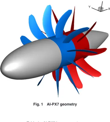
The open rotor test case is the AI-PX7 configuration, pictured in Fig.1. This is a generic open rotor designed by Airbus [33] and used to test, validate, and develop numerical approaches, within the Clean Sky JTI-SFWA European project in terms of CFD tech-niques and mesh requirements, and enhance the understanding of the complex aerodynamics around CROR. The geometry is an 11" 9 bladed pusher configuration with a rotor diameter of D¼ 4.2672 m (14 ft). Inlet and exhaust are not modeled in the na-celle shape. Table 1 gives a short overview of the AI-PX7 configuration features in high-speed conditions.
The blade geometry used in this paper is a blade with a sweep function varying from negative value at low radius to positive val-ues up to the tip, as shown in Fig.4. The transonic blades need to be swept to decrease the magnitude of the shock structure. The blade has a low thickness-to-chord ratio, similar to current tran-sonic fan blades, and low camber throughout its span. The rear rotor diameter is reduced by 10% relative to the front blade while the rear blade chord is increased in order to generate a thrust of equivalent magnitude for both rotors. The rear rotor cropping ena-bles us to decrease the impact of tip vortices convected from the front rotor to the rear rotor.
The nacelle design corresponds to a transonic nacelle design with the objective of minimizing as much as possible the local Mach number seen by the blades. The flow is, thus, only slightly accelerated by the front part of the nacelle. In high-speed condi-tions, Mach number increases from 0.73 in the freestream to 0.75 just upstream of the front rotor. The nacelle designs used inelsA andENSOLV simulations for the comparison are slightly different (see Fig.2). Considering that the maximum cross section of both
Fig. 1 AI-PX7 geometry
Table 1 AI-PX7 key parameters
Geometrical parameters Value Blade number (BF" BR) 11" 9
Front rotor diameter,D (m) 4.2672 Rear rotor cropping (%) 10 Rotor-rotor spacing,s (m) 0.95 Performances parameters at high-speed Value Freestream Mach number, M1 0.73 Front rotor rotation speed,XF(rpm) #795
Rear rotor rotation speed,XR(rpm) 795
Advance ratio,J 3.83 Angle of attack,a 1 deg
nacelles are very close and drive the acceleration of the incoming flow, it is assumed that these geometrical differences have a negligible impact on the in-plane forces.
4
Open Rotor Meshing
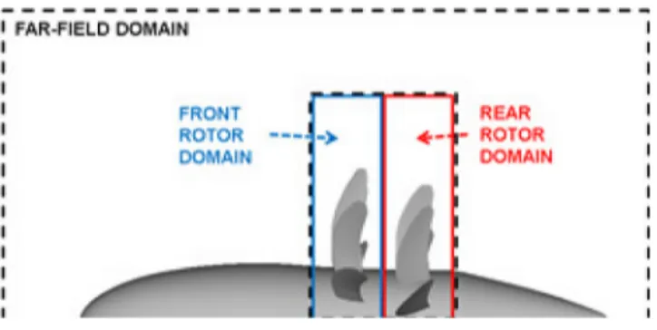
An open rotor configuration is composed of fixed parts (front and rear parts of the nacelle) and rotating parts (front rotor) and contra-rotating parts (rear rotor). This leads to a split of the mesh into three distinct domains: one far-field fixed mesh and two
cylindrical rotating meshes (one for each rotor), pictured in Fig.3. Each rotor mesh is contained in a cylindrical domain. This enables us to refine the mesh around the blade areas without any propaga-tion of refined mesh into the far-field area. This mesh strategy is also suitable for the modeling of installation effects on aircraft.
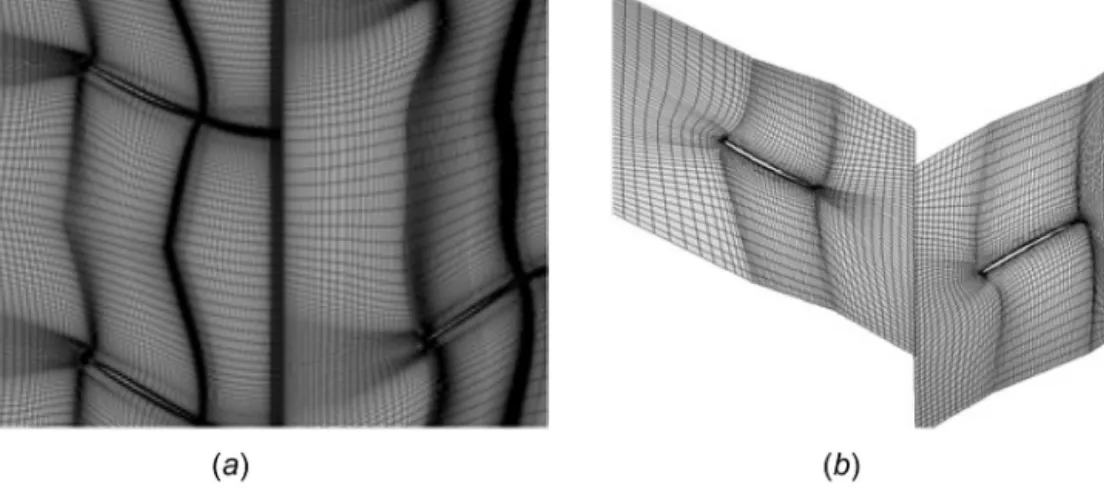
4.1 Grid Density. For elsA computations, the whole mesh contains around 53" 106 nodes. The far-field mesh contains 5" 106nodes. The front and rear rotor meshes contain 26.5 and 21.5" 106 nodes, respectively. The periodicity in each rotor is fully exploited for the mesh. Each rotor can be split into channels. For each channel, the blade is meshed by a C-block. H-blocks sur-round the C-block to complete the channel. The front blade con-tains 69 points on the chord direction and 86 points in the spanwise direction (see Fig.4). The rear blade contains 113 points on the chord direction and 82 points in the spanwise direction. The blade-to-blade passage contains 75 points in the azimuthal direction (see Fig.5). The axial mesh density is higher on the rear blade in order to capture unsteady wake effects from the front blade. To capture accurately the boundary layer on the blades and nacelle, 25 points are used, with ayþaround one in the first cell.
For theENSOLV computations, the whole mesh contains around 3.7" 106nodes. The far-field mesh contains 1.7" 106nodes. The front and rear rotor meshes contain 1.1 and 0.9" 106nodes, respec-tively. The blade surface resolution is 40 cells in the chord direction
Fig. 2 Two different Airbus nacelle designs for AI-PX7 configuration
Fig. 3 Splitting of the computational domain
and 22 cells in the spanwise one. The blade-to-blade passage con-tains 48 points in the azimuthal direction. For the blade topology, one row of O-blocks surrounds the blade. To capture accurately the boundary layer on blades, 16 points are used, with ayþaround two
in the first cell. This is followed by H blocks to fill up the channel. Grid density features of both meshes are gathered in Table2. Table 2 also highlights the ratio of density between the two meshes. The mesh density ratio is defined as the ratio between the number of nodes inelsA and ENSOLV for a domain (front, rear, far-field)2or a specific direction (chord, span). Larger discrepan-cies are observed in the spanwise direction, in which the elsA mesh is about four times more refined. This is partly due to the nonmodeling of the boundary layer of the nacelle with the NLR mesh. Mesh size discrepancies in the chord and azimuthal direc-tions for blades are more moderate with a ratio of around 1:6. These grid densities were chosen for each code with regard to their best practices and their numerical setup, especially with respect to the order of the spatial numerical schemes used.
4.2 Sliding Mesh Technique. Unsteady full annulus computa-tions of open rotors rely on moving grid techniques. To achieve this, the sliding mesh technique is used for both computations. The sliding mesh technique is based on the use of nonconforming grid systems having different relative motions. A sliding surface can be defined as the boundary between two nonconformed meshes. Nonconforming meshes have been first used with fixed meshes in order to optimize the size of structured mesh [34] and ease the generation of meshes for complex geometry [35]. This technique has been extended to
grids with different relative motions. A recent industrial application was the aerodynamic simulation of a multistage compressor [36]. However, sliding mesh implementations differ forelsA and ENSOLV codes and are detailed below.
InelsA, the communication through the sliding surface is per-formed using a distribution of fluxes through the nonmatching interfaces, which rigorously ensures conservativity for planar interfaces. More details on the implementation and use of the slid-ing mesh technique with theelsA code can be found in the work of Fillola et al. [35] and Gourdain et al. [36].
InENSOLV, the fluxes are computed using the flow states in one row of dummy cells. The flow states in the dummy cells are interpo-lated using bilinear interpolation techniques. The interpolation coeffi-cients are based on the cell face center coordinates on each side of the sliding interface. A recent application of the sliding mesh tech-nique with theENSOLV code can be found in Laban et al. [19].
5
Comparison and Analysis of Results
This section presents the results of theelsA and ENSOLV simu-lations. Rotor forces, blade forces, and pressure distributions over different azimuths are compared. Forces on the nacelle are not considered here because this nacelle is a simple design used for test and validation of aerodynamic methods and is not representa-tive of a nacelle used for flight (no air intake or outlet). Thus, only forces on the blades will be analyzed. The reference axes and angles used in this paper are shown in Fig.6. Azimuthal angles hF;Rwill be counted positively in the rotation direction.
5.1 Rotor Forces
5.1.1 Definitions. First, the forces applied on a whole rotor stage are analyzed and compared. The global forces are obtained
Fig. 5 Blade to blade mesh: (a) elsA and (b) ENSOLV Table 2 Comparison of grid densities
Grid density (number of points) Density ratio elsA ENSOLV
elsA ENSOLV Computational domain Far-field 5.M 1.7M 1.423
Front rotor 26.5M 1.1M 2.853
Rear rotor 21.5M 0.9M 2.853 Front rotor Blade chord 69 40 1.72
Blade-to-blade azimuth 75 48 1.56 Blade span wise 86 22 3.90 Rear rotor Blade chord 113 40 2.82 Blade-to-blade azimuth 75 48 1.56 Blade span wise 82 22 3.72
Boundary layer 25 16 1.56
2The mesh density ratio is here expressed to the third power to give an average
by summing up all the contributions of the blades for each rotor. Rotor forces are split into the component along the rotation axis, commonly called thrust, and the component in the propellers plane called in-plane forces (here, YZ-plane). In-plane forces can then be decomposed with projection on the reference axis in which vertical and side components are used. This decomposition of the in-plane forces is commonly found in many works in the lit-erature [12,13,21] because the projection on the aircraft axis is straightforward. However, a modulus/angle decomposition (FIP,wIP) is preferred in this work because aerodynamic
mecha-nisms behind each term can be separated. ModulusFIPand angle
wIPare then defined as follows:
FIP¼ ffiffiffiffiffiffiffiffiffiffiffiffiffiffiffiffiffi F2 Yþ F2Z q ; wIP¼ arctan FY FZ " # (1)
By convention,wIP is oriented in the rotation direction for each
rotor stage. Nondimensional thrustCTand in-plane force modulus
CIPare used. CT¼ T q1n2D4 ; CIP¼ FIP q1n2D4 (2)
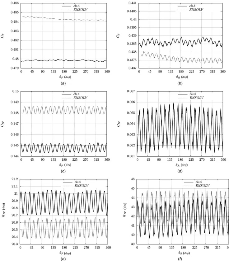
5.1.2 Comparison. Figure 7 presents thrust, nondimensional in-plane forces modulusCIP, and anglewIP for each rotor stage
(only blades are accounted for). The rotor thrust shows an almost-steady signal over a rotation. Fluctuations are negligible for the front stage and very low for the rear blade (magnitude is around 0:1% relatively to the mean value). Mean thrust mismatches between elsA and ENSOLV results are very small (<1% for the front rotor and< 0:3% for the rear rotor).
The CIP signal describes a periodic evolution with a
peak-to-peak fluctuation lower than 1% for the front rotor and around 6% for the rear rotor. These fluctuations are due to the aerodynamic interactions between rows. A meanCIP mismatch between elsA
andENSOLV simulations is observed on the front rotor (discrep-ancies around 2%) while it matches well on the rear rotor. Corre-lations between codes are observed as well on the mean anglewIP
for the front rotor (0.5 deg) and for the rear rotor (1 deg). The same magnitude of fluctuations due to the aerodynamic
interactions is captured by both codes (0.5 deg for the front rotor and 3 deg for the rear rotor).
To conclude, this comparison shows consistent results for both codes on rotor forces.
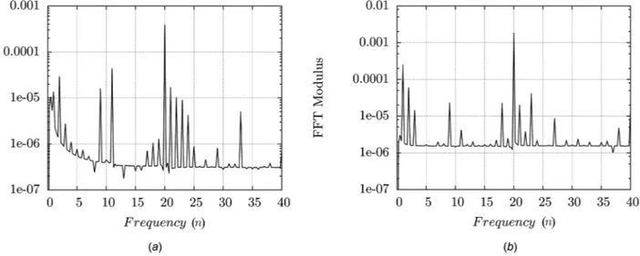
5.1.3 Fourier Analysis. A fast Fourier transform (FFT) is applied on theCIPsignal for both rotors over four complete
rota-tions in the absolute frame and presented in Fig.8. Given the time step used, frequencies above 40n are not considered here since they are not sampled accurately (less than 18 points in the period). According to the framework proposed by Tyler and Sofrin [37], rotor/rotor interactions give rise to frequencies characterized in the absolute frame of reference byhFBFnþ hRBRn, where hFand
hRare relative integers,B is the blade number, and n is the
rota-tion speed. For both rotors, a major peak arises at a frequency of 20n (hF¼ 1; hR¼ 1Þ. The front rotor FFT presents secondary
peaks of one of order of magnitude less than the major peak for frequencies of 2n (1,–1), 9n (0,1), and 11n (1,0). The rear rotor FFT shows secondary peaks for frequencies 1n (5,–6), 9n (0,1). The frequency of 1n is unexpected because the harmonics involved are high. This frequency may be nonphysical and due to a lack of convergence.
The peak magnitudes for the rear rotor spectrum are approxi-mately one order of magnitude higher than the ones from the front rotor. This highlights that the wakes play a major role in the aero-dynamic interactions.
5.2 Blade Thrust. The comparison now focuses on the local thrust of one blade, which is key data to understand and validate in-plane forces predictions. Figure9compares the thrust level of one blade (from each rotor) over one rotation for both computa-tions at an angle of attack of 1 deg. The thrust level fora ¼ 0 deg is also shown to highlight the effect of a nonzero angle of attack. The blade thrust signal emphasizes two aerodynamic phenomena with widely separated frequencies: the aerodynamic interactions and the effect of a nonzero angle of attack. This latter effect is characterized by a frequency equal to the frequency of rotation while aerodynamic interactions frequency, in the relative frame of reference, are the blade passing frequencies (BPFF,BPFR). The
variation of the thrust due to the effect of a nonzero angle of attack over one rotation is very important with regard to the mean thrust compared to the variations simulated with a zero angle of
attack (Fig.9). The peak-to-peak thrust variation represents about 60% of the mean value for the front blade whereas it represents 30% for the rear blade. Fluctuations due to the aerodynamic inter-actions seem to vary depending on the blade loading.
Figure 9also highlights the good matching for both computa-tions. The effect of a nonzero angle of attack can be observed as the overall shift of the polar towards the (90 deg, 180 deg) quad-rant, and aerodynamic interactions manifest as high frequency oscillations on the curve. Discrepancies appear for the maximum blade loading, in which the thrust level is slightly higher with
ENSOLV than elsA on the front blade and slightly lower for the rear blade. Both codes predict a maximum thrust value for each rotor athF& 120 deg for the front blade and hR& 135 deg for the
rear blade.
5.3 KpDistributions. The pressure distributions are
com-pared to verify the local behavior of the flow at specific radii. The nondimensional pressure coefficient Kp specific to propellers is
used and defined as follows:
Fig. 7 Global forces on rotors: (a) thrust coefficient on the front rotor, (b) thrust coefficient on the rear rotor, (c) in-plane force modulus on the front rotor, (d) in-plane force modulus on the rear rotor, (e) in-plane force angle on the front rotor, and (f ) in-plane force angle on the rear rotor
Kp¼1 p# p1 2q1ðV 2 1þ ðrXÞ 2 Þ (3)
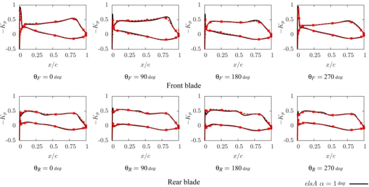
Figure10presents a comparison of theKpdistributions for the
ra-dius (n ¼ r=R ¼ 0:75). This radius was chosen because the blade develops the main part of its thrust in the area fromn ¼ 0:70 to the tip, and this section is often analyzed in literature. The aim is to observe how both codes capture the local flow physics around the blades. Various azimuthal positions are shown here.
Figure 10 presents good correlations between the elsA and ENSOLV results. In Fig.10, small differences appear mostly on the suction side where the pressure is rising (#Kpdecreases), in
particu-lar in the last quarter of the chord where a shock structure is visible. 5.4 Discussion. The comparison of several key aerodynamic flow features from two computations performed with two different codes (elsA, ENSOLV), on two different meshes (grid density, size of the computational domain), with two different numerical set-tings (turbulence model, spatial scheme, far-field, and nacelle boundary conditions) shows very consistent results for the global integrated forces. Locally, only minor discrepancies are observed, such as the shock highlighted by Kp distributions analysis (see
Fig.10), and they remain sufficiently low not to modify the global
forces. This good match also suggests that the boundary layer on the nacelle has a limited impact on the global forces.
Table3gathers the global forces averaged over a full rotation for both solvers. The influence of the grid density with theelsA code is also presented. For theENSOLV code, the study on the grid density for open rotors simulations has already been per-formed but on a different case. This previous study has shown that doubling the grid density in the three directions modifies by less than 1% the global forces as compared to the current grid density used here. For the elsA, comparisons with a coarser grid (one point over two in each direction for the Euler mesh, 25 nodes are kept to ensureyþ¼ 1 on the wall, which gives a total amount of
9M of points) show differences on global forces compared to the current grid. Rotor thrust predicted with the coarse grid is under-estimated by 3% and 5% compared to the current grid, respec-tively, for the front and rear stage. Oddly, in-plane force modulus difference and angle difference for the front stage are much smaller (1%) whereas the rear angle difference is around 5%. For this application, the elsA code requires a finer grid density than theENSOLV code to reach the mesh convergence. The mesh size used withENSOLV seems to be sufficient to get the global forces. The fourth-order space discretization used inENSOLV contributes partly to reach the mesh convergence with fewer points compared to theelsA code, for which a second-order scheme is used.
Fig. 8 Fast Fourier transform on CIPsignal from elsA computations: (a) front rotor and (b) rear rotor
As both simulations were performed with different turbulence models, an additional simulation was performed with the elsA code on the coarse grid with thek#x turbulence model to mea-sure its impact on the in-plane forces prediction. Comparison of these results with the Spalart–Allmaras ones highlights discrepan-cies around 1% for the front stage. The rear stage in-plane force modulus remains quasi-unchanged while thrust coefficient and angle increase by 1% and 2%, respectively. Consequently, the influence of the turbulence model has the same order of magni-tude as the discrepancies observed between the two codes.
To conclude, this comparison highlights consistent and encour-aging results (the maximum discrepancies are below 2%) and is a promising step in the verification process of prediction tools. Ex-perimental measurements would be an excellent way to consoli-date the reliability of these results. Altogether, the consistency of the results builds enough confidence to perform a deeper analysis of the physics behind in-plane forces in the following section.
6
Understanding the Physics Behind In-Plane Forces
This section aims at understanding the physics behind the in-plane forces. First, an in-depth analysis of the phenomena contrib-uting to in-plane forces applied to the front rotor is investigated. Second, the same analysis is performed on the rear stage. Based
on this analysis, differences between in-plane forces from front and rear rotors are discussed. This section presents only the results performed with theelsA code.
6.1 Understanding the In-Plane Force on the Front Rotor. For the front rotor, the aerodynamic simulation on the AI-PX7 configuration at high-speed at an angle of attack of 1 deg predicts a mean in-plane force modulus of 30:0% with respect to its rotor thrust and a mean angle of 20.8 deg. This section details the mech-anisms contributing to the modulus and the direction of the in-plane force. First, a quick reminder of the freestream velocity effect will be given. Second, the influence of the induced velocity will be analyzed. Third, the impact of the potential effects from the opposite stage on the in-plane forces will be studied.
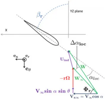
6.1.1 Freesrteam Velocity Effect. At zero angle of attack, the freestream velocity vector is perpendicular to the rotation plane of the propellers. With a nonzero angle of attack, its projection on the rotation plane leads to a nonzero vector and the velocity trian-gle is modified. The impact of the freestream velocity on the ve-locity diagram is called here the freestream veve-locity effect. Figure
11illustrates the velocity diagram for a propeller at nonzero angle of attack.W1represents the freestream velocity projected in the
propeller rotating frame and is defined as follows: W1¼ V1#rX eh
¼ V1cosa exþ ½V1sina sin h#rX)eh
(4)
The region between hF;R¼ 0 deg and hF;R¼ 180 deg is called
advancing blade whereas the other region is called retreating blade. In the advancing part, the angle of attack component V1sina is summed up to the rotating speed and contributes to an
increase of the local incidencealoc(see Fig.11). Thus, blades in
the advancing part generate more lift and drag, which means, by projection, more thrust and torque about the rotational axis. An opposite effect is obtained on the retreating part by symmetry. The projection of lift and drag on the propellers plane leads to an in-plane force with a zero angle.
6.1.2 Induced Effect. The flow circulation around the blades and the nacelle modifies the velocity field in the vicinity of these
Fig. 10 Kpdistribution on blade at n ¼ 0:75
Table 3 Average global forces sensitivities regarding the mesh size and the turbulence model
elsA ENSOLV Grid size Current (53M) Coarse (9M) Current (3.7M) Turbulence Model SA SA k#x k#x Front rotor CT 0.4804 0.4633 0.4676 0.4843 CIP 0.1447 0.1421 0.1430 0.1482 wIPðdegÞ 20.8 20.6 20.8 20.5 Rear rotor CT 0.4392 0.4176 0.4228 0.4376 CIP 0.06352 0.06369 0.06355 0.06356 wIPðdegÞ 41.7 39.9 40.5 42.9
areas. This phenomenon is defined as the induced effect. The flow circulation around the blades varies depending on the azimuthal position and, consequently, the analysis of the velocity triangle seen by the blade becomes much more complex than what was proposed in Fig.11. To evaluate this impact of the induced effect, the induced velocityUindis defined as the difference between the
velocityW and the freestream velocity W1 in the rotating frame
as follows:
Uind¼ W # W1
¼ uxexþuheh
(5)
Figure 12illustrates how induced velocities impact the velocity triangle. For a better understanding of the impact of the induced velocities on the flow, the variation of the local incidenceDalocis
introduced and defined as the oriented angleðW1; WÞ.
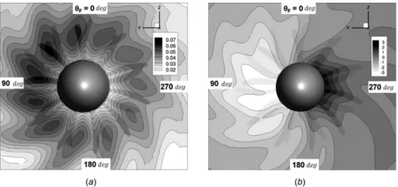
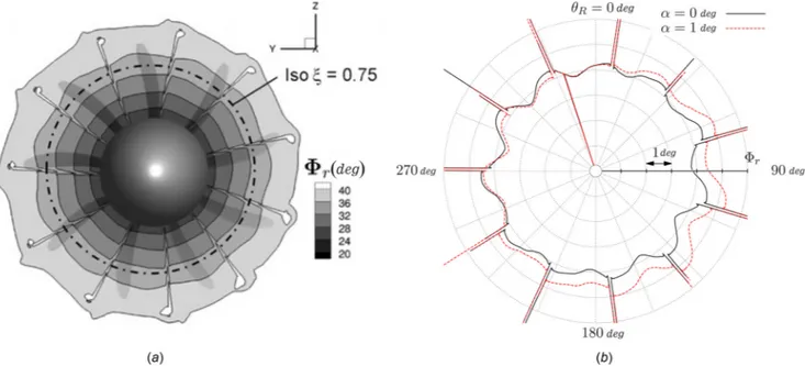
Figure13(a)displays the axial induced velocity fieldðux=Vx1Þ
estimated from CFD simulations on an X-plane cut at one
chord upstream of the front rotor. The axial induced velocity field is positive all over the disk because the front rotor generates suc-tion. Over a rotation, induced axial velocities around the blade-to-blade passage present maxima values in the angular area from approximately hF¼ 30 deg to hF¼ 120 deg, which is consistent
with the thrust variation on a single blade as seen in Fig.9. Blades on the advancing part generate more suction and, consequently, high axial induced velocity. Along the radial direction, axial induced velocity increases, reaching a maximum value around r=R¼ 0:75, and then decreases after. Axial induced velocities at hF¼ 0 deg are greater than those at hF¼ 180 deg. Ortun et al.
[21] show similar results with the HOST code on a single propeller.
To complete the analysis, Fig. 13(b) displays the change of local incidenceDalocdue to the induced effects on an X-plane cut
at one chord upstream of the front rotor. The positiveDalocvalue
means that the local incidence is increased by the induced effect. Areas around hF¼ 0 deg show a slightly lower value of Daloc
than in the areas aroundhF¼ 180 deg. Blade aerodynamic
load-ing is, consequently, higher for blade at hF¼ 180 deg than for
hF¼ 0 deg and contributes to the generation of the lateral
compo-nent of in-plane forces and, consequently, the in-plane force angle with the (Oz) axis. Areas of positive and negative extrema values of Daloc are centered on an axis driven by hF¼ 100 deg and
hF¼ 280 deg, respectively. The local incidence for the advancing
blade is strongly reduced by the induced effects whereas the one for the retreating blades is increased but to a lesser extent. The induced effect tends to decrease the difference between the maxi-mum and minimaxi-mum loading of the blade over a rotation and, con-sequently, to decrease the modulus compared to the case without induced effect (see Sec.6.1.1). The induced velocities present a nonsymmetric pattern between the positive half-plane and the z-negative one. Consequently, this distribution of induced velocities field contributes to get a nonzero anglewIP.
The influence of the induced velocities can be explained in a different way with an induced sideslip analogy. The joint analysis of the induced velocity field (Fig.13) and thrust variation of a sin-gle blade (Fig.9) shows that the advancing half on each rotor gen-erates more thrust and, consequently, more air suction (characterized by the axial induced velocity in Fig.13) than the retreating part. This induces momentum qvy from the retreating
half to the advancing half, which acts as if there was a sideslip angle. This induced lateral distortion creates a force in the lateral directionðOyÞ. Consequently, this lateral component gives a non-zero angle for the in-plane force.
Fig. 11 Velocity triangle for propellers at nonzero angle of attack: (a) front view of propellers and (b) advancing blade
Fig. 12 Velocity triangle for propellers at nonzero angle of attack with induced velocities
The induced effect contributes to both the angle and modulus for the in-plane force of the front rotor.
6.1.3 Impact of Aerodynamic Interactions. Potential effects from the rear rotor are seen in the front rotor frame of reference as temporal interactions characterized by the blade-passing fre-quencyBPFFand its harmonics. Their effect is noticeable on the
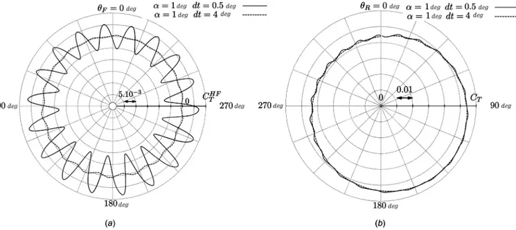
thrust of a single blade as described in Sec.5.2. A time step equiv-alent of 0.5 deg of rotor stage rotation enables us to sample the first harmonic of aerodynamic interactions with more than 30 points. To measure the impact of the aerodynamic interactions on the in-plane force predictions, larger time steps were used in order to degrade the capturing of these interactions and, thus, isolate their impact. Although this approach may have side-effects on the accuracy of the predictions, it provides an original way to nearly suppress aerodynamic interactions while retaining an unsteady framework suited to full annulus computation at nonzero angle of attack. Indeed, the frequency of propeller rotation, which mainly drives the effect of a nonzero angle of attack in the relative frame, is well captured for all the time steps because the largest time step used (dt¼ 4 deg) samples its period with 90 points.
Figure14presents the in-plane force modulus and angle for the front rotor. Variations ofCIPandwIPdriven by theBPFFand its
harmonics are not captured at all fordt¼ 4 deg. For dt ¼ 1 deg, variations are captured but with a slightly lower magnitude than
the case with dt¼ 0:5 deg but with a larger magnitude than the case withdt¼ 2 deg. Figure14(a)highlights that the aerodynamic interactions do not contribute to the mean in-plane force modulus. However, the angle wIP is more sensitive to the aerodynamic
interactions. The mean angle is overestimated by, respectively, 3.5 deg with the larger time step compared to the finer one. This difference is reduced to 0.5 deg with a time step of 1deg, which remains acceptable.
In short, potential effects do not contribute to the mean in-plane force modulus but to the angle. Results with a time step of 1 deg show acceptable matching for all the variables plotted compared to the finer time step.
To understand why the in-plane force direction is more sensi-tive to the aerodynamic interactions, the aerodynamic behavior of the opposite stage needs to be considered. As seen in Sec.5.2, the aerodynamic blade loading, characterized by the thrust coefficient, varies depending on its azimuthal position, which impacts the potential effects and wakes. To emphasize this coupling between the two stages, the aerodynamic loading of one single blade of each rotor is considered. Here, the impact from the rear stage to the front stage is analyzed. Thus, to quantify the aerodynamic interactions of the front blade, its thrust coefficient, expressed in the relative frame, needs to be filtered to keep only theBPFFand
its harmonics. Thus, these fluctuations can be isolated by filtering the low-frequency term linked to the frequency of rotation and
Fig. 13 Instantaneous induced velocity flow-fields in an X-plane at one chord upstream of the front rotor: (a) normalized axial induced velocity ux=Vx ‘ and (b)Daloc (deg) due to induced
velocity field
subtracting the mean value on theCTsignal. The termCHFT can be
introduced for measuring the impact of the aerodynamic interac-tions on the thrust coefficient. It gives
CHFT ¼ CT# CT# CLFT (6)
The low frequency componentCLF
T is driven by the rotation speed
of the rotor. This component can be modeled with a sinusoidal signal whose magnitude and phase are determined with a fast Fou-rier transform applied on theCT signal. Figure15(a)presents the
filteredCHF
T thrust coefficient on a front rotor single blade for two
time steps (dt¼ 0:5 deg, dt ¼ 4 deg) at angle of attack a ¼ 1 deg. First, as observed in the previous paragraph, almost no fluctuation is captured for the large time stepdt¼ 4 deg, and the filtered thrust coefficientCHF
T value is close to 0. Second, fordt¼ 0:5 deg, the
CHF
T signal can be modeled as a sinusoidal signal whose magnitude
and phase vary with the azimuth. Figure15(b)completes the analy-sis by plotting the thrust coefficient of a single blade from the oppo-site stage. Joint analysis of Fig.15(a)and Fig.15(b)highlights that the magnitudes of the aerodynamic interactions on the front blade are influenced by the aerodynamic blade loading of the rear blade.
Both magnitudes of variations ofCHF
T and thrust coefficient value
of the rear blade reach their maximum in the area between hF¼ 180 deg and hF¼ 270 deg (or between hR¼ 90 deg and
hR¼ 180 deg). The energy of the upstream potential effects is
linked to the aerodynamic rear blade loading and explains the cou-pling. These azimuthal variations due to the aerodynamic interac-tions also contribute to modify the direction of the in-plane force.
6.2 Understanding the In-Plane Force on the Rear Rotor. For the rear rotor, the aerodynamic simulation on the AI-PX7 con-figuration at high-speed at angle of attack of 1 deg predicts a mean in-plane forces modulus of 14:4% with respect to its rotor thrust and a mean angle of 41.5 deg. The in-plane forces modulus of the rear rotor is reduced by a factor of 2.5 compared to the front rotor. The angle is also increased by 20 deg from front to rear stage. This section details the mechanisms contributing to the modulus and the direction of the in-plane forces. First, the increase of axial velocity due the front stage is studied. Second, the deflection of the flow due to the front stage is analyzed. Third, the impact of the potential effects and wakes on the in-plane forces is investi-gated in more depth.
Fig. 15 Impact of the aerodynamic interactions on a front single blade: (a) filtered thrust coefficient CHF
T on a front single blade and
(b) thrust coefficient CTon a rear single blade
Fig. 16 Impact of the increase of the axial velocity due to the front stage: (a) axial velocities on an X-plane at one chord upstream to the rear rotor and at n 5 0:75 and (b) velocity triangle for the advancing blade
6.2.1 Increase of the Axial Velocity. The front rotor generates thrust and, consequently, the axial velocity for the rear rotor is higher than the axial freestream velocity (see Fig.16(a)). Conse-quently, the impact of the projection of the freestream velocity in the propellers plane with the termV1sinðaÞ on the velocity
trian-gle is reduced and so is the variation of local incidencealoc(see
Fig.16(b)). This implies a reduction of the variation of blade load-ing over a rotation compared to the front stage, as shown by the rear blade thrust signal in Fig.9. The peak-to-peak magnitude of the rear signal is reduced by a factor of 2 as compared to the front one. The front rotor acts as a filter of the freestream velocity effect by decreasing its influence on the downstream rotor. Conse-quently, the mean increase of axial velocity contributes to decrease the in-plane force modulus.
The behavior of the propeller system is consistent with distor-tion processing in turbofans or multistage compressors, for which circumferential nonuniformities are reduced as the flow proceeds through the machine (see Ref. [38], for instance).
6.2.2 Swirl Effect. The deflection of the flow by the front rotor also generates an increase of the orthoradial velocity, which
is called the swirl. This directly impacts the relative flow angles Urseen by the rear rotor, defined as
Ur¼ arctan Wh
Vx
" #
(7)
Wh is the relative orthoradial velocity in the rear rotor rotating
frame and Vx is the axial velocity. The relative flow angle Ur
varies proportionally with the local incidencealocaccording to the
following equation:
Ur¼p
2# brþ aloc (8) Figure17(b)highlights that at a constant given radiusr, the rela-tive flow angle is higher for the blades betweenhR¼ 45 deg and
hR¼ 215 deg than on the opposite part. This orientation of the
field of relative flow angles directly impacts the direction of the in-plane force and leads to an angle of 45 deg. This observation is fully consistent with the rear blade thrust variation observed in Fig.9and with the in-plane force angle in Fig.7(f).
Fig. 17 Relative flow anglesUrðdegÞ upstream of the rear rotor: (a) X-cut at one chord upstream of rear rotor (a 5 1 deg) and (b)
extraction from a line at n 5 0.75
Figure17shows that the relative velocity deficit of the wakes from the front blade entails an increase of the local incidence on the rear blade, which is just the consequence of the velocity com-position. Wakes impacting the rear rotor contribute to the genera-tion of small fluctuagenera-tions on the global forces on the whole rotor. The next paragraph focuses on evaluating their impact on the in-plane force component (modulus, angle).
6.2.3 Impact of the Aerodynamic Interactions. Potential effects and wakes propagating downstream from the front rotor are impacting the rear rotor and are characterized by the blade-passing frequency BPFR and its harmonics. The same study as
performed for the front rotor in Sec.6.1.3is applied here to the rear rotor. Figure18shows the in-plane forces modulus and the angle over a rotation for the rear rotor. Similar observations made in Sec.6.1.3apply for the rear rotor. Aerodynamic interactions do not contribute to the mean in-plane force modulus but to the mean direction. Compared to the front rotor (see Fig.15), the variations forCIP andwIP are more important. Wakes are more energetic
than potential effects and, thus, have a stronger impact.
Then, the impact of the aerodynamic interactions on a rear sin-gle blade is studied. Figure19(a)presents the filtered thrust coeffi-cientCHF
T on a front single blade for two time steps (dt¼ 0:5 deg,
dt¼ 4 deg) at angle of attack a ¼ 1 deg. CHF
T was defined in Eq. (6). First, as observed in the previous paragraph, almost no fluctu-ation is captured for the large time stepdt¼ 4 deg, and the filtered thrust coefficientCHF
T value is close to 0. Second, the fluctuations
ofCHF
T are more important than those from the front rotor as seen
in Fig.15(a). Figure19(b)completes the analysis by plotting the thrust coefficient of a single blade from the opposite stage. Joint analysis of Figs.19(a)and19(b)draws similar conclusions as in Sec.6.1.3. A correlation can be established between the magni-tude of the fluctuations ofCHF
T for the rear rotor and the thrust
dis-tribution from the front one, but a phase-shift arises between the signals. High values ofCT are reached forhF¼ 120 deg whereas
high values of magnitude forCHF
T are reached athF¼ 45 deg (or
hR¼ 315 deg). The wake released from a front blade impacts a
rear blade located at a different azimuth, which may explain the phase-shift between the signals. These azimuthal variations due to the aerodynamic interactions contribute to modify the direction of the in-plane force.
7
Conclusions
In this paper, unsteady aerodynamic simulations of an isolated CROR at high-speed at a nonzero angle of attack have been
compared and analyzed. Results obtained on global integrated variables such as in-plane forces and thrust show good matching between the elsA and ENSOLV codes. Mean value and fluctua-tions are both well captured despite different computational do-main, grid densities, numerical setup, and turbulence models (the maximum discrepancies are below 2%). Analysis of pressure dis-tribution demonstrates that local discrepancies appear in the area of shock structures but have a very low impact on the global forces. Different grid densities used on the blade skin inelsA and ENSOLV simulations probably explain these discrepancies. The comparison highlights also that an accurate prediction of global variables (thrust, in-plane forces) is reached with a coarser mesh with ENSOLV (3:7M of points) compared to the mesh used for elsA simulations (53M of points) due to a smaller computational domain, the nonmodeling of the boundary layer on the nacelle, and a higher order space scheme. Simulations with coarser mesh (9M of points) were performed with elsA and present discrepan-cies on the global variables. Two turbulence models (Spalart– Allmaras,k#x) were also tested with elsA, and their influence on the global variables appears to have the same order of magnitude as the discrepancies observed between the two codes. To con-clude, the code-to-code comparison enables us to strengthen the confidence in the numerical results, which is a first step in the ver-ification process of in-plane forces prediction.
In the second part of this work, the physics behind in-plane forces was analyzed for both rotors separately. For the front rotor, the first key mechanism is the orientation of the freestream veloc-ity that generates different local incidences seen by the blades at different azimuths (freestream velocity effect). The second key mechanism is driven by the induced velocities, the magnitude, and the direction of which vary with the azimuth (induced effect). Both effects contribute to the modulus of the in-plane force, but only the induced effect is responsible for a nonzero in-plane force angle wIP. To a lesser extent, aerodynamic interactions have a
weak impact on the mean direction (few degrees) but no effect on its mean modulus. This contribution is explained by the nonhomo-geneous impact of the aerodynamic interactions regarding the azi-muthal position because potential effects energy depends on the aerodynamic rear blade loading. The physics behind rear rotor in-plane forces is more complex. The freestream velocity effect is still a major contributor to the in-plane forces but with a lesser magnitude compared to the front rotor. The front rotor behaves as a filter by increasing the mean axial velocities, which contributes to a decrease of the modulus. The second key mechanism is the swirl created by the front rotor that modifies the local incidence
Fig. 19 Impact of the aerodynamic interactions on a rear single blade: (a) filtered thrust coefficient CHF
T on a rear single blade
seen by the rear blades, which increases the anglewIP. Wake
con-vection, in addition to potential effects, decrease the mean angle by a few degrees but do not affect the mean modulus. Wakes energy depends also on the aerodynamic front blade loading and their impact on the rear blades vary depending on its azimuth location.
This work offers a better validation and understanding of the in-plane forces for an isolated open rotor and can be extended to more complex applications for which in-plane forces play an im-portant role such as whirl flutter and installed configurations applications.
Acknowledgment
This work is funded by Airbus, in the framework of CleanSky JTI-SFWA European project. The authors are particularly grateful to Airbus for permitting the publication of this paper, and wish to thank F. Blanc, R. Collercandy, F. Magaud, M. Montagnac, and C. Negulescu for their advice and help in the development of this work.
Nomenclature
BF¼ number of front blades
BR¼ number of rear blades
BPFF¼ blade-passing frequency of the front rotor,
BPFF¼ 2 " n " BR(Hz)
BPFR¼ blade-passing frequency of the rear rotor,
BPFR¼ 2 " n " BF(Hz)
CT¼ thrust coefficient, CT¼ T=q1n2D4
CHF
T ¼ high frequency component of the thrust coefficient
CIP¼ in-plane forces modulus coefficient,
CIP¼ FIP=q1n2D4
D¼ front propeller diameter (m) dt¼ timestep (deg/iteration)
ex,er,eh¼ basis vectors of the rotating frame
FIP¼ in-plane forces modulus, FIP¼
ffiffiffiffiffiffiffiffiffiffiffiffiffiffiffiffiffi F2
Yþ F2Z
p
(N) FY;Z¼ lateral, normal force component (N)
J¼ advance ratio
Kp¼ nondimensional pressure coefficient
M1¼ freestream Mach number
n¼ frequency of propeller rotation (1/s) p1¼ freestream pressure (Pa)
r¼ radius (m)
R¼ radius of the front blade (m) s¼ rotor-rotor axial spacing (m) T¼ thrust (N)
ux¼ axial induced velocity (m/s)
uh¼ orthoradial induced velocity (m/s)
V1¼ freestream velocity (m/s)
Vx1¼ X-component of the freestream velocity (m/s)
W1¼ freestream velocity projected in the front
rotor rotating frame (m/s)
yþ¼ nondimensional size of the first cell
from the wall
Greek Symbols
a ¼ angle of attack between the propellers axis and free stream velocity (deg)
aloc¼ local incidence for a given propeller blade at a given
radiusr (deg)
br¼ pitch angle of blade at r=R (deg)
hF;R¼ azimuthal position of a given blade for front/rear
rotor (deg)
n ¼ relative radius, n ¼ r=R q1¼ freestream density (kg/m3)
wIP¼ angle of in-plane forces with (Oz) axis (deg)
UR¼ relative flow angle at r=R (deg)
X ¼ propeller rotation speed (rad/s)
Acronyms
CFD¼ computational fluid dynamics CROR¼ contra-rotating open rotor
DTS¼ dual time stepping
LUSSOR¼ lower upper symmetric successive over relation SA¼ Spalart–Allmaras
URANS¼ unsteady Reynolds-averaged Navier–Stokes WTT¼ wind tunnel testing
References
[1] Hager, R. D., and Vrabel, D., 1988, “Advanced Turboprop Project,” NASA SP Technical Report No. 495.
[2] Lanchester, F. W., 1916,The Flying-Machine From an Engineering Standpoint, Constable and Co., London.
[3] Harris, R. G., 1918, “Forces on Propeller Due to Sideslip,” British Aeronautical Research Council, Technical Report No. 427.
[4] Glauert, H., 1919, “The Stability Derivatives of an Airscrew,” British Aeronaut-ical Research Council, TechnAeronaut-ical Report No. 642.
[5] Glauert, H., 1935,Aeroplane Propellers, Miscellaneous Airscrew Problems, (Aerodynamics Theory, Vol. IV), Springer, New York.
[6] Goett, H. J., and Pass, H. R., 1941, “Effect of Propeller Operation on the Pitch-ing Moments of SPitch-ingle-Propellers Monoplanes,” NACA Technical Report No. L-761.
[7] Ribner, H. S., 1945, “Propellers in Yaw,” NACA Technical Report No. 820. [8] Bober, L. J., Chaussee, D. S., and Kutler, P., 1983, “Prediction of High Speed
Propeller Flows Fields Using a Three-Dimensional Euler Analysis,” NASA TM Technical Report No. 83065.
[9] Wong, P., Maina, M., Forsey, C. R., and Bocci, A. J., 1988. “Single and Contra-Rotating High-Speed Propellers: Flow Calculation and Performances Prediction,” ICAS No. 2.4.2.
[10] Nicoud, D., Brochet, J., and Goutines, M., 1989, “A Methodology Proposal to Design and Analyse Counter-Rotating High Speed Propellers,” ASME Paper No. 89-GT-38.
[11] Denton, J., and Singh, U. K., 1979, “Time Marching Methods for Turbomachi-nery Flow Calculation,”Application of Numerical Methods to Flow Calcula-tions in Turbomachines (VKI Lecture Series), E. Schmidt, ed., von Karman Institute for Fluid Dynamics, Rhode-St-Genese, Belgium.
[12] Nallasamy, M., 1994, “Unsteady Blade Pressures on a Propfan: Predicted and Measured Compressibility Effects,”J. Aircr.,31, pp. 730–736.
[13] Bousquet, J.-M., and Gardarein, P., 2002, “Improvements on Computations of High Speed Propeller Unsteady Aerodynamics,”Aerosp. Sci. Technol.,7(6), pp. 465–472.
[14] Stuermer, A., 2008, “Unsteady CFD Simulations of Contra-Rotating Propeller Propulsion Systems,” 44th AIAA/ASME/SAE/ASEE Joint Propulsion Confer-ence and Exhibit, Hartford, CT, July 21-23,AIAAPaper No. 2008-5218. [15] Zachariadis, A., and Hall, C. A., 2011, “Application of a Navier–Stokes Solver
to the Study of Open Rotor Aerodynamics,”ASME J. Turbomach.,133(3), p. 031025.
[16] Peters, A., and Spakovszky, Z. S., 2012, “Rotor Interaction Noise in Counter-Rotating Propfan Propulsion Systems,” ASME J. Turbomach., 134(1), p. 011002.
[17] Schnell, R., Yin, J., Voss, C., and Nicke, E., 2012, “Assessment and Optimiza-tion of the Aerodynamic and Acoustic Characteristics of a Counter Rotating Open Rotor,”ASME J. Turbomach.,134(6), p. 061016.
[18] Stuermer, A., and Yin, J., 2011, “Installation Impact on Pusher-CROR Engine Low Speed Performance and Noise Emission Characteristics,” 46th Applied Aerodynamics Symposium of Rotating Bodies, Orleans, France, March 28-30. [19] Laban, M., Kok, J. C., and Prananta, B. B., 2010, “Numerical Tools for
Contra-Rotating Open-Rotor Performance, Noise and Vibration Assessment,” 27th International Congress of the Aeronautical Sciences (ICAS 2010), Nice, France, September 19-24.
[20] Brandvik, T., Hall, C., and Parry, A. B., 2012, “Angle-Of-Attack Effects on Counter-Rotating Propellers at Take-Off,”ASMEPaper No. GT2012-69901. [21] Ortun, B., Boisard, R., and Gonzalez-Martino, I., 2012, “Assessment of
Propel-ler 1P-Loads Predictions,”Int. J. Eng. Syst. Model. Simul.,4, pp. 36–46. [22] Dequin, B., Kampa, A. M., Grunhagen, K., Basset, P. M., and Gimonet, B.,
2000, “HOST: A General Helicopter Tool for Germany and France,” 56th An-nual Forum of the American Helicopter Society, Virginia Beach, VA, May 2-4. [23] Cambier, L., Heib, S., and Plot, S., 2013, “The OneraelsA CFD Software: Input
From Research and Feedback From Industry,”Mech. Ind.,14(03), pp. 159–174. [24] Kok, J. C., 2000, “Resolving the Dependence on Freestream Values for thek–x
Turbulence Model,”AIAA J.,38, pp. 1292–1294.
[25] Kok, J. C., 2009, “A Higher-Order Low-Dispersion Symmetry-Preserving Finite-Volume Method for Compressible Flow on Curvilinear Grids,”J. Com-put. Phys.,228, pp. 6811–6832.
[26] Jameson, A., Schmidt, R. F., and Turkel, E., 1981, “Numerical Solutions of the Euler Equations by Finite Volume Methods Using Runge-Kutta Time Stepping,”AIAAPaper No. 1981-1259.
[27] Jameson, A., 1991, “Time Dependent Calculations Using Multigrid, With Appli-cations to Unsteady Flows Past Airfoils and Wings,”AIAAPaper No. 91-1596. [28] Spalart, P. R., and Allmaras, S. R., 1992, “A One-Equation Turbulence
Trans-port Model for Aerodynamic Flows,” 30th AIAA Aerospace Sciences Meeting and Exhibit, Reno, NV, January 6-9,AIAAPaper No. 92-0439.
[29] Yoon, S., and Jameson, A., 1987, “An LUSSOR Scheme for the Euler and Navier–Stokes Equations,”AIAA J.,4, pp. 36–46.
[30] Jameson, A., and Yoon, S., 1986, “Multigrid Solution of the Euler Equations Using Implicit Schemes,”AIAA J.,24(11), pp. 1737–1743.
[31] Couaillier, V., 2005, “Effective Multidimensional Non-Reflective Boundary Condition for CFD Calculations Applied to Turboengine Aeroacoustics Pre-diction,” ISABE 17th Symposium on Air Breathing Engines (ISABE 2005), Munich, Germany, September 4-9.
[32] Boisard, R., Delattre, G., and Falissard, F., 2011, “Assessment of Aerodynamics and Aero-Acoustics Tools for Open Rotors,” 9th European Turbomachinery Conference, Istanbul, Turkey, March 21-25, pp. 21–25.
[33] Negulescu, C. A., 2013, “Airbus AI-PX7 CROR Design Features and Aero-dynamics,” SAE 2013 AeroTech Congress & Exhibition, Montreal, Canada, September 24-26,SAEPaper No. 2013-01-2245.
[34] Rai, M., 1986, “A Conservative Treatment of Zonal Boundaries for Euler Equa-tion CalculaEqua-tions,”J. Comput. Phys.,62, pp. 472–503.
[35] Fillola, G., Le Pape, M.-C., and Montagnac, M., 2004, “Numerical Simulations Around Wing Control Surfaces,” 24th International Congress of the Aeronauti-cal Sciences (ICAS 2004), Yokohama, Japan, August 29-September 3. [36] Gourdain, N., Montagnac, M., Wlassow, F., and Gazaix, M., 2010,
“High-Per-formance Computing to Simulate Large-Scale Industrial Flows in Multistage Compressors,”Int. J. High Perform. Comput. Appl.,24(1), pp. 429–443. [37] Tyler, J. M., and Sofrin, T. G., 1962, “Axial Flow Compressor Noise Studies,”
SAE Trans.,70, pp. 309–332.
[38] Purwanto, A., Deconinck, T., Vilmin, S., Lorrain, E., and Hirsch, C., 2011, “Efficient Prediction of Nacelle Installation Effects at Take-Off Conditions,” 9th European Turbomachinery Conference, Istanbul, Turkey, March 21-25.