Trajectory-Based Supplementary Damping Control
for Power System Electromechanical Oscillations
Da Wang, Mevludin Glavic, Senior Member, IEEE, and Louis Wehenkel
Abstract—This paper considers a trajectory-based approach to determine control signals superimposed to those of existing controllers so as to enhance the damping of electromechanical os-cillations. This approach is framed as a discrete-time, multi-step optimization problem which can be solved by model-based and/or by learning-based methods. This paper proposes to apply a model-free tree-based batch mode Reinforcement Learning (RL) algorithm to perform such a supplementary damping control based only on information collected from observed trajectories of the power system. This RL-based supplementary damping control scheme is first implemented on a single generator and then several possibilities are investigated for extending it to multiple generators. Simulations are carried out on a 16-generators medium size power system model, where also possible benefits of combining this RL-based control with Model Predictive Control (MPC) are assessed.
Index Terms—Supplementary damping control, reinforcement learning, extremely randomized trees, model predictive control.
I. INTRODUCTION
S
OME characteristics of modern large-scale electric power systems, such as long transmission distances over weak grids, highly variable generation patterns and heavy loading, tend to increase the probability of appearance of sustained wide-area electromechanical oscillations. These oscillations threaten the secure operation of power systems and if not con-trolled efficiently can lead to generator outages, line tripping and even large-scale blackouts [1], [2].The typical model-based design of damping controllers of electromechanical oscillations normally begins with the recognition of oscillation modes, then proceeds to determine controller parameters producing better damping performances and robustness, and ends with the verification via time-domain simulations [1], [3]. The control rules and parameters are usu-ally calculated based on local information and objectives, and remain “frozen” in practical application. In recent researches on electromechanical oscillations, some remote information reflecting global dynamics is introduced as additional inputs to local damping controllers so as to enhance their performances of damping inter-area oscillations [4]–[6].
However, increasing uncertainties brought by the renew-able generation, and the growing complexity resulting from new power flow control devices, make the robustness of this typical design approach become questionable. Moreover, the controllers scattered into different areas and installed at different moments need to be further coordinated so as to The authors are with the Department of Electrical Engineering and Computer Science, University of Li`ege, Belgium. E-mails: [email protected], [email protected], [email protected].
obtain satisfactory global performances. Improper combination of diverse controllers could indeed potentially deteriorate the damping level of electromechanical oscillations [2].
The ultimate goal of all efforts to design, coordinate, and adapt damping controllers is to make the controlled system dynamics better meet the requirement of damping electrome-chanical oscillations.
In this respect, and in order to adapt and coordinate multiple controllers, this paper proposes a trajectory-based supplemen-tary control superimposed on the existing damping controllers (Power System Stabilizers (PSS), Thyristor Controlled Series Capacitors (TCSC), and so on). The proposed method treats damping control as a discrete-time, multi-step optimal control problem. At a sequence of measurement times, it collects current system measurements, and based on these latter, it de-termines supplementary inputs to be applied at the next control time to existing damping controllers. The approach consists of using a RL framework in order to obtain the maximum control return over a given temporal horizon. The objective of damping electromechanical oscillations can be achieved by defining a particular control return. For example, one can define the control return of a sequence of supplementary damp-ing inputs as the negative distance between angular speeds and the rated angular speed over a future temporal horizon. Maximizing the return will force angular speeds to return and remain near the rated speed, and when all generators run at this speed, oscillations are damped. Thus, optimization of these supplementary inputs brings adaption and/or coordination to the existing damping controllers without the need for changing their own structure and parameters.
Different with other works using RL for oscillations damp-ing [7]–[11] where Q-learndamp-ing or some of its variants have been suggested, we use a model-free tree-based batch mode RL algorithm [12]–[14]. Furthermore, we propose to design a multi-agent system of heterogeneous non-communicating RL-based agents through separate sequential learning of individual agents [15], [16]. In addition, along some suggestions of the work in [12], our work explores possibilities to combine the proposed RL-based control with MPC.
The rest of this paper is organized as follows: Section II discusses basic elements of trajectory-based supplementary damping control, Section III describes the used tree-based batch mode RL method; our test system and simulation results are given in Section IV, and finally Section V offers some con-clusions and directions for future research. Three appendices collect technical details abut models and algorithms used in our experiments, so as to enable their reproducibility.
II. TRAJECTORY-BASED SUPPLEMENTARY CONTROL In this part, the proposed trajectory-based supplementary damping control is introduced in terms of feasibility, overall principle, mathematical formulation of the control objective, solution approaches and implementation strategy.
A. Feasibility
The feasibility of the proposed method derives from the following advances in power systems’ technology, machine learning, and large-scale optimization.
• Dynamic and real-time measurements: Wide-Area
Mea-surement System (WAMS) can provide real-time and synchronized information about system dynamics, espe-cially the information closely related to the recognition of oscillation modes and the improvement of global damping performances [17]–[19];
• Future response prediction: if a system model is available, future response of power systems can be approximately modeled; if not, the return over an appropriate temporal horizon of one damping control can be learned from the observation of power system trajectories in similar conditions, and then used to approximately predict the effect of controls on the future system response;
• Efficient algorithms: model-based methods and
learning-based methods [20]–[22] have evolved a lot in the last twenty years by exploiting ongoing progress in terms of optimization and machine learning algorithms.
B. Overall principle of the proposed method
The power system is considered in this work as a discrete-time system (power system dynamics are continuous in essence, but in our framework we consider discrete-time dynamics). Its trajectories are considered as time evolution of state variables of the controlled system. If the system model is available in the form:
xt+1= f (xt, ut), (1)
then it is possible to compute all future system dynamics by iterating (1), and based on them optimize control policies. In (1), xt is a state vector consisting of elements of the state
space X, and utis an input vector whose items are elements
of action space U (random disturbances can be considered as actions).
If the system model is not available, then its trajectories can still be recorded by using a real-time measurement system.
In both cases constraints on states and actions can also be incorporated by restricting the set of possible states and by restricting the actions that are possible for individual states.
Using certain supplementary inputs, we can force system dynamics to evolve approximately along the desired trajec-tories in which oscillations are damped, while taking into account random disturbances, prediction inaccuracy, measure-ment errors, and so on. This is the underlying concept of trajectory-based damping control.
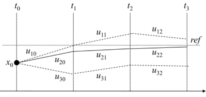
This idea is illustrated in Fig. 1, which describes three possible angular speed trajectories of one generator. From an
t0 t1 t2 t3 time ref x0 u10 u31 u12 u22 u32 u21 u11 u20 u30
Fig. 1. Trajectory based supplementary damping control
initial state x0, the angular speed will evolve along a path p
under a control sequence (up0, up1, up2, ..., p = 1, 2, 3). The
target is to search a particular sequence of discrete supple-mentary inputs to the damping controller on this generator (exciter or PSS), in order to drive its angular speed to return to the reference, and remain close to the reference as much as possible, like path 2 in Fig. 1 (plain line).
So, the key of trajectory-based supplementary damping control is to search a correct and exact sequence of discrete supplementary inputs (up0, up1, up2, ...). Here, the meaning of
“correct” is that calculated supplementary inputs can make system dynamics evolve along the desired trajectory deter-mined by a particular control objective, like the path 2 in Fig. 1. The meaning of “exact” is that there are not too large errors between decision-making scenarios and real system dynamics, like large measurement errors and model errors. If there are too large scenario errors, it may not be possible to find a control sequence yielding good damping effects in practice.
C. Control problem formulation
When system states move from xtto xt+1after applying an
action ut, a bounded reward of one step rt∈ R is obtained.
The definition of rtis closely related to the control objective.
As far as damping electromechanical oscillations is concerned, the negative distance between the angular speed vector wgand
the rated angular speed vector wref is defined as rt:
rt= −
Z t+1
t
|wg− wref|dt. (2)
Starting from an initial state xt and applying a sequence
of supplementary inputs (ut+0, ut+1, ..., ut+Th−1), the dis-counted return RTh
t over a temporal horizon of Th is defined
as: RTh t = Th−1 X i=0 γirt+i, (3)
where γ ∈ [0, 1] is the discount factor, and i = 0, 1, 2, ..., Th−
1. The sequence of actions ut+i is computed by a control
policy π mapping states to actions. A Th-step optimal policy
π∗ is one that maximizes RTh
D. Model-based vs model-free solution methods
Depending if dynamic models are available in analytical form, or if control returns from past trajectories are available in numerical form, the solution to the Th-step optimization
control problem of (3) is divided into two categories: model-based methods and model-free learning-model-based methods. Two approaches naturally fit this type of problems: MPC as model-based and RL as model-free.
1) Model Predictive Control (MPC): MPC is based on a
linearized, discrete-time state space model given by: ˆ
x[k + 1|k] = Aˆx[k|k] + B ˆu[k|k]; ˆ
y[k|k] = C ˆx[k|k]. (4)
Details of the power system model used in this work are provided in Appendix A. The future dynamics over a temporal horizon of Th is obtained by iterating (4):
ˆ y[k + 1|k] ˆ y[k + 2|k] .. . ˆ y[k + Th|k] = Pxx[k|k] + Pˆ u u[k|k] u[k + 1|k] .. . u[k + Th− 1|k] , (5)
where Px and Pu are given by,
Px= CA CA2 .. . CATh , Pu= CB 0 . . . 0 CAB CB . . . 0 .. . ... . .. ... CATh−1B CATh−2B . . . CB .
The return function of (3) is adapted as: RTh t = Th−1 X i=0 (ˆy[k + i + 1|k] − yr)TW (ˆy[k + i + 1|k] − yr) (6) which is minimized subject to linear inequality constraints:
umin≤ u[k + j|k] ≤ umax, j = 1, ..., Tc,
zmin ≤ z[k + i + 1|k] ≤ zmax, i = 1, ..., Th,
(7)
where yr is a vector of target values, z is a vector of
constrained operation variables like currents or voltages, W is weighting matrix, and Tc is control horizon (usually set
equal to or less than prediction horizon Th). This yields a
typical quadratic programming problem, which can be solved by active set or interior point methods [20].
MPC works as follows: at a control time, based on current measurements, calculate a sequence of optimal supplementary inputs minimizing the objective function (6) over a given temporal horizon. Only the first-stage control of the sequence is applied. The above steps are repeated at subsequent control times and continuously update these supplementary inputs.
2) Reinforcement Learning (RL): If the analytical system dynamics and return functions are unknown, one can still solve the problem by learning the map of system states to control actions using observations collected through a real-time measurements. This problem is naturally set as Markov Decision Problem (MDP) with the use of RL to learn the control policy. The use of system trajectories as time evolution
of all system state variables is problematic, in this context, because of the so-called ”curse of dimensionality” problem [21] and/or limitations in the measurement system.
The approach adopted in this work is to design a set of RL controllers (agents) acting on some system elements (generators) through learned mapping of its states (in the form of a single system state variable or a combination of several system state variables) to local control actions along the system trajectories. Consequently, an RL agent considers trajectories of its state and overall system behaviour results from collective actions of individual RL agents. The states of these RL agents is to be clearly differentiated from the system state and we therefore denote the RL states by s.
Given a set of trajectories represented in the form of samples of four-tuples (st, ut, rt, st+1), a near-optimal control policy is
a sequence of control actions minimizing the discounted return (3). This policy can be determined [9], [10] by computing the so-called action-value function (also called Q-function) defined by:
Q(st, ut) = E{rt(st, ut) + γ max ut+1
Q(st+1, ut+1)}, (8)
and by then defining the optimal control policy as: u∗t(st) = arg max
ut
Q(st, ut), (9)
as described in section III.
3) Discussion about solutions: MPC is a proven control technique with numerous real-life applications in different engineering fields, in particular process control [20]. The efforts applying MPC to damp electromechanical oscillations have been reported in [6], [23], [24]. However, in the present work, we focus on the RL approach to damp electromechanical oscillations. RL-based control of TCSC for oscillations damp-ing has been proposed in [9]. In [8], RL is applied to adaptively tune the gain of the conventional PSS. The use of RL to adjust the gains of adaptive decentralized backstepping controllers has been demonstrated in [11]. Wide-area stabilizing control, exploiting real-time measurements provided by WAMS, using RL has been introduced in [7].
Notice that both model-based or learning-based approaches usually find only suboptimal solutions due to the non-convexity of practical problems, modeling errors, randomness and limited quality of measurements.
While Q-learning based approaches have been proposed in previous works about oscillations damping [7]–[11], in the present work we propose to use a model-free tree-based batch mode RL algorithm to optimize supplementary inputs to existing damping controllers [14]. This choice is motivated by the following reasons [12]–[14]:
• This algorithm outperforms other popular RL algorithms on several nontrivial problems [12];
• It can infer good policies from relatively small samples of trajectories, even for some high-dimensional problems;
• Using a tree-based batch mode supervised learning tech-nique [13] it solves the generalization problem associated with RL techniques in a generic way [12], [14].
D C L sT sT K + + 1 1 ∑ KA Exciter R sT + 1 1 ∑ RL controller RL sT + 1 1 ∑ ∑ 2 2 1 1 d n sT sT + + 1 1 1 1 d n sT sT + + w pss w sT G sT + 1 1 Efmax Efmin Efd Vsmax Vsmin Vpmax Vpmin + + − + − Voltage Regulator Vref VLS
Terminal Voltage Limiter
ET
+ +
Power System Stabilizer
ω Δ
Other Signals
+ −
Fig. 2. Supplementary damping control
E. Implementation strategy
The proposed trajectory-based control scheme is not in-tended to replace existing damping controllers, but rather to optimize some supplementary control signals and superimpose them on the outputs of existing damping controllers so as to improve damping effects. In this way, the adaptation and/or the coordination of these existing controllers is implicitly achieved. The implementation considered in this work is illustrated in Fig. 2. For a given generator, the supplementary controller adds its control signal at the output of the PSS of the generator; it uses as inputs the angular speed of the generator and possibly other remote signals such as active power flows over tie-lines, so as to help damping of oscillation modes other than local ones.
At a control time, such a controller collects inputs and then it calculates the supplementary control signals so as to maximize the control return over a future temporal horizon.
III. TREE-BASED BATCH MODERL
The tree-based batch mode RL method that we propose to use calculates in an iterative way an approximation of the optimal Q-function over a temporal horizon of Thfrom a set of
dynamic and reward four-tuples (st, ut, rt, st+1) (observe the
state stat time t, take an action ut, receive the next state st+1
and the instantaneous reward rt) [14]. It has two components:
the extra-tree ensemble supervised learning method and the fitted Q iteration principle [14].
A. Extra-Tree ensemble based supervised learning
The supervised learning algorithm named Extra-Trees [13] builds each tree from the complete original training set. To determine a splitting at a node, it selects K cut-directions at random and for each cut-direction, a cut-point at random. It then computes a score for each of the K cut-directions and chooses the one that maximizes the score. All state-action pairs related to the node are split into the left subset or the right subset according to the chosen splitting. The same procedure is repeated at the next node to be split. The algorithm stops splitting a node until stopping conditions are met.
Three parameters are associated to this algorithm: the num-ber M of trees to be built to compose the ensemble model,
the number K of candidate cut-directions at each node and the minimal leaf size nmin. Inputting a state-action pair, each
extra-tree outputs a Q value by averaging all samples’ Q in the finally reached leaf node, and the output of an ensemble of extra-trees is the average of outputs of all extra-trees. To make this text self-contained the extra-trees algorithm is detailed in Appendix B.
B. Fitted Q iteration principle
The fitted Q iteration algorithm calculates an approximation of the Q-function over a given temporal horizon by iteratively extending the optimization horizon:
• At the first iteration, it produces an approximation of Q1
-function corresponding to a 1-step optimization. Since the true Q1-function is the conditional expectation of
the instantaneous reward given by the state-action pair (i.e., Q1(st, ut) = E{rt|(st, ut)}), an approximation of
it can be constructed by applying a batch mode regression algorithm, namely an ensemble of extra-trees whose inputs are state-action pairs (st, ut) and whose outputs
are instantaneous rewards rt.
• The N -th iteration derives an approximation of QN
-function corresponding to a N -step optimization horizon. The training set at this step is obtained by merely refreshing the outputted returns of the training set of the previous step by:
ˆ QN(st, ut) = rt(st, ut) + γ max ut+1 ˆ QN −1(st+1, ut+1) (10) Details about the tree-based batch mode RL are given in [14]. Once we have the ˆQTh(st, ut) function, an approxima-tion to the optimal return funcapproxima-tion over a Th-step optimization
horizon, we can use it to make damping control decision: for a state st, calculate all candidate actions’ expected return by
using the function ˆQTh(st, ut), and select the action with the largest one as supplementary input to the existing controller. Details of fitted Q iteration algorithm, as applied for the problem studied in this work, are given in Appendix C.
IV. TEST SYSTEM AND SIMULATION RESULTS
In this part, the tree-based batch mode RL on a single generator and multiple generators is investigated together with the combined control effects between MPC and RL, all in the same medium size power system model [1].
A. Test system
The one-line diagram of the test system is shown in Fig. 3. The Power System Toolbox (PST) [25] is used to simulate the system responses. A PSS is assumed on each generator. The system is composed of two areas: A1 and A2, which are connected through tie-lines 1-2 and 8-9. In the tests included in this work, a temporary three-phase short-circuit to ground at bus 1 (cleared by opening the tie-line 1-2 followed by its reconnection after a short delay) causes electromechanical os-cillations (local and inter-area). When controlled only through
G14 G1 G8 G3 G6 G13 G15 G11 G10 65 54 G4 G9 G7 G5 G2 G16 40 48 47 1 53 66 60 64 67 33 68 35 36 34 44 45 51 50 29 28 26 25 27 3 18 17 24 21 22 16 15 14 13 4 11 6 7 5 37 9 32 20 19 58 23 59 56 41 31 30 62 63 38 46 42 49 52 39 2 55 10 12 57 61 8 43 G12 TCSC 69 70 A1 A2
Fig. 3. 16 generators / 2 areas /70 buses test system
0 1 2 3 4 5 6 7 8 −3.8 −3.6 −3.4 −3.2 −3 −2.8 −2.6 −2.4 Time (s) (pu) with RL without RL 0 1 2 3 4 5 6 7 8 0.999 0.9995 1 1.0005 1.001 1.0015 Time (s) (pu) with RL without RL
Fig. 4. Active power of line 1-2 (top); angular speed of generator 1 (bottom)
existing PSSs and TCSC the system exhibits poorly damped oscillations, as shown by dashed lines in Fig. 4 corresponding to the temporal evolution over a period of 8s of the power flow through line 1-2 and the angular speed of generator 1.
B. RL-based control of a single generator
1) Sampling four-tuples: to collect a set of four-tuples (st, ut, rt, st+1), 500 system trajectories of 8 seconds
un-der a series of random actions for different fault durations
ranging from 0.01 to 0.05 seconds (this provides different initial conditions for each trajectory) are simulated. Every 0.1 seconds after the disturbance, the current states of a selected generator are sampled and a random action from an action space [−0.015, 0.015] is applied. A candidate action space includes all possible supplementary inputs for the PSS on this generator. The action space is discretized at a step of 0.005. The system state st+1reached at next time is observed
and the one-step reward rt by (2) evaluated. All in all, 2500
simulations (each over 8 seconds) are run, and a total of about 200000 four-tuples are thus collected.
2) Building extra-trees: based on a four-tuple set, an extra-tree ensemble consisting of 100 extra-trees (M = 100) is built using the method of [14]. We use the following tree parameters: discount factor γ = 0.95; leave size nmin = 1; splitting
attribute number K = 7 (six generator state attributes and one action attribute).
3) Q greedy decision making: the Q approximation is
iteratively calculated over an optimization horizon. At each control time, a damping action is determined as follows: collect the current state of controlled generator, select an action from the action space [-0.015, 0.015] and then calculate the Q value of this state-action pair by recursively searching all 100 trees and averaging their outputs. All candidate actions at the current state are thus probed and the action with the largest Q value is selected as the optimal supplementary input to the PSS of the controlled generator.
Fig.4 displays system response (solid lines) when the tree-based batch mode RL is applied only on generator 1. We observe that the introduction of this single supplementary con-trol already improves the damping. Next, the same method is applied on generator 2 and 3, and similar further improvements in damping are observed, as shown on Fig. 5. Clearly, the use of different generators would produce different, and hopefully complementary contributions to oscillations damping. Notice, however, that the optimal placement of the supplementary controllers is not considered in this work.
C. RL-based control of multiple generators
Interaction among RL-based controllers is a key problem to be solved when using them on multiple generators. Design of RL controllers on multiple generators should thus be carefully approached, because good or optimal solution of each individual controller when acting alone does not imply good or optimal solution to the system when all the controllers act together. To ensure the design of multiple controllers, three approaches can be adopted:
• Learning each controller’s policy individually, in the
ab-sence of the other supplementary controllers, and benefit from the learned control policies by using them simul-taneously. While this approach does not ensure a good collective performance, it was nevertheless illustrated successfully in the previous section.
• Separate sequential learning of the controllers (agents): a sequence of random actions to a first generator is first applied in order to yield its training sample while using the current control strategy for all other generators; the
0 1 2 3 4 5 6 7 8 0.9994 0.9996 0.9998 1 1.0002 1.0004 1.0006 1.0008 1.001 Time (s) (pu) with RL without RL 0 1 2 3 4 5 6 7 8 0.9994 0.9996 0.9998 1 1.0002 1.0004 1.0006 1.0008 1.001 Time (s) (pu) with RL without RL
Fig. 5. Angular speeds of generator 2 (top) and generator 3 (bottom)
generator’s states are recorded and corresponding one-step rewards computed; this is repeated until enough four-tuple samples about this generator are obtained and a new control policy is determined for this generator. Subse-quently, the new control policy of this generator is used while applying the same sampling procedure on a second generator, and so on. In other words, one controller learns at a time and for each additional controller its working environment is considered to be the system together with all existing controllers that already learned to solve the task they are responsible for. In this way a multi-agent system of heterogeneous non-communicating agents [15], [16] is formed.
• Simultaneous asynchronous learning: four-tuple sets of all controlled generators come from the same trajectories and random actions are applied to multiple generators simultaneously to generate these trajectories.
We believe that the sequential (i.e. separate but coordinated) learning approach is most natural to create a well coordinated multi-controller system. This approach is illustrated in Fig.6.
The intuition behind this approach is as follows. Let us imagine that there are 100 individual controllers in the system acting together. If one intends to add one more controller it is reasonable to adapt this controller to the system together with
Power System Model Controller 1 Action 1 Observations 1 Reward 1 Environment for Controller 2 Controller 2 Action 2 Observations 2 Reward 2
Fig. 6. Separate sequential learning of controllers: 1 pass, in the order 1-2
0 1 2 3 4 5 6 7 8 −3.6 −3.4 −3.2 −3 −2.8 −2.6 −2.4 Time (s) (pu) RL on generators 1−3 RL on generator 1 0 1 2 3 4 5 6 7 8 −3.8 −3.6 −3.4 −3.2 −3 −2.8 −2.6 −2.4 Time (s) (pu) separate sampling simultaneous sampling without RL
Fig. 7. Active power flow in line 1-2: multi-generator RL with a single 1-2-3 pass sequential learning (top); separate sequential sampling vs simultaneous asynchronous sampling (bottom)
the already tuned other 100 controllers instead of re-learning all the 100 existing ones. Simulation results included in this section illustrate and support advantages of this intuition.
The top figure of Fig.7 compares the results when the batch mode RL is applied only on generator 1 and then together on generators 1, 2 and 3. We can see that more RL controllers bring indeed better damping effects.
0 1 2 3 4 5 6 7 8 −3.6 −3.4 −3.2 −3 −2.8 −2.6 Time (s) (pu) combined control RL MPC
Fig. 8. Active power flow in line 1-2 with RL-based control combined with MPC in a control center
Using the same number of four-tuples and the same extra-tree parameters, control effects of two ways (sequential vs asynchronous) of sampling are shown in the bottom figure of Fig.7, when the tree based batch mode RL is applied to generator 1-3. The RL based on simultaneous sampling performs better than the scheme only using existing PSSs and TCSC in the first 6 seconds, but it brings large oscillations in the last 2 seconds. However, when compared with the RL based on the separate sequential sampling, the damping effects of the asynchronously learned controllers are clearly worse.
Specifically, in the four-tuple samples obtained using the simultaneous sampling, the dynamics and rewards of a gen-erator are decided not only by the actions applied to itself, but also by the dynamics and actions of the other generators. However, when utilizing these samples to select an optimal action for one generator at a control time, real dynamics and actions of the two other generators are normally different from those of collected learning samples, because they then switch from random actions to their learned policy. This leads to the wrong estimation about the return of one action, and possibly the wrong choice of action, which may jeopardize combined control effects. However, in the sequential sampling scheme, the rewards of a generator only represent consequences of its own actions, given the already tuned control policy used by the other generators, and hence it should lead to an improvement in damping each time a new controller is retrained. We hence use this approach (with a single 1-2-3 pass).
Remark. We do not consider related problems of determin-ing optimal number of RL controllers and the effect of the order in which controllers are designed. These considerations are left for future research.
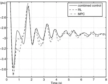
D. Combination of RL and MPC
The use of MPC to damp electromechanical oscillations has been investigated in our previous works [23], [24]. In this section, a possibility to combine control between MPC and the tree-based batch mode RL is further investigated. This possibility has been suggested in [12] through the comparison
of MPC and RL in a unified framework. The results of [12] show that RL may certainly be competitive with MPC even when a good deterministic model is available.
When MPC is infeasible due to the limits of communi-cations, measurements and models in real power systems, RL controllers based on local dynamics and rewards are set to complete MPC’s control effects. Here, we consider a combination of an MPC controller acting at the level of Area 2 control center to control generators 4-6 in this area with three RL-based controllers installed on generators 1-3 and obtained by sequential separate sampling (a single pass is used to train them in the order 1, 2, 3). The MPC state vector x includes generator, exciter, PSS, and turbine governor states. Output variables are angular speeds of generators 4-6. The input u is a vector of supplementary inputs for PSSs on generators 4-6, which is subject to −0.015 ≤ u ≤ 0.015. Prediction horizon of Th= 10 and control horizon of Tc= 3 steps are chosen. In the
objective function (6), all deviations of the predicted outputs from references are weighted uniformly and independently, i.e. W is the identity matrix. The MPC controller considers ±10% state estimation errors and a 0.05s delay. It updates every 0.1 seconds supplementary damping inputs for PSSs on generator 4-6. We refer the reader to [23], [24] for further details about the MPC scheme we use.
Figure 8 shows control response in terms of line 1-2 active power flow of the MPC controller alone, the RL controller alone, and when the two schemes are used in combination (while the RL-controllers have been trained with taking into account the effect of the MPC controllers on generators 4-6). We observe that the combined scheme indeed shows better performances with respect to the sole use of either MPC on generators 4-6 or RL on generators 1-3.
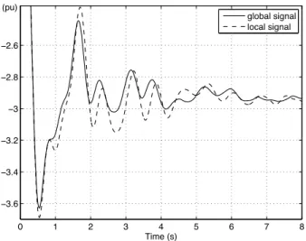
E. The use of a global signal
The proposed RL controller can also incorporate some remote information which represents, to some extent, system-wide dynamics to define its state, in order to enhance global control effects. The active power of tie-line 1-2 as global signal is introduced to the RL controller on generator 1, which is re-trained by repeatedly simulating system response under a series of random actions and collecting corresponding active power in line 1-2, while two other controllers (in generators 2 and 3) use local signals. Specifically, still considering the three-phase short circuit to ground at bus 1, RL controller on generator 1 collects active power of tie-line 1-2, and applies a random action every 0.1 seconds after the fault. At the next time, it collects the active power of line 1-2, and calculates the one-step instantaneous reward as:
rt= −
Z t+1
t
|p1−2− pref|dt, (11)
where p1−2is the controlled active power of line 1-2, and pref
is its reference which could be steady state exchange power before a disturbance, or a new post-disturbance exchange power determined by off-line simulations.
Fig. 9 displays the results when the RL controller installed on generator 1 uses global signal (solid line) while other
0 1 2 3 4 5 6 7 8 −3.6 −3.4 −3.2 −3 −2.8 −2.6 Time (s) (pu) global signal local signal
Fig. 9. Active power of line 1-2: global signal vs. local signal
two RL controllers use (generators 2 and 3) use local signal (solid line) and when all three RL controllers use local signals as inputs (dashed line). The local signal here means the generator angular speed. Better damping of the inter-area electromechanical oscillations is clearly observed with the RL controller installed on generator 1 using the global signal. This illustrates the flexibility of the proposed control in enhancing the damping of different oscillation modes by focusing on dominant ones depending on system prevailing conditions. F. Comparison with an existing method and performances in open-loop unstable case
Finally, the proposed RL supplementary control is compared with an existing damping control method, using the modal analysis from [1] as an example. All generators, except gener-ators 7 and 14, are assumed to have a PSS and their gains are optimized using root locus to obtain a damping ratio larger than 0.05, and the time constants are calculated according to the needed phase compensation. When a same three phase short circuit fault as above occurs, the response of active power in tie-line 1-2 is shown by the dashed line in Fig. 10.
Next, three RL-based controllers are installed on generators 1, 2, and 3. These controllers use the global signal of active power of tie-line 1-2. The solid line of Fig. 10 shows that the supplementary control signals on three generators could further improve the effects of existing controllers even if they are optimized in some way. Although the improvement is small, it is significant especially considering the difficulty of optimizing PSS parameters in practice.
Finally, in order to further illustrate damping effects of the proposed RL method we tested its performances in an open-loop unstable case (negatively damped low-frequency oscillations). The parameters of the PSS on generator 9 are first detuned in order to create such a scenario, as shown by the dashed line in Fig. 11. The RL-based controller, using active power of tie-line 1-2 as the global signal, is then installed on generator 9. The obtained result (solid line in Fig. 11) shows that the proposed RL controller works also quite efficiently in this unstable situation.
0 1 2 3 4 5 6 7 8 −3.1 −3 −2.9 −2.8 −2.7 −2.6 −2.5 −2.4 Time (s) (pu) with RL without RL
Fig. 10. Comparison with an existing method
0 1 2 3 4 5 6 7 8 −3 −2.8 −2.6 −2.4 −2.2 −2 Time (s) (pu) with RL without RL
Fig. 11. Control effects in unstable case (growing oscillations)
V. CONCLUSION
This paper proposed a trajectory-based supplementary damping control for electromechanical oscillations by directly controlling system dynamics with the help of additional con-trol signals. It does not replace existing damping concon-trollers. Rather, it superimposes its optimized control signals on the output of the existing controllers, so as to enhance their damping effects by exploiting remote measurements and/or by adapting the control strategy to changing system conditions.
The proposed supplementary damping control is treated as a discrete-time, multi-stage optimal control problem maximizing the control return over a given temporal horizon.
The paper focused on applying a tree-based batch mode RL method to learn supplementary damping controls from samples of observed trajectories. The results on a single generator show that the supplementary inputs calculated by using this method can further improve damping effects of existing controllers. When the tree-based batch mode RL on multiple generators is used, a separate sequential sampling and learning for each generator’s supplementary control is the most appropriate solution so as to effectively coordinate the different
supplementary controls. This method can also be combined with MPC to complete its control effects and cope with its modeling errors.
One of the main advantages of the learning-based strategy is that it does not rely on accurate analytical models of the system dynamics, but rather exploits directly measurements about the past performance of the system based on already observed system trajectories. It is therefore a promising approach to cope with the emerging features of power systems, whose dynamics more and more depend on the dynamics of loads and dispersed generation which incorporation into dynamic models would be a daunting task.
One practical problem about the tree-based batch mode RL approach is that it needs important computational resources to build and exploit large enough ensembles of extremely randomized trees. So, the future work would attempt to use some more efficient learning algorithms. Moreover, although RL implicitly considers the measurement and process noise at the learning stage by exploiting the system trajectories that include some noise, more work is needed to demonstrate the RL robustness in dealing with different types of process and measurement noises.
One essential advantage of the learning-based approach proposed in this paper is its very generic nature, so that it could be used even at the very local level of load and dispersed generation control, in order to “smarten” the whole power system control strategy at any layer.
ACKNOWLEDGMENTS
This paper presents research results of the Belgian Network DYSCO, funded by the Interuniversity Attraction Poles Pro-gramme, initiated by the Belgian State and of the PASCAL Network of Excellence funded by the European Commission. The scientific responsibility rests with the authors.
REFERENCES
[1] G. Rogers, Power System Oscillations, Kluwer Academic Publishers, 2000.
[2] E. Grebe, J. Kabouris, S. L. Barba, W. Sattinger and W. Winter, “Low frequency oscillations in the interconnected system of continental Europe,” in Proc. of IEEE Power and Energy Society General Meeting 2010, Minneapolis, MN, July, 2010.
[3] J. Turunen, J. Thambirajah, M. Larsson, et al, “Comparison of three electromechanical oscillation damping estimation methods,” IEEE Trans. Power Syst., vol. 26, no. 4, pp. 2398-2407, Nov. 2011.
[4] A. A. Hashmani and I. Erlich, “Mode selective damping of power system electromechanical oscillations using supplementary remote signals,” IET Gener. Transm. Distrib., vol. 4, no. 10, pp. 1127-1138, 2010. [5] R. Preece, J. V. Milanovi´c, A. M. Almutairi, and O. Marjanovic,
“Damping of inter-area oscillations in mixed AC/DC networks using WAMS based supplementary controller,” IEEE Trans. Power Syst., vol. 28, no. 2, pp. 1160-1169, May. 2013.
[6] R. Majumder, B. Chaudhuri and B. C. Pal, “A probabilistic approach to model-based adaptive control damping of interarea oscillations in power system,” IEEE Trans. Power Syst., vol. 20, no. 1, pp. 367-374, Feb. 2005. [7] R. Hadidi and B. Jeyasurya, “Reinforcement learning based real-time wide-area stabilizing control agents to enhance power system stability,” IEEE Trans. Smart Grid., vol. 4, no. 1, pp. 489-497, Mar. 2013. [8] R. Hadidi and B. Jeyasurya, “Reinforcement learning approach for
controlling power system stabilizers,” Canadian Journal of Electrical and Computer Engineering, vol. 34, no. 3, pp. 99103, 2009.
[9] D. Ernst, M. Glavic, and L. Wehenkel, “Power system stability control: reinforcement learning framework,” IEEE Trans. Power Syst., vol. 19, no. 1, pp. 427-435, Feb. 2004.
[10] M. Glavic, “Design of a resistive brake controller for power system sta-bility enhancement using reinforcement learning,” IEEE Trans. Control Syst. Technology, vol. 13, no. 5, pp. 743-751, Sep. 2005.
[11] A. Karimi, S. Eftekarnejad, and A. Feliachi, “Reinforcement learning based backstepping control of power oscillations,” Electric Power Sys-tems Research, vol. 79, no. 11, pp. 1511-1520, Nov. 2009.
[12] D. Ernst, M. Glavic, F. Capitanescu, and L. Wehenkel, “Reinforcement learning versus model predictive control: a comparison on a power system problem,” IEEE Trans. Syst. Man. Cyber., Part B: Cybernetics, vol. 39, no. 2, pp. 517-529, Apr. 2009.
[13] P. Geurts, D. Ernst and L. Wehenkel, “Extremely randomised trees,” Machine Learning, vol. 63, no. 2, pp. 3-42, Apr. 2006.
[14] D. Ernst, P. Geurts and L. Wehenkel, “Tree-based batch mode rein-forcement learning,” Journal of Machine Learning Research, vol. 6, pp. 503-556, Apr. 2005.
[15] S. Russell and P. Norvig, Artificial intelligence - A modern approach, Prentice Hall, 1995.
[16] P. Stone and M. Veloso, “Multiagent systems: A survey from a machine learning perspective,” Autonomous Robots, vol. 8, no. 3, pp. 345-383, 2000.
[17] A. G. Phadke and J. S. Thorp, Synchronized Phasor Measurements and Their Application, Springer, 2008.
[18] P. Korba and K. Uhlen, “Wide-area monitoring of electromechanical oscillations in the Nordic power system: practical experience,” IET Gener. Transm. Distrib., vol. 4, no. 10, pp. 1116-1126, 2010. [19] A. Chakrabortty, “Wide-area damping control of power systems using
dynamic clustering and TCSC-based redesigns,” IEEE Trans. Smart Grid., vol. 3, no. 3, pp. 1503-1514, Sep. 2012.
[20] J. M. Maciejowski, Predictive Control with Constraints, Prentice Hall, 2002.
[21] R. Sutton and A. Barto, Reinforcement Learning: an Introduction, MIT Press, 1998.
[22] L. Busoniu, R. Babuska, B. De Schutter, and D. Ernst. Reinforcement Learning and Dynamic Programming using Function Approximators, CRC Press, 2010.
[23] D. Wang, M. Glavic and L. Wehenkel, “A new MPC scheme for damping wide-area electromechanical oscillations in power systems,” in Proc. of the 2011 IEEE PES PowerTech, Trondheim, Norway, Jun. 2011. [24] D. Wang, M. Glavic and L. Wehenkel, “Distributed MPC of wide-area
electromechanical oscillations of large-scale power systems,” in Proc. of the 16th Intelligent System Applications to Power Systems (ISAP), Crete, Greece, Sep. 2011.
[25] J. H. Chow and K. W. Cheung, “A toolbox for power system dynamics and control engineering education and research,” IEEE Trans. Power Syst., vol. 7, no. 4, pp. 1559-1564, Nov. 1992.
[26] D. Wang, M. Glavic, and L. Wehenkel, “Comparison of centralized, distributed and hierarchical model predictive control schemes for elec-tromechanical oscillations damping in large-scale power systems,” Int. Journal of Elec. Power and Energy Syst., vol. 58, pp. 32-41, Jun. 2014. [27] P. Kundur, Power System stability and control, McGraw Hill
Profes-sional, New York, USA, 1994.
APPENDIXA
POWER SYSTEM MODEL
This section presents linearized models of relevant power system components used in MPC [25], [26]. The system state space equations are formed by combining the models of all dynamic devices and eliminating algebraic equations.
A. Generator dδ dt = ω Jdωdt = Pm− Pe− D∆ω Ψ00d =E 0 q(X 00 d−Xl)+Ψ1d(Xd0−X 00 d) X0 d−Xl − X 00 dId dΨ1d dt = 1 T00 d0 (E0 q− Ψ1d) dEq0 dt = 1 T0 d0 (Ef d− XadIf d) Ψ00 q = Ed0(Xq00−Xl)+Ψ1q(Xq0−X 00 q) X0 q−Xl − X 00 qIq dΨ1q dt = 1 T00 q0(E 0 d− Ψ1q) dE0d dt = − 1 T0 q0 XaqI1q XadIf d = (Xd0−X00 d)(Xd−Xd0) (X0 d−Xl)2 [E 0 q− Ψ1d +(Xd0−Xl)(Xd00−Xl) (X0 d−Xd00) Id] + fsat(Eq0) XaqI1q = (Xq0−X00 q)(Xq−Xq0) (X0 q−Xl)2 [E 0 d− Ψ1q +(X 0 q−Xl)(X00q−Xl) (X0 q−Xq00) Iq] + E 0 d (12)
where J is the moment of inertia; Pmis mechanical power; Pe
is electromechanical power; D is damping coefficient; Ψ00dand Ψ00q are d axis and q axis components of stator flux linkage; Ed0 and Eq0 are d axis and q axis transient stator voltages; Ψ1d
and Ψ1q are amortisseur circuit flux linkages; Xl is leakage
reactance; Xd, Xd0 and Xd00are d axis synchronous reactance,
transient reactance and subtransient reactance; Td00 and Td000 are open circuit time constant and open circuit subtransient time constant of d axis; Xq, Xq0 and Xq00 are q axis synchronous
reactance, transient reactance and subtransient reactance; Tq00
and Tq000 are open circuit time constant and open circuit
subtransient time constant of q axis; Idand Iq are d axis and q
axis stator currents; Xadand Xaq are mutual reactances; Ef d
and If d are excitation voltage and current; fsat is saturation
coefficient.
B. Exciter
Verr = Esig+ Vref+ Vpss− Vter dVR dt = KAVerr−VR TA dRf dt = −Rf+Ef d TF dEf d dt = VR−KEEf d TE (13)
where Verr is voltage deviation; Esig is supplementary input
signal; Vref is voltage reference; Vpss is output of PSS; Vter
is terminal voltage; VR and Rf are regulator states; KA and
TA are voltage regulator gain and time constant; KE and TE
are exciter constant and time constant. C. PSS dP SS1 dt = (P SSin−P SS1) Tw dP SS2 dt = (1−Tn1 Td1)GpssdP SS1dt −P SS2 Td1 dP SS3 dt = (1−Tn2 Td2) dP SS2 dt −P SS3 Td2 Vpss = TTn2 d2( Tn1 Td1Gpss dP SS1 dt + P SS2) + P SS3 (14)
where P SSin is the input of PSS, P SS1, P SS2, and P SS3
are PSS states; Gpssis PSS gain; Twis washout time constant;
Tn1 and Tn2 are lead time constant; Td1 and Td2 are lag time
constant. D. Turbine governor dT G1 dt = (T Gin−T G1) Ts dT G2 dt = (1−T3 Tc)T G1−T G2 Tc dT G3 dt = (T G2+T3TcT G1)(1−T4T5)−T G3 T5 Pm = T G3+TT4 5(T G2+ T3 TcT G1) (15)
where T Gin is the input of turbine governor; T G1, T G2 and
T G3 are state variables; Ts is servo time constant; Tc is HP
turbine time constant; T3is transient gain time constant; T4 is
time constant to set HP ratio; T5 is reheater time constant.
E. TCSC dXtcsc dt = KrT CSCin− Xtcsc Tr (16) where Xtcscis TCSC output; T CSCinis TCSC input signal;
Kris TCSC gain; Tr is its time constant.
Following the procedure of [27] the above differential-algebraic equations are reduced to a set of ordinary differential equations. The vector of system state variables is the com-bination of state variables describing each dynamic device, i.e. δt, ωt, Eq0t, Ψ1dt, E
0
dt, Ψ1qt, VR, Rf, Ef d, P SS1, P SS2, P SS3, T G1, T G2, T G3 and Xtcsc for the TCSC. The vector of
control variables includes supplementary control signals for each generator’s exciter and the TCSC.
APPENDIXB
EXTRA-TREE REGRESSION ALGORITHM[13]
Build a tree (T S)
Input: a training set T S, namely {(il, ol)}#Fl=1 Output: a tree T .
• If
1) #T S < nmin, or
2) all input variables are constant in T S, or 3) the output variable is constant over the T S. return a leaf labeled by the average value #T S1 P
lo l.
• Otherwise
1) Let [ij < tj]=Find a test (T S).
2) Split T S into T Sl and T Sr according to the test
[ij< tj].
3) Build from these subsets Tl = Build a tree(T Sl)
and Tr= Build a tree(T Sr);
4) Create a node with the test [ij < tj], attach Tl and
Tr as left and right subtrees of this node and return
Find a test (T S)
Input: a training set T S, namely {(il, ol)}#F l=1
Output: a test [ij < tj].
1) Select K inputs, {i1, ..., iK}, at random, without
re-placement, among all (non constant) input variables. 2) For k going from 1 to K:
a) Compute the maximal and minimal value of ik in
T S, denoted respectively iT S
k,min and iT Sk,max.
b) Draw a discretization threshold tk uniformly in
[iT Sk,min, iT Sk,max]
c) Compute the score Sk=Score ([ik< tk], T S)
3) Return a test [ij< tj] such that Sj= maxk=1,...,KSk.
An ensemble of M randomized regression trees is built by calling the function Build a tree M times on the original training set.
APPENDIXC
FITTEDQITERATION ALGORITHM[14] Inputs: a set F of four-tuples {(slt, u
l t, r l t, s l t+1)} #F l=1.
Output: an approximation ˆQ of the Q-function. Initialization:
Set N to 0.
Let ˆQN be a function equal to zero everywhere on X × U .
Iterations:
1) Repeat until stopping conditions are reached: a) N ← N + 1.
b) Build the training set T S = {(il, ol)}#F
l=1 based on
the function ˆQN −1 and on the set of four-tuples
F : il= (slt, ult), ol= rlt+ γ max u∈U ˆ QN −1(slt+1, u). (17) c) Use the regression algorithm to induce from T S
the function ˆQN(st, ut).
2) Return de function ˆQN
In our simulations we have st =
(δt, ωt, Eq0t, Ψ1dt, E
0
dt, Ψ1qt) and ut ∈ [−0.015, 0.015], when using only local signal. When using remote signals, these latter are added to the definition of st. The regression
algorithm is the Extra-Trees regression method.
Da Wang received the Ph.D. degrees respectively from the University of Shandong (China) and the University of Li`ege (Belgium) in 2009 and 2014. His research interests are in power system stability analysis and optimized control.
Mevludin Glavic received the M.Sc. and Ph.D. degrees from the University of Belgrade (Serbia) and Tuzla (Bosnia) in 1991 and 1997, respectively. His affiliations include: the University of Wisconsin- Madison (USA) as a Fulbright post-doctoral scholar, the University of Li`ege (Belgium) as senior research fellow and visiting professor, and Quanta Technology (USA) as senior advisor. He is presently a senior research fellow at the University of Li`ege. His research interests are in power system dynamics, stability, optimization, and real-time control.
Louis Wehenkel graduated in Electrical Engineering (Elec-tronics) in 1986 and received the Ph.D. degree in 1990, both from the University of Li`ege, where he is full Professor of Electrical Engineering and Computer Science. His research interests lie in the fields of stochastic methods for systems and modeling, optimization, machine learning and data mining, with applications in complex systems, in particular large scale power systems planning, operation and control, industrial process control, bioinformatics and computer vision.