Daniel M. Dubois
Department of Applied Informatics and
Artificial Intelligence, HEC Management
School, N1, University of Liège, rue
Louvrex 14, B-4000 Liège, Belgium
Stig C. Holmberg
ITM/Informatics
Mid Sweden University,
83125 Östersund, Sweden
Abstract
1In examining relationships between autopoiesis and anticipation in artificial life (Alife) systems it is demonstrated that anticipation may increase efficiency and viability in artificial autopoietic living systems. This paper, firstly, gives a review of the Varela et al [1974] automata algorithm of an autopoietic living cell. Some problems in this algorithm must be corrected. Secondly, a new and original anticipatory artificial autopoiesis algorithm for automata is presented. In our automata system, the asymmetric membrane of the self-creating living cell plays a central role. The simulation confirms the validity of our algorithm in showing its autopoietic properties.
1
Introduction
Autopoiesis, or self-organisation, is a concept first introduced in the early seventies by Francisco Varela and Humberto Maturana [Varela, 1996]. Furthermore, an original idea of the time was the computational model of an autopoietic living cell [Varela et al., 1974]. In this seminal paper they further argue that living systems belong to the class of autopoietic systems. However, if we in this context accept Rosen's [1985] quest that all living systems, even so artificial ones, are anticipatory systems, two evident questions will surface.
First, to what degree does the original model of Varela et al. [1974] represent the anticipatory properties of living systems?
Second, in what ways is it possible to modify the original algorithm in order to highlight the role of anticipation in the development of new living structures in the simulated system?
Hence, it is the main purpose of this paper to shred some light on the relationship between autopoiesis and anticipation in artificial life (Alife) systems.
1 CHAOS : Centre for Hyperincursion and Anticipation in Ordered Systems, Institute of Mathematics B37,
Grande Traverse 12, B-4000 Liège 1, Belgium http://www.ulg.ac.be/mathgen/CHAOS
2 Research
Approach
Starting from the original paper [Varela et al., 1974] we have identified two main research approaches.
First, a theoretical one making a critical evaluation of hitherto autopoietic research and raising fundamental questions about life, autopoiesis, and anticipation together with the relationships between them.
Second, a more pragmatic and practical research approach mainly accepting the assumptions of Varela et al. [1974] and just introducing anticipation into the original simulation algorithms from 1974.
In this paper we will mainly follow the second approach postponing most of the first approach to future ones. In so doing we will start with a discussion and assessment of a fairly broad sample of current research papers on autopoietic systems. With help of this survey we hope to shed light on our first research question.
Our approach in the second phase is experimental, integrative, and innovative. For the experimental part we use a web based simulation tool as our core vehicle. Hence our readers will become active participants in this research endeavour via their ordinary web browsers.
For the integrative part we will combine the research on autopoiesis and artificial life by Varela et al. [1974], Varela and McMullin [1997], and McMullin [1997] with our own research on anticipatory modelling, simulation, and computing [Dubois, 2003; Holmberg, 1998]. In this way we want to demonstrate that (artificial) living systems have not only robust autopoietic properties [McMullin and Varela, 1997] but also strong anticipatory ones.
Coming to the innovative part, at last, by involving a simulation tool we have already demonstrated that a highly creative and idea generating research milieu will emerge [Dubois and Holmberg, 2008].
3 Autopoietic
Research
Nearly innumerable derivations and combinations can be drawn from the autopoietic research published so far. Here, however, we will mainly focus on relations and connections between autopoiesis and computing anticipatory systems of interest for our first research question.
Varela himself said that his model of autopoiesis is a model of actual living cell. He said that his model does
not be applied to Artificial Life (Alife). Also, he wrote that a real autopoietic system can not be simulable on computer, even if he proposed an algorithm (sic).
Robert Rosen proposed his Metabolic-Repair model (M, R), similar to the autopoietic model of Varela. Rosen also claimed that his MR model is not computable.
But the lambda-calculus shows that autopoietic model are computable and simulable on a computer because this can be transformed to a general recursive system.
So, as stated in the title of our paper, we may speak about the “artificial autopoiesis”, which open new routes for Alife, but also for AI (Artificial Intelligence).
Francisco J. Varela [2000] related autopoiesis to cognition and proposed a biology of intentionality in relation to autopoiesis, and we may add that any intention is linked to an anticipation.
Robert Rosen [1985] believed that the distinction between matter and life is due to the property that living systems are anticipatory systems.
Anticipation will be a fundamental and included property in an autopoietic programmed system.
The rules of the Varela et al model algorithm are explicit instructions for the computer program which simulates the autopoiesis. The membrane, in this model, is semi-permeable to the substrate S, which only passes from the environment to the interior of the cell membrane. This cell is thus an open system to matter, the substrate S.
4
Original Algorithm of the Autopoietic
Automata
Varela et al. [1974] presented a simulation model showing how already a very simple system embedded in a two dimensional, discrete space, could exhibit autopoietic properties and develop and maintain a closed boundary. The algorithms, however, were a bit ambiguous and the software implementation obviously did not fully correspond with the text in the paper [McMullin, 1997].
So each cell in the system world, aside from being empty, may contain one of three different particles or elements:
S : Substrate K : Catalyst L : Link
Those entities are involved in three distinct reactions: SR1. Stochastic Composition: K + 2S → K + L If two substrate particles are directly adjacent to each other and to a catalyst particle they will produce a link particle, the catalyst particle remaining unaffected.
SR2. Stochastic Disintegration: L → 2S
This reverse reaction occurs stochastically for all link particles with a fixed probability per time step and link.
SR3. Stochastic Concatenation: Bonding Each L can form zero, one or two bonds:
L, L–, –L or –L–
In this way forming indefinitely long bonded chains: –L–L–L–L–
Also this is a stochastic reaction that may happen to any two adjacent link particles each of which has already either zero or one bond. The link chain (bonding) will
broke down only if or when constituent link elements disintegrate back to substrate particles when any associated bonds will also decay.
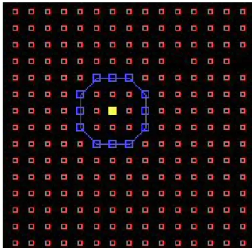
Here is an example of the initial configuration of the automata, given at Figure 1, in the Pascal program [Mingers et al., 1997]. Even with this initial configuration, given by a cell already constructed with a closed membrane and a catalyst in it, the Pascal program fails to obtain a correct dynamics of the autopoiesis.
Figure 1: Initial configuration of the Varela et al.
autopoiesis automata. The small open squares are substrates S, the set of bigger open squares with bonds to each other is the membrane formed with Links L, and the full square in the center of the cell is the catalyst K.
Indeed, a consistent failure of the autopoietic process is due to the spontaneous and premature bonding of the L particles, produced within the membrane, which become immobile and unavailable to repair the membrane.
Due to space restrictions, the complete improved and refined algorithm of McMullin [1997] will not be presented here.
It is however implemented, and explained, in our simulation model at www.c8systems.com/aaa/.
Important for our discussion here, however, is to observe that this algorithm is completely geared by random processes.
5
Anticipatory Extended Autopoietic
Automata Models
In looking at the algorithms, it is clear that these autopoietic models are too simple for realizing an actual living system.
The model is a 2D space automata system. A more realistic model would be a 3D space automata system, because an actual cell spherical membrane is 3D. A 2D circle cell membrane with 2 holes is no more a cell but 2 separated curved membranes. A 3D spherical cell membrane may have as many holes as possible without destroying its spherical topology.
The model is rather static in the sense that the cell is fixed in the automata. Actual cells are moving. Indeed, an actual living cell shows continuous internal and external dynamical movements.
There is no mechanism of reproduction in this model. Reproduction by cellular division would enhance the viability of this model. Indeed, in the real nature, any cell follows the classical destiny of all living system, by the successive process of birth, growth, and finally death.
The rules of this model are given by algorithmic instructions or commands not included in the autopoietic model. A full autopoietic model must include its own rules. These rules must be located in a memory. Indeed, it seems logic to consider that the main steps of the evolution of any living system, which is the result of the natural selection, must be embedded in them, in some memory blocks. When a living system grows, it develops itself with a reviving of the main successive steps of its evolution, which play the role of rules for its development.
A system for memorizing the rules must be defined. Indeed, the common aspect of any living system, even the virus, is the universal genetic code, which contains the program of the organization of the life. Within the memory, a pro-gram (the term pro-gram means a script which is written in advance) could be self-generating and self-producing, and self-evolving. What is extraordinary in the living world, is the fact that the self-programmed genetic code is universal in all living systems. Within any multi-cellular living organism, all the cells possess the same message of the genetic code, but the decoding of this message gives rise to different types of cells with different structures and functions.
The message of the genetic code is different in the different types of living systems. The genetic code is the main support of anticipation in living systems, because it is pre-programmed.
Robert Rosen [1985] gives the example of the simplest form of anticipation in living systems. It is an organism of just a few cells that tends to move toward dark places. This not because darkness provide any special benefits but due to the fact that dark places also tend to be humid. Humidity, in its turn, provides a favourable environment for the living organism. Hence, according to Rosen, that movement toward dark places is a sign of simple (pre-programmed) anticipatory behaviour.
The main modification we have done to Varela's original algorithm deals with the problem of the semi-permeable membrane with bonded links, which are symmetric. The semi-permeable membrane must be asymmetric, as defined in our anticipatory automata in the next section.
6 The Algorithm of the Anticipatory Autopoietic Automata
This section gives a new automata algorithm of anticipatory autopoiesis.
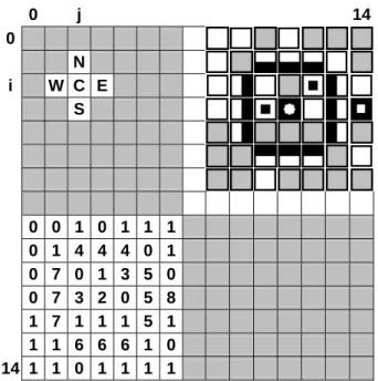
6.1 Structure of the Autopoietic Automata The automata system is given, in Figure 2, by a grid with 15 x 15 cells, as in the Varela et al. automata. At the upper left, an automaton cell, C, is linked to the North, East, South and West cells. At the lower left, the automata state numbers for a living cell. At the upper right, the automata state pictures for the same living cell.
0 j 14 0 N i W C E S 0 0 1 0 1 1 1 0 1 4 4 4 0 1 0 7 0 1 3 5 0 0 7 3 2 0 5 8 1 7 1 1 1 5 1 1 1 6 6 6 1 0 14 1 1 0 1 1 1 1
Figure 2: This figure shows the 15 x 15 cells of the
cellular automata.
The correspondence between the state number and the state picture is given in Figure 3.
Figure 3: Legends of pictures for representing the
different states of the automata.
Each cell C(i,j) is the line number i[0,14] and column j[0,14].
The boundaries of the automata are periodic: C(15,j)=C(0,j) and C(i,15)=C(i,0), simulating a space without border.
Each cell communicates with the 4 adjacent cells at North, N, East, E, South, S and West, W, as shown in the Fig. 2.
The content of a cell is identified by its state number: 0 is an empty cell E, 1 is the substrate S, 2 is the catalyst K, 3 is a link L, the set, 4, 5, 6, 7, are the north, east, south and west links LN, LE, LS, LW, and 8 is the disintegrating link DL.
This Fig. 2 also shows an autopoietic system, with a catalyst, 2, and a membrane identified by the north, east, south, and west links, LN=4, LE=5, LS=6, LW=7.
0 E Empty
1 S Substrate
2 K Catalyst
3 L Link
4 LN North bonded Link
5 LE East bonded Link
6 LS South bonded Link
7 LW West bonded Link
The 4 sides of the membrane are coded with a different state number, because it is necessary to identify which side of the membrane is semi-permeable to the substrates S: a substrate S at the North of the bounded link LN, will cross the membrane.
For example, at the north membrane, the possible transitions are given as follows:
E+LN+XE+LN+X, 04X04X, S+LN+EE+LN+S, 140041, S+LN+SE+LN+L, 141043, where X represents any state num
In our anticipatory autopoiesis, the disintegration of the membrane will be performed with a renewal of the membrane.
The bonded links, 4, 5, 6, 7, of the membrane will be replaced as, for example:
L+LE+EE+LE+LD, 350058
where LD is a disintegrating link, represented by the state number 8.
The disintegrating link LD decay, randomly, to 2 substrates S, if two empty cells are adjacent:
E+LD+ES+E+S, 080101
In the automata, the cells 0 and 1 are randomly interchanged at periodic time steps. The cells 8 and 0 are also randomly interchanged at periodic time steps. The cells 3 and 1 are randomly interchanged at periodic time steps.
6.2 Functions of the Anticipatory Algorithm The algorithm is structured with the following functions: 1. Initial configuration of the automata, with the following data.
1A. Each automaton is randomly defined as empty E(0) or contents a substrate S(1), with a percentage P(1)% which is chosen.
1B. One or several automata contain a catalyst K(2). 2. Iterative modifications of the automata states, with the following 10 successive steps.
2A. The catalyst K(2) creates the initial bonded links LN(4), LE(5), LS(6), and LW(7), if there are two adjacent substrates S(1). For example, the creation of the LN(4):
K(i+1,j)+S(i,j)+S(i1,j) K(i+1,j)+E(i,j)+LN(i1,j) 2B1. Passage of substrates S(1) across the semi-permeable bonded links LN(4), LE(5), LS(6), and LW(7). The bonded links LN(4) are semi-permeable to substrates S(1) only in one direction, from the North to the South, for LE(5), from the East to the West, for LS(6), from the South to the North, and for LW(7), from West to the East. For example, the passage of S(1) across a bonded link LN(4):
LN(i,j)+E(i+1,j)+S(i1,j) LN(i,j)+S(i+1,j)+E(i1,j) 2B2. Creation of a link L(3), from a first substrate S(1), and the passage of a second substrate S(1) across the bonded links LN(4), LE(5), LS(6), and LW(7), which are the catalysts of the links L(3). For example, creation of a link L(3), from a substrate S(1),and the passage of a second substrate S(1) across the bonded link LN(4): LN(i,j)+S(i+1,j)+S(i1,j) LN(i,j)+L(i+1,j)+E(i1,j)
2C. Transformation of adjacent links L(3) to bonded links LN(4), LE(5), LS(6), and LW(7). For example, transformation of a link L(3), adjacent to the East or West
of a bonded link LN(4), to bonded link LN(4): LN(i,j)+L(i,j+1) LN(i,j)+LN(i,j+1)
LN(i,j)+L(i,j1) LN(i,j)+LN(i,j1)
2D. All the substrates S(1) diffuse randomly to empty adjacent automata E(0), with a probability of 25% to the North, 25% to the East, 25% to the South, and 25% to the West, as follows:
S(i,j)+E(i,j+1) E(i,j)+S(i,j+1) S(i,j)+E(i,j1) E(i,j)+S(i,j1) S(i,j)+E(i+1,j) E(i,j)+S(i+1,j) S(i,j)+E(i1,j) E(i,j)+S(i1,j)
2E. All the links L(3) diffuse randomly to adjacent substrates S(1), with a probability of 25% to the North, 25% to the East, 25% to the South, and 25% to the West, as follows:
L(i,j)+S(i,j+1) S(i,j)+L(i,j+1) L(i,j)+S(i,j1) S(i,j)+L(i,j1) L(i,j)+S(i+1,j) S(i,j)+L(i+1,j) L(i,j)+S(i1,j) S(i,j)+L(i1,j)
2F. The bonded links LN(4), LE(5), LS(6), and LW(7) randomly disintegrate to disintegrating links LD(8), as follows:
LN(i,j) LD(i,j) LE(i,j) LD(i,j) LS(i,j) LD(i,j) LW(i,j) LD(i,j)
2G. All the disintegrating links LD(8) diffuse randomly to adjacent empty automata E(0), with a probability of 25% to the North, 25% to the East, 25% to the South, and 25% to the West, as follows:
LD(i,j)+E(i,j+1) E(i,j)+LD(i,j+1) LD(i,j)+E(i,j1) E(i,j)+LD(i,j1) LD(i,j)+E(i+1,j) E(i,j)+LD(i+1,j) LD(i,j)+E(i1,j) E(i,j)+LD(i1,j)
2H. All the disintegrating links LD(8), adjacent to two empty automata E(0), randomly disintegrate to two substrates S(1), as follows:
LD(i,j) + E(i1,j)+E(i+1,j) E(i,j) + S(i1,j)+S(i+1,j) LD(i,j) + E(i,j1)+E(i,j+1) E(i,j) + S(i,j1)+S(i,j+1)
2I. All the links L(3) diffuse randomly to adjacent empty automata E(0), with a probability of 25% to the North, 25% to the East, 25% to the South, and 25% to the West, as follows:
L(i,j)+E(i,j+1) E(i,j)+L(i,j+1) L(i,j)+E(i,j1) E(i,j)+L(i,j1) L(i,j)+E(i+1,j) E(i,j)+L(i+1,j) L(i,j)+E(i1,j) E(i,j)+L(i1,j)
2J. All the links L(3), adjacent to two empty automata E(0), randomly disintegrate to two substrates S(1), as follows:
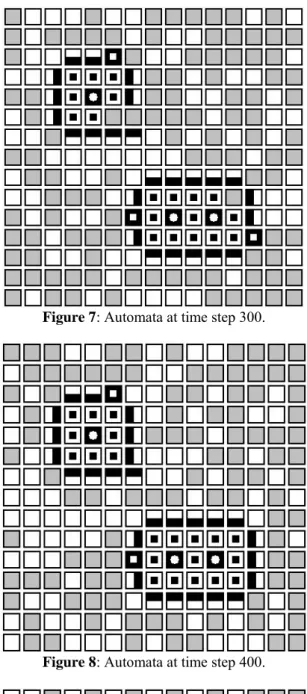
L(i,j) + E(i1,j)+E(i+1,j) E(i,j) + S(i1,j)+S(i+1,j) L(i,j) + E(i,j1)+E(i,j+1) E(i,j) + S(i,j1)+S(i,j+1) 6.3 Simulation of the Anticipatory Autopoiesis Due to the lack of space, only a single simulation will be shown, given in Figures 4, 5, 6, 7, 8 and 9.
Figure 4 gives the initial configuration of the automata system, with 90% of substrate, and 3 catalysts.
Figure 5 gives the automata systems after 100 iterative steps: a first cell membrane is created around the first catalyst, and a second cell membrane is created around the two adjacent catalysts.
Figure 4: Initial automata at time step 0
Figure 5: Automata at time step 100.
Figure 6: Automata at time step 200.
Figure 7: Automata at time step 300.
Figure 8: Automata at time step 400.
Figure 6 gives the automata systems after 200 iterative steps: the first cell membrane is almost completed, with a link that escapes the cell at the south, and the second cell membrane around the two adjacent catalysts is also almost completed with 2 lacking east and south links.
Figure 7 gives the automata systems after 300 iterative steps: the first cell membrane is almost completed, with an extra south link, and a north link that is disintegrating, and the second cell membrane around the two adjacent catalysts is completed with 2 east and west disintegrating links.
Figure 8 gives the automata systems after 400 iterative steps: the first cell membrane is completed, with an extra south link, and a north link that is disintegrating, and the second cell membrane around the two adjacent catalysts is completed with a west disintegrating link.
Figure 9 gives the automata systems after 500 iterative steps: the first cell membrane is totally completed, and the second cell membrane around the two adjacent catalysts is also totally completed, and 3 disintegrating links are also present near the two cells.
In conclusion of this simulation, we can say that the anticipatory autopoietic automata algorithm that we have developed, shows the emergence of artificial living cells, the catalysts playing the role of the genetic code and the membranes self-repair by an anticipatory autopoiesis. .
7 Conclusion
Concerning our first research question we have found that there are practically no traces of anticipation in the paper from 1974. So even if we interpret Varela's discussion of “Intentionality” in a later paper from 1991 as coming close to concept of anticipation.
Coming to the second question we have demonstrated with our computer simulations that even a very simple form of anticipation may significantly improve the effectiveness or viability of an artificial autopoietic system.
Coming to our main purpose, at last, we have found the combination of autopoiesis and anticipation being a fertile and enormously promising research field.
References
[Beer, 2004] Randall D. Beer. Autopoiesis and Cognition in the Game of Life. Artificial Life, (2004) 10:3, pp 309-326.
[Bitbol and Luisi, 2004] Michel Bitbol and Pier Luigi Luisi. Autopoiesis with or without cognition: defining life at its edge. J. R. Soc. Interface, (2004) 1, 99-107. [Bourgine and Stewart, 2004] Paul Bourgine and John
Stewart. Artificial Life, (2004) 10: 327-345.
[Collier, 2008] John Collier. Simulating autonomous anticipation: The importance of Dubois’ conjecture.
BioSystems, 91 (2008), 346-354.
[Dubois, 1997] Daniel M. Dubois, Generation of Fractals from Incursive Automata, Digital Diffusion and Wave Equation Systems, Invited Paper, BioSystems, 43, pp. 97-114, 1997.
[Dubois, 1998] Daniel M. Dubois, Hyperincursive Method for Generating Fractals in Automata Related to Diffusion and Wave Equations, Invited Paper,
International Journal of General Systems, vol. 27
(1-3), pp. 141-180, 1998.
[Dubois, 2003] Daniel M. Dubois. Mathematical foundations of discrete and functional systems with strong and weak anticipation. In Martin Butz et al. (Eds), Anticipatory Behavior in Adaptive Learning
Systems, State of the Art Survey, Lecture Notes in
Artificial Intelligence, Springer LNAI 2684, (2003) 110-132, Berlin.
[Dubois and Holmberg, 2008] Daniel M. Dubois and Stig C. Holmberg. Self-Adapting Parameters in Simulation of Management Systems. In R. Trappl (Ed),
Cybernetics and Systems 2008, Austrian Society for
Cybernetic Studies, Vienna, Vol. 1 pp 26-31.
[Holmberg, 1998] Stig C. Holmberg. Anticipatory Computing with a Spatio Temporal Fuzzy Model. In D. Dubois (Ed), Computing Anticipatory Systems, CASYS
First Int. Conference. American Institute of Physics,
Conf. Proceedings 437, 419-432, Woodbury, NY, 1998.
[Luisi, 2003] Pier Luigi Luisi. Autopoiesis: a review and a reappraisal. Naturwissenshaften (2003) 90:49-59. [Mingers et al., 1997] John Mingers and Barry McMullin.
JM’s Simple Autopoiesis Program, 1997. Program source in Pascal.
[McMullin, 1997] Barry McMullin, Computational Autopoiesis: The Original Algorithm. Working Paper: 97-01-001, Santa Fe Institute, Santa Fe, 1997.
[McMullin, 2004] Barry McMullin, 30 Years of Computational Autopoiesis: A Review. Artificial Life, Vol. 10, Issue 3, 2004.
[McMullin and Varela, 1997] Barry McMullin and Francisco J. Varela. Rediscovering Computational Autopoiesis. In Phil Husbands and Imman Harvey, editors, Proceedings of the Fourth European Conference on Artificial Life, pages 38-47, Cambridge, 1997. MIT Press.
[Rosen, 1985] Robert Rosen. Anticipatory Systems, Pergamon Press, Oxford, 1985.
[Rosen, 1991] Robert Rosen. Life Itself. Columbia University Press, New York, 1991.
[Varela, 1989] Francisco J. Varela. Autonomie et Connaissance, essai sur le vivant. Seuil, Paris, 1989. [Varela, 1996] Francisco J. Varela. The Early Days of
Autopoiesis: Heinz and Chile, Systems Research,
13(3), 407-416.
[Varela, 2000] Francisco J. Varela. Autopoiesis and a Biology of Intentionality. Paper CREA, CNRS – Ecole Polytechnique, Paris, 2000.
[Varela et al. 1974] Francisco J. Varela, Humberto R. Maturana, and R. Uribe. Autopoiesis: The Organization of Living Systems, Its Characterization and a Model.