Tien Shan Geohazards Database: Landslide susceptibility analysis
H.B. Havenith
a,⁎
, A. Torgoev
a, R. Schlögel
b, A. Braun
c, I. Torgoev
d, A. Ischuk
ea
Department of Geology, University of Liege, Liege, Belgium
b
Institut du Physique du Globe de Strasbourg, CNRS UMR 7516, Univ. de Strasbourg/EOST, Strasbourg Cedex, France
cDepartment of Engineering Geology and Hydrogeology, RWTH Aachen University, Aachen, Germany d
Institute of Geomechanics and Development of Subsoil, Academy of Sciences, Bishkek, Kyrgyzstan
e
Institute of Geology, Earthquake Engineering and Seismology, Academy of Sciences, Dushanbe, Tajikistan
a b s t r a c t
a r t i c l e i n f o
Article history: Received 27 August 2014
Received in revised form 20 January 2015 Accepted 17 March 2015 Available online xxxx Keywords: Landslide susceptibility Morphology Lithology Seismo-tectonic factors Landslide inventory verification Central Asia
This paper is the second part of a new geohazards analysis applied to a large part of the Tien Shan, Central Asia, focused on landslide susceptibility computations that are based on recently compiled geographic, geological and geomorphological data. The core data are a digital elevation model, an updated earthquake catalogue, an active fault map as well as a new landslide inventory. The most recently added digital data are a new simplified geolog-ical map, an annual precipitation map, as well as river and road network maps that were produced for the Kyrgyz and Tajik parts of the Tien Shan. On the basis of these records we determine landslide densities with respect to morphological (M), geological (G), river distance (R), precipitation (P), earthquake (E) and fault (F) distance fac-tors. Correlations were also established between scarp locations and the slope angle, distance to rivers, curvature. These correlations show that scarps tend to be located on steeper slopes, farther from rivers and on more convex terrain than the entire landslides. On the basis of the landslide density values computed for each class of the aforementioned factors, two landslide susceptibility maps are created according to the Landslide Factor analysis: thefirst one considers correlations between the landslide occurrences and the first four factors (MGRP); the sec-ond one is based on thefirst map (MGRP) combined with the seismo-tectonic influence (+E + F) on landslide distributions. From the comparison of these two maps with actual landslide distributions we infer that the dis-tances to rivers as well as to faults and past earthquakes most strongly constrain the susceptibility of slopes to landslides. We highlight several zones where the landslide susceptibilities computed for the MGRP + E + F fac-torsfit better the observed concentration of landslides than those computed for the MGRP factors alone. For a few zones, both maps produce high landslide susceptibilities that do not well reflect the observed low sub-regional landslide activity; for some cases, we consider that some influencing factors must not have been well taken into consideration, for others we show that we simply had missed landslide detections.
At the scale of the mountain range, the computed landslide susceptibility mapsfit the observed landslide distributions relatively well, but these maps only represent the spatial component of landslide hazards. Temporal aspects are not considered by this analysis.
© 2015 Elsevier B.V. All rights reserved.
1. Introduction
In this paper we present a new landslide susceptibility study applied to a large part of the Tien Shan, Central Asia. The basic inputs are a re-cently compiled landslide inventory as well as an updated earthquake catalogue and active fault map that have already been introduced in the companion paper byHavenith et al., this issue. This companion paperfirst provides a definition of the mapped ‘landslides’, considered as coherent mass movements: rockslides, rock avalanches and deep-seated slope failures marked by large displacements, mass movements in soils and soft sediments, but mostly excluding debrisflows or
singular rock falls. Second, it establishes links between the landslide and the seismo-tectonic activity on the basis of size–frequency analyses and presented case histories of earthquakes that triggered landslides in many areas of the target region. Here, this study is extended to statisti-cal spatial correlations that are also applied to other environmental fac-tors potentially influencing the regional susceptibility to slope failure.
Thefirst landslide susceptibility map covering the entire target region including the Kyrgyz and Tajik parts of the Tien Shan was presented byNadim et al. (2006). That study was part of worldwide assessment of landslide and avalanche occurrence probabilities on the basis of morphological, geological, meteorological and seismological data. As they worked at a very global scale, outputs were presented at a low resolution (kilometric or even lower). For the entire Central Asian Mountain regions, they estimate that global landslide hazard can be rated as medium to very high. They further noted that some
Geomorphology xxx (2015) xxx–xxx
⁎ Corresponding author.
E-mail address:[email protected](H.B. Havenith).
http://dx.doi.org/10.1016/j.geomorph.2015.03.019
0169-555X/© 2015 Elsevier B.V. All rights reserved.
Contents lists available atScienceDirect
Geomorphology
areas in Tajikistan are marked by the highest mortality risk due to landslides. More detailed sub-regional landslide susceptibility (LS) analyses were presented in the same period byHavenith et al. (2006a, b)for areas in the Central Tien Shan and the Maily-Say Valley, respec-tively. The evolution of landslide activity in the Maily-Say Valley over the past 50 years has been detected and analysed on the basis of pre-existing landslide maps and new analyses of aerial photographs as well as Quickbird images (Schlögel, 2009). Size–frequency analyses applied to thefive landslide inventories from 1962 to 2007 show that both the number and size of related mass movements increased. In addition, the decreasing power-law exponent over time may indicate that landslide-related hazards are increasing in the Maily-Say Valley (Schlögel et al., 2011)
Those previous studies used sub-regional inventories with 200 up to 500 mapped landslides, which are also part of the new much larger landslide inventory that represents the basis for the present susceptibil-ity analyses. The general statistical method used for our previous LS mapping was the pixel-based Landslide Factor Analysis. This one as well as other more sophisticated statistical methods (e.g. the Condition-al AnCondition-alysis based on the determination of Unique Condition Units, see Carrara et al., 1995; Clerici et al., 2002) were applied to the LS analysis within the Suusamyr Basin (Havenith et al., 2006a). Additional statisti-cal methods for LS analysis were applied to the Maily-Say Valley in a local study, such as the Information Value method, a bivariate statistical method (Yin and Yan, 1988) as well as various data mining techniques, where a multi-parameter input dataset was examined for patterns related to landslide occurrence (Braun, 2010). Related results were compared with those of a process-based (in its original form) or better analytical technique (the Newmark analysis). This latter method is commonly used to evaluate LS in seismically active regions since it was shown that in some cases such geotechnical models can successful-ly predict the regional failure potential (Jibson et al., 1998; Miles and Ho, 1999). The analysis byHavenith et al. (2006a)showed that the Newmark method produced LS valuesfitting particularly well with local landslide densities in the Suusamyr Basin if faults were considered as seismic sources. The main disadvantage of most sophisticated LS mapping methods, especially of the analytical ones is that they require a large number of inputs, including geotechnical data, which are gener-ally not available (at the required resolution) for very large areas, such as an entire mountain range. Therefore, here, only the relatively simple Landslide Factor Analysis is applied as itfits well for a LS analysis applied to a large part of the Tien Shan for which far less detailed information is available than for the smaller sub-regions. The method is based on the calculation of landslide densities within the different classes of various environmental factor maps.
The goal of the present work is not to test the performance of various LS mapping methods such as in our previous study applied to the Suusamyr Basin but to evaluate the respective contribution of different environmental factors to landslide susceptibility at the scale of a moun-tain range. Here, we define landslide susceptibility as a spatial occur-rence probability related to slope failure without considering its size of its activity in time (see, e.g.,Aleotti and Chowdhury, 1999). As indicated above, particular focus will be on the influence of seismo-tectonic factors on the regional landslide susceptibility. The main reasons for this particular focus are the high level of seismic hazard in most regions of the Tien Shan (seeAbdrakhmatov et al., 2003; Bindi et al., 2012) and the relatively frequent triggering of large landslides (N10 × 106m3) by earthquakes (Havenith and Bourdeau, 2010). During the last century, these earthquake-triggered mass movements also caused the most severe natural disasters inside or near the mountains of the Tien Shan (see e.g.Gubin, 1960; Evans et al., 2009, for the Mw = 7.4, 1949, Khait earthquake orIshihara et al., 1990, for the Mw = 5.5, 1989, Gissar earthquake). Some of them were related to consequential effects such as river damming by landslides, dam breach and downstreamfloods; a review of such effects in the Tien Shan is presented in the companion paper byHavenith et al., this issue.
2. Tien Shan Geohazards Database— inputs
For the compilation of nearly continuous datasets, for the landslide susceptibility mapping and for the production of raster information, the following geographic extent was defined (using projection of UTM 43 N, false easting 500,000): W–E — 200,000–1,000,000; S–N 4,250,000–4,850,000; thus, the target area covers 1200 × 600 km = 720 · 103km2.
The basic layer of the geohazards database is the SRTM 90 m Digital Elevation Model (DEM) that was re-sampled and interpolated at a resolution of 100 m. All other raster-image data were produced at the same 100 m resolution.
2.1. Landslide inventory, earthquake catalogue and digital active fault map The earthquake catalogue and the digital active fault map, both pro-duced by the Central Asia Seismic Risk Initiative (CASRI) project (see, e.g.,Bindi et al., 2012), cover the entire territory of Central Asia, also the areas outside the target region while a homogeneous landslide map has only been compiled within the aforementioned geographic ex-tent (Mw≥ 6.5 earthquake epicentres, active fault lines and landslides are shown inFig. 1). The landslide inventory and earthquake catalogue are presented and analysed in detail (including size–frequency statis-tics) in the companion paper byHavenith et al., this issue. The active fault map is also used as background information in that paper, but a more detailed analysis of the spatial relationship between the faults and landslides will be presented below. For these faults, maximum possible magnitudes have been estimated as well as the recurrence of such magnitudes; however, here we only consider the location of the faults and not their estimated respective activity.
Landslides were mainly digitized within Google©Earth; the digitized outlines were then reformatted as shapefile (polygon entities) for use on a common GIS platform (here, ArcGIS©10.2). This mapping had been completed only recently since for many areas high-resolution imagery was not available on Google©Earth before 2012. The entire landslide inventory includes 3462 mapped landslides: including rockslides, rock avalanches, deep-seated mass movements, loess land-slides and landland-slides in other soft soils and sediments; the outlines cover both the source and deposition (for landslide with large displace-ments) area; debrisflows and rockfalls have only been mapped if asso-ciated with large coherent mass movements. In the companion paper by Havenith et al., this issue, the landslide inventory has been subdivided into 1) a rockslide dataset (1389) and 2) a soft rock–earth slide dataset (1807); 3) a small dataset of landslides mapped outside the countries of Kyrgyzstan and Tajikistan for which the geology is not known (240); and 4) a local dataset of 26 landslides, drawn on the basis of an existing map (Gubin, 1960) of mass movements triggered by the Khait earth-quake in 1949 (26). However, for the landslide susceptibility analyses presented below, the types of landslides have not been considered (the entire inventory was used for all analyses, see landslides outlined by dark dots and polygons inFig. 1). The reason for this is that we want to determine the general effect of seismo-tectonic factors on slope stability at the scale of a mountain range disregarding the type of potential failure. Type-specific landslide susceptibility mapping is planned for sub-regions (for which more detailed geological –geotech-nical information is available) in the near future. Such an approach will also be based on separated inventories for depositional and source areas. Here, some qualitative indications of landslide type-specific susceptibility will be provided for some sub-regions, notably to outline the particular behaviour of landslides andflows in loess deposits.
For at least 100 landslides in hard and soft rocks,field observations have been collected over more than 15 years. For sub-regions, such as the Maily-Say Valley also high-resolution imagery (panchromatic and multi-spectral Quickbird) had been used to map landslides (see Schlögel et al., 2011). First mapping of landslides (before 2006) was also completed with Corona, Aster and SPOT imagery.
2.2. Geological, geographic, hydrologic and climatic data
Most of the geological, geographic (road network, location of towns and villages, and others), climatic (average annual precipitation) and hydrologic (digital map of rivers) information was provided by the Ministries of Emergency Situations of Kyrgyzstan (GIS laboratory) and Tajikistan.
For Kyrgyzstan, a fully digitized geological map was provided while for Tajikistan only a scanned geological map was available (‘Geological map of the territory of Tajikistan and neighbouring areas, scale 1:500,000, 1984’). The latter was georeferenced and only two types of formations were distinguished and digitized: hard rock (pre-Mesozoic and intrusive rocks) and soft rocks and sediments (Mesozoic, Cenozoic). The combined simplified geological map of both countries (seeFig. 1) shows that the Tien Shan is characterised by alternating, roughly East– West trending mountain ranges and intramontane basins. Palaeozoic rocks and the older basement constitute the core of the ranges (dark-coloured areas inFig. 1), whereas the basins arefilled by Cenozoic and Mesozoic sediments (light-coloured areas inFig. 1) and are mostly bordered by oppositely vergent thrust faults (Cobbold et al., 1993). The major fault structures considered as seismically active in Late Pleistocene and Holocene times (Bindi et al., 2012) are outlined in black inFig. 1.
The geohazards database also includes land-cover (grasslands, forests, and other) data that have not yet been implemented for landslide susceptibility analyses because the data were provided at a much lower (kilometric) resolution and we do not have a continuous set for the two countries of Kyrgyzstan and Tajikistan. The principal geographic information used here is the road network that may also reflect population density (a more extensive and dense network is located in populated areas).
For Tajikistan, a digital map of average annual precipitation (1984) was provided by the Institute of Geology, Earthquake Engineering and Seismology of Tajikistan. For Kyrgyzstan, only the corresponding scanned map was available (provided by the Institute of Water prob-lems and Hydropower of the National Academy of Science of the Kyrgyz
Republic). It was georeferenced and digitized and then combined with the existing digital map of Tajikistan. The compiled map of average annual precipitation covering Kyrgyzstan and Northern Tajikistan is presented together with the landslides (dots, polygons), the river net-work (light-coloured lines) and road netnet-work (dark-coloured lines) in Fig. 2. This compiled map shows that both basins at low and some basins at higher altitudes (N1500 m) surrounded by mountain ranges are marked by an arid climate (with less than 200 mm of precipitation per year). The mountain ranges are marked by a semi-arid (200– 400 mm) to humid climate (N700 mm), with largest amounts of yearly precipitation (N1000 mm) affecting high-altitude west- or northward oriented slopes (reaching 1400 mm/year) on the high western slopes of the central Fergana Range (see large blue areas in the centre of the map inFig. 2). Above 2500 m altitude most of the precipitation is recorded as snow falls.
2.3. Correlation with contributing factors
A series of environmental factors are considered for the landslide susceptibility analysis: the distance to the road network as a geographic factor; the distance to the river network and the average annual precip-itation as hydrological and climatic factors, respectively; the simplified geology and the distance to active faults as geological and seismo-tectonic factors. The four classical morphological factors, altitude, slope angle and aspect as well as curvature, have also been correlated with landslide occurrence; the influence of terrain curvature will be analysed more in detail as it may also be an indicator of the seismic influence on slope stability.Fig. 3presents the classified altitude map extracted from the 100 m SRTM digital elevation model (DEM) of the Central Tien Shan together with the hillshade that provides a rough estimate of the local relief and related morphological characteristics (steepness and orientation of slopes; location of crests and valleys influencing the curvature). In this map, digitized landslides are shown by red polygons. The thick dark lines surrounding the higher parts of most of the landslides in this region represent the outer landslide scarp limits (or‘crowns’ defined as a 300 m buffer around the scarp
Fig. 1. Simplified geological map (UTM 43N projection and geographic reference) for investigated Kyrgyz and Tajik parts of the Tien Shan (see legend for lithological subdivision – only done within the borders of both corresponding countries and the target region) on SRTM 90 m DEM (interpolated at 100 m) with overlays of earthquake data from the CASRI catalogue (250 BC until 12/2009) and USGS catalogue (01/2010–05/2014) – here only Mw ≥6.5 are presented; indicated are magnitudes larger than 6.9; the active fault map (black polylines) with thickness representing (qualitatively) the seismic activity of each fault (see location of the largest fault zone: the Talas-Fergana Fault); and landslides (dots, polygons; see legend). Borders of the Tien Shan are roughly shown by the light polygon (target region is marked by the black rectangle: 1200∗ 600 km); note, the easternmost Chinese part is not shown. ‘L’ marks the location of major lakes.
line). For the entire target region, about 1500 landslide scarps have been outlined (the map inFig. 3below shows about 1000 mapped scarps). The mapped scarp buffers were used for correlations with terrain slope and curvature as well as with the distance to rivers.
As we use the Landslide Factor analysis to compute landslide suscep-tibility,first the landslide densities have to be determined with respect to each class of the different environmental factors. For most factors, a normalised pixel-based density was calculated (Eq.1), but for the geol-ogy also the number of landslides was considered (Eq.2):
Ldp¼ ALPC ALPT APT APC ð1Þ Ldn¼ NLC NLT APT APC ð2Þ
where Ldpis the normalised pixel-based landslide density and Ldnis the normalised landslide density based on the number of landslides; ALPCis the area of landslide pixels in each class of the environmental factor map, ALPTis the total area of landslide pixels (of all landslides within the map of factor values), APCis the area of pixels in each class of the en-vironmental factor map, APTis the total area of pixels within the envi-ronmental factor map; NLCis the number of landslides in each class of the environmental factor map, NLTis the total number of landslides (within the environmental factor map). Ldpand Ldnvalues of 1 indicate
Fig. 2. Contour map of annual average precipitation on SRTM DEM interpolated at 100 m (see legend for precipitation contours) with overlays of mapped landslides (dots, polygons); rivers and lakes, road network (line symbols shown in legend).‘L’ marks the location of major lakes. The small black rectangle outlines the map shown inFig. 3.
Fig. 3. Morphology of the Central Tien Shan and North-East Fergana Basin with outlines of landslides (dots, polygons) and scarps (thick dark lines); rivers, lakes and reservoirs are shown as well as active faults (see legend). Dark arrows show typical contacts between landslides and rivers (including partial or total damming of rivers, see arrow in NW part of the map), white arrows show typical locations of scarps near mountain crests or at crest ends.
an average landslide density for a factor class; if the same values are less than 1, a landslide density below average is observed for the respective factor class while values above 1 indicate a landslide density higher than average.
The graph presenting normalised landslide pixel densities with re-spect to geology (Fig. 4a) shows that more landslide pixels are located in hard rock formations than in soft rock formations (left columns). However, the landslide number density (see middle columns in the same graph) is larger in the soft rocks than in the hard rocks. This differ-ence can be explained by the fact that hard rock landslides are generally (much) bigger than soft rock landslides andflows; thus, even though fewer landslides are located in hard rocks, the density of related pixel areas is higher for the hard rock areas than for the soft rock areas. It should be noticed that in this case the (likely) limited completeness of the landslide inventory for smaller landslides (many areas in the Tien Shan are only covered by 5 or 10 m resolution SPOT imagery in Google© Earth) might be one reason for this paradoxically lower landslide densi-ty in soft rocks; we consider that most of the‘undetected’ smaller (≪105m3) landslides are located in soft rocks (see also discussion on landslide inventory completeness in the companion paper by Havenith et al., this issue). Further, if we exclude zones with slopes smaller than 5° (generally present in the wideflat areas covered by soft sediments outside the mountain range) from the correlation, we can notice that a slightly higher density of landslide pixels can be ob-served in soft rock areas than in hard rock areas (green columns). This is due to the fact that the number of pixels in soft rocks is much lower, as almost half of soft-rock pixels are located in zones with slopes smaller than 5°, while less than 10% of the hard rock pixels are located in these gently dipping orflat areas. Therefore, the ratio of landslide pixel areas per geology class pixels increases for soft rock landslides and compara-tively decreases for hard rock landslides. For the landslide susceptibility analysis we considered these latter densities of landslide pixel areas in each geological class (soft rocks have a slightly higher susceptibility to slope instability than hard rocks, respectively marked by values of
1.13 and 0.95). It can be noticed that previous studies byHavenith et al. (2006a,b)showed similarly higher susceptibility of soft rocks to landsliding within two sub-regions of the target area (Suusamyr region and Maily-Say Valley, marked by arrows‘Suu’ and ‘M-S’ inFig. 4a, respectively). There, it could partly be proved that the lower shear resistance of the materials is responsible for the higher susceptibility to slope failure.
As a climatic factor influencing slope stability we consider the map of average annual precipitation that was compiled from various sources (see above inFig. 2). The variations in landslide density with respect to the distribution of average annual precipitation (in mm) are present-ed inFig. 4b. The morphological parameter most strongly influencing precipitation is the altitude. Related correlations (also shown in Fig. 4b) as well as those based on precipitation show that most land-slides are located in mid to high altitude zones (1400–2400 m) marked by medium high precipitations (400–700 mm per year). From this graph we can also see that fewer landslides are located at the highest altitudes marked by maximum precipitation— this aspect will be discussed in the next section as it concerns also the validity of the land-slide inventory for high mountain areas. The lower concentration of landslides in areas marked by lower precipitation seems to be obvious, but also here indirect effects have to be taken into account: especially zones marked by very low precipitation are located at the bottom of mountain basins orflat lowlands and, for this specific morphological reason, are less susceptible to slope instability. From these observations we infer that the landslide density — precipitation correlation is relatively weak (also due to the likely low resolution of initial rain gauge data used to produce the precipitation map) while the influence of altitude on landslide density is clearly stronger.
The graph inFig. 4c shows correlations between landslide location and their distance to roads and rivers. It can be seen that most landslides are located near rivers and similarly also close to roads (note the almost overlapping red and blue lines). The fact that landslides (and especially associated deposits) are located close to rivers is almost obvious as
Fig. 4. Graphs of normalised landslide densities with respect to various factors: simplified geology (a: soft and hard rock) over Kyrgyzstan and Tajikistan, (pixel-based and number-based, considering also only slopesN5°); the altitude and average annual precipitation (b); the distance to roads and rivers, also the distance of landslide scarps to rivers is shown (c); slope angle for landslides and scarps (d); slope orientation (aspect) considering all slopesN5° (note, class 0 stays for flat areas); e) (total) and curvature (f). In f) also the density of 1500 mapped landslide scarps with respect to curvature is presented. Curvature was calculated for the 100 m SRTM DEM and the same DEM interpolated at 250 m resolution (see legend for correspond-ing lines 1, 2, 3). The arrows‘Suu’ and ‘M-S’ show the classes where the highest landslide density values had been obtained, respectively, for the Suusamyr sub-region (byHavenith et al., 2006a) and for the Maily-Say Valley (byHavenith et al., 2006b).
landslide material typically moves down to the valley bottom where the rivers are located, but this graph also shows that river erosion must be considered as an important trigger factor. For several large landslides we actually know that they were activated by river erosion. A famous example is the Ayni rockslide that occurred in 1964 along the Zeravshan River (see companion paper byHavenith et al., this issue). However, we also identified source zones (scarps) of many large landslides that were most likely not in contact with any river when the mass movement was activated (see also maximum density of scarp zones at more than 1000 m away from the river inFig. 4c (curve 3). Most of these mass movements reached the nearest river due to the large runout (examples are shown in the companion paper byHavenith et al., this issue). The similar proximity of landslides to roads can again be explained by an indirect effect: most roads were built near the rivers along the valley bottoms (where landslide distal zones are often present), because this flat terrain is better for road construction and transport. Actually, we consider that the influence of roads on large slope failures can be con-sidered as very limited while their construction certainly contributes to minor (b105m3) slope instabilities. In this regard, it should be noted that many large landslides were triggered in pre-historic times when there were no roads.
The correlations between landslide location and the morphological factors, slope angle, slope orientation and curvature are presented in the graphs d), e) and f) inFig. 4. The twofirst graphs show that land-slides are preferentially located on slopes with an angle of 15–25° and oriented towards the North-West. The correlation with slope angles is clearly stronger (maximum density of entire landslides of 1.7 for slopes of 15°) than the one with slope orientation (maximum density of 1.2 on NW slopes). The high density of landslides in areas marked by relatively gentle slopes (b20°) can be explained by the fact that at least part of the landslide material (now the landslide deposits) had moved to lower more gently sloping areas while the source region is generally marked by larger slope angles (see curve 2 in the graph 4d with maximum of scarp density for slopes of about 40°). It should be noted that the obser-vation of the weak influence of slope orientation on landslide suscepti-bility at the scale of the entire Tien Shan shown inFig. 4e is only partly supported by previous landslide susceptibility studies completed in the aforementioned Suusamyr and Maily-Say regions (Havenith et al., 2006a,b), where densities of landslides (especially in soft rocks and sed-iments) are clearly higher (~1.5) on NW-N oriented slopes. This locally clear effect of slope orientation on landslide susceptibility is smoother if a large part of the Tien Shan is considered probably due to the different orientations of geological structures (and other changing conditions, such as precipitation distribution) over such large areas.
Finally, we present also spatial correlations between the presence of landslides (and associated deposits) and slope curvature (see curve 1 in the graph 4f). The same correlations were also done for scarps of some 1500 large landslides that were mapped (as polylines) all over the Tien Shan (they are shown for a sub-region inFig. 3). Scarp locations were analysed with respect to curvature for the DEM resampled and in-terpolated at 100 m (curve 2 in graph 4f) and with respect to a map of curvature computed on the basis of a DEM resampled and interpolated at 250 m (curve 3 in graph 4f). The 250 m DEM was added to the initial one in order to compute curvature over larger areas and thus to assess the influence of ‘lower frequency’ topography changes on scarp distri-butions. The first correlation between landslide (and associated deposits) location and curvature (for 100 m resolution DEM) shows a slightly larger concentration of mass movement pixels in areas marked by concave surface curvature. However, the landslide scarps are prefer-entially located on convex slopes. This effect is stronger for the curva-ture computed from the 250 m DEM than from the 100 m DEM. The difference between total landslide density and scarp density over the curvature map can be explained by the fact that large parts of most land-slides (belonging to the deposits) moved to areas near the valley bottom (see also correlation with rivers) clearly marked by concave curvature, while the scarps or source areas formed higher on slopes presenting a
convex curvature. We already discussed this difference inHavenith et al. (2006a)where we presented a more detailed landslide suscepti-bility analysis for the Suusamyr Basin. It should be noted that the convex morphology near scarps is partly due to the scarp itself as it represents a local convex slope break (of variable size according to the size of the landslide and the intensity of failure). However, this convex morpholo-gy affects only the inner (within the landslide) part of the 300 m buffer. The other part of the 300 m buffer is outside the landslide and thus only affected by the natural slope morphology (and not by the specific scarp morphology). The influence of the general convex curvature of larger parts of the mountains on the location of landslide source areas (the scarps), is better highlighted by correlations between scarps and the curvature map computed on the basis of a lower 250 m resolution DEM. The curvature of each pixel thus represents the morphology of an area with a diameter of at least the double of the pixel size (i.e., 500 m, as the curvature represents the double derivative of the surface). We consider that only a few scarps of very large landslides can induce significant curvature over such an extent; for 90% of the landslides at least, the curvature computed over this area should repre-sent the one of the natural slope. A more detailed discussion on this par-ticular morphological influence on slope stability is presented below. 2.4. Comments on particular correlation results
First, we would like to outline possible reasons for the lower land-slide density at higher altitudes marked by larger precipitation rates. On one hand, it could be that not all landslides have been identified at higher altitudes (above 2500 m)– especially deep-seated rockslides marked by small displacements or singular rock falls– as not all these areas are covered by high-resolution imagery in Google©Earth (see alsoHavenith et al., this issue, for more detail on this aspect); further, we tried to avoid mapping deposits looking similar to moraines (especially where recognition is hampered due to low image resolu-tion). Actually, on older maps from Soviet times many rock avalanche deposits are indicated as moraines as the source area of these mass movements are sometimes located at great distances (N5 km) from the deposits. On the other hand, the lower landslide susceptibility at higher altitudes can partly be explained by the fact that these areas are often made of stronger rocks, resistant to erosion; further, perma-frost contributes to slope stability above altitudes of 3000–3500 m (for most of the Tien Shan). This confirms that no direct link can be established between average annual rainfall distribution and landslide activity if statistics are applied to all the landslides covering the entire territory of the Tien Shan. However, we also know that some specific types of landslides in some sub-regions covered by thick loess deposits, such as earth slides andflows, are preferentially triggered by intense and long lasting rainfall. To outline this dependence of landslide occur-rence on precipitation, sub-regional and landslide type-specific correla-tions would be needed. Such type-specific and sub-regional landslide analysis would also better show the influence of slope orientation on slope stability. For instance, the more‘climatic’ Loess flows are clearly distributed within clusters that are not only related to loess cover thick-ness but also to the wetthick-ness of soils that is generally larger on north-and north-westward oriented slopes.
Further, the temporal component needs to be considered; e.g.,Havenith et al. (2006b)clearly showed that the activation of soft rock landslides in the Maily-Say Valley is strongly influenced by season-al variations of rainfseason-all and snowmelt. Yet, the effect of rainfseason-all on the stability of large rock slopes cannot be easily shown as these slopes gen-erally respond to long-term climatic changes. For some types of giant rockslides we consider that their triggering is much more controlled by structural and seismo-tectonic factors than by climatic ones (even if we consider different climatic conditions in the past). The structural factor cannot be analysed here as we have only very local information on rock structures, while the tectonic factor can be analysed using the active fault maps (see analysis related toFig. 6below). In this regard,
it is interesting to notice that the source area of the largest rockslide of the Tien Shan, Beshkiol, in Naryn Valley (see red polygon in SE corner of the map inFig. 3), located in a relatively arid zone is bounded by a series of faults.
Second, it is important to know that some correlations shown above do not only mark landslide susceptibility with respect to a specific envi-ronmental factor, but also provide information on the exposure of spe-cific locations or elements to landslide impacts. For instance, the graph inFig. 4c, highlights the exposure of rivers and roads to landslide im-pacts. Actually, roads probably belong to the constructed objects that are most frequently impacted by landslides in mountain regions. The exposure of rivers to landslide impacts can even be more important for landslide risk analyses as it is at the origin of new types of induced hazard: the formation of (partial or full) blockages, upstreamflooding with possible destabilisation of slopes around the new lake, down-streamflooding after (partial or total) dam breach, formation of related debrisflows — examples of all these hazards are presented in the companion paper byHavenith et al. (this issue).
Finally, we add one comment concerning the clearly stronger concentration of scarps on convex slopes (especially with respect to curvature computed for a lower resolution 250 m DEM— compared to the initial interpolated 100 m DEM) while landslide material is prefer-entially located in concave areas. As already highlighted byHavenith et al. (2003andHavenith et al., 2006a), this preferential initiation of slope failure near convex morphologies, such as mountain or hill crests, convex slope breaks, borders of canyons and terraces, might be the signature of the seismic influence on slope stability. This signature seems to be particularly strong in the Tien Shan (and even predominant compared to climatic or hydrologic effects if large rock slope failures are considered). Also for other seismic regions and areas hit by known earthquakes, it was shown that landslide scarps are preferentially locat-ed near hilltops and convex slope breaks (see, e.g.,Harp et al., 1981, for Guatemala andDurville and Méneroud, 1982, for Northern Algeria, among many others). This is due to the fact that the seismic ground mo-tion can be strongly amplified over convex ground surface due to wave focusing effects (induced both by the geometry itself and by the often more strongly weathered rocks forming the convex morphologies). Examples of clear links between landslide occurrence and earthquake ground motion in the Tien Shan are presented in the companion paper byHavenith et al. (this issue).
2.5. Landslide susceptibility mapping
On the basis of the previous correlations, a landslide susceptibility map was computed according to the Landslide Factor method. The first step involved the creation of landslide density maps for the differ-ent environmdiffer-ental factors: therefore, the landslide density values shown inFig. 4were attributed to the corresponding classes of each en-vironmental factor map. Then, various landslide density maps were multiplied with each other to obtain a landslide susceptibility map. For thefirst landslide susceptibility map ‘MGRP’ (for morphology, geol-ogy, river, precipitation), the landslide density maps computed for slope angle (here the scarp density was used for the part of the inventory where deposits could be separated from source areas to show the re-spective distribution over slopes) were multiplied with those based on slope orientation, curvature (scarp density for 100 m DEM curvature was used), altitude, geology (here the density computed for slopes N5° was used), distance to rivers and average annual precipitation. The precipitation factor was preferred to the altitude factor as we consider the latter as an indirect trigger (below the permafrost area) while precipitation may directly influence slope stability. The final multiplication product map presented inFig. 5shows susceptibility classes corresponding to intervals of multiplied density values. Five sus-ceptibility classes were defined: lowest, low, medium, high and highest. Lowest susceptibility was defined for multiplied density values of less than 0.1 while highest susceptibility was defined for resulting values
or more than 10, smaller intervals were defined for low susceptibilities and bigger ones for large susceptibilities. If we compare thefinal distri-bution of landslide susceptibility (LS) values with the actual landslide distribution, we can notice that zones marked by higher landslide con-centration are generally also highlighted by increased susceptibility; most of these high to highest susceptibility zones are located along riv-ers (see greenish areas marking high susceptibility along rivriv-ers plotted on the map inFig. 5). Thefit is best where landslides are preferentially located in narrow valleys with steep valleyflanks. This can be related to the high density values obtained for the landslide occurrence– distance to rivers correlation (densityN 2 near rivers) that contributes most to the multiplication product. As discussed above, this is not nec-essarily related to a strong contribution of river erosion to slope instabil-ity but is partly depending on indirect factors, such as the steeper slopes located near rivers and the accumulation of landslide material (the deposits) near the valley bottom (even if the initial failure is located relatively far from it). However, we can also outline some problematic zones (see black ellipses inFig. 5) where the LS either over- or underes-timates observed landslide density. For instance, in the Suusamyr Basin (zone 1 inFig. 5), the computed low LS does not reflect the higher con-centration of landslides. The same can be observed for zones 5 and 6 near the south-eastern border of the Fergana Basin while in zones 2, 3, 4, 7 and 8 the computations seem to overestimate the actual sub-regional landslide susceptibility (few landslides were detected in those areas).
Below it will be discussed if the relatively weak concentration of land-slides in those 4 areas (and other smaller not highlighted zones) is due to missed landslide detections or due to some additional factors influencing landslide susceptibility that were not considered for this map. The latter could also explain why landslide susceptibility has apparently been underestimated in the zones 1, 5 and 6.
Therefore, landslide susceptibility has also been computed by taking into account the seismo-tectonic factors introduced above: the earth-quake catalogue and the map of active faults. First, two separate maps of distances, respectively, to Mw≥ 6.5 earthquake epicentres and to faults were computed. For the latter, we considered both, the large active fault map that was produced for all Central Asia (CASRI) and sub-regional fault maps created for the Central Tien Shan. A single dis-tance map was created by computing the square root of the multiplied distances to, respectively, earthquakes and faults.
This resulting map presented inFig. 6shows light-coloured zones near past earthquakes and faults and dark-coloured areas far from earthquakes and faults. Landslide densities were calculated with respect to the initial‘distance to Mw ≥ 6.5’, ‘distance to fault map’ (CASRI fault map), to the‘distance to all faults’ (including the CASRI and the sub-regional Central Tien Shan map). Related correlations are compared to the landslide density–distance to rivers map in the graph shown in lower right corner ofFig. 6. The correlations between landslide locations and distances to faults/earthquake epicentres all show a higher land-slide density near these seismo-tectonic elements. However, compared to the correlation with the landslide density–distance to rivers map, the distribution of landslides is spatially less constrained with respect to the seismo-tectonic elements. This is likely to be related to the wider spatial influence of major fault structures and large earthquakes on slope sta-bility (connected with the dip of faults, most of which are thrust faults with earthquake epicentre locations often far from the fault outcrop, but some large faults also have an important if not predominant strike-slip component as well as the depth of earthquake hypocentres). The same graph inFig. 6also shows the landslide densities with respect to the combined distance to earthquake and fault map (curve 4 in the graph in the lower right corner). A series of white arrows plotted on the map inFig. 6highlight the presence of landslide clusters near faults or past earthquake epicentres. The most prominent example is the high concentration of landslides in the epicentral area of the Mw = 7.4 Khait earthquake that occurred in 1949 in Northern Tajikistan (highlighted in Fig. 6).
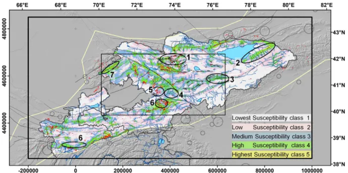
As for the other environmental factor maps, landslide densities com-puted with respect to the combined distances to faults and Mw≥ 6.5 earthquake epicentres werefirst attributed to corresponding distance classes. The resulting landslide density map was then multiplied with the MGRP landslide susceptibility map. The resulting‘MGRP + E + F’ landslide susceptibility map (MGRP defined above combined with earthquakes‘E’ and faults ‘F’) is presented inFig. 7. For this map, the samefive susceptibility classes as for the MGRP map were defined: low-est, low, medium, high and highest susceptibility. However, in the MGRP + E + F LS map, the lowest susceptibility class corresponds to
multiplied landslide density values of less than 0.05 (0.1 for the MGRP LS map) and highest to values of 15 (10 in the MGRP LS map) mainly in order to obtain classes of a size similar to the one used in the MGRP LS map.
3. Discussion: performance of susceptibility mapping
First, we can qualitatively compare the MGR + E + F LS map with the MGRP LS map by calculating the difference between the two maps. To analyse such differences we zoom in on the Central Tien
Fig. 5. Landslide susceptibility map (see 5 classes of LS) considering MGRP, morphological (M = slope angle, aspect, curvature, altitude), geological (G), hydrological (R = distance to rivers), climatic (P = average annual precipitation) factors. Black ellipses outline zones where the MGRP susceptibility map either significantly over- or underestimates the observed landslide density.
Fig. 6. Combined fault (see black lines)— Mw ≥ 6.5 earthquake (circles, note for most large earthquakes an hypocentral depth of 10 km is adopted according to available seismological data) distance map (see text for explanation), colours indicating distances from 4 km (light) to more than 40 km (dark). Landslides are outlined by dark dots, polygons. White arrows indicate the presence of landslide clusters near faults or past earthquake epicentres. Lower right corner: graph of landslide densities for distances to rivers (curve 1), all faults (curve 3), Mw≥ 6.5 earthquake epicentres (curve 2), and (curve 4) for the combined distances to earthquakes (E) and faults (F) as shown by the map in this figure.
Shan and Eastern Fergana region (Fig. 8) where some problematic zones had been outlined on the MGRP LS map (see ellipses inFig. 5plotted also on the MGRP + E + F LS map inFig. 7). Positive differences (MGRP + E + F LS N MGRP LS) and negative differences (MGRP + E + Fb MGRP) are highlighted in the map inFig. 8, respec-tively, by violet and by brown areas; zones marked by similar LS values are marked in beige. As could be expected, the MGRP + E + F LS map shows higher landslide susceptibility values along fault zones and near epicentres of past Mw≥ 6.5 earthquakes. Therefore, now much larger LS values were obtained along the faulted border of the Suusamyr Basin (zone 1) and the regions in the south of it, which better reflects the large concentration of landslides in this area (compared to the
corresponding MGRP LS map). The same can be observed for zone 6 and partly also for zone 5 near the South-Eastern border of the Fergana Basin. In contrast, in zone 4 the LS values were reduced by adding the seismo-tectonic factors to the susceptibility computations (compared to the previous MGRP LS map). This reductionfits well with the lower landslide concentration in this area— which can therefore be related to the greater distances from past earthquake epicentres and major faults. However, in the two other problematic zones 3 and 7 outlined in the map inFig. 8, the additional seismo-tectonic component did ap-parently not improve thefit between landslide susceptibility assess-ment and known landslide concentration: LS values were increased compared to the MGRP LS map, while only a few landslides were
Fig. 7. Landslide susceptibility map MGRP + E + F considering morphological, geological, hydrological, climatic, as well as seismo-tectonic (combined distance to epicentres of Mw≥ 6.5 earthquakes‘E’ shown by circles and to active faults ‘F’ shown by black lines in the map) factors. Landslides are outlined in red. Black ellipses outline zones where the MGRP susceptibility map either significantly over- or underestimates the observed landslide density. The rectangle delimits the map inFig. 8showing the result of subtraction of the MGRP map from the MGRP + E + F map.
Fig. 8. Map of differences between the MGRP and the MGRP + E + F landslide susceptibility maps (here, only shown for Central Tien Shan and Fergana Basin). Zones presenting larger MGRP compared to MGRP + E + F landslide susceptibility are marked by‘b’ sign. Landslides marked by light dots were detected in areas after the susceptibility calculations where related maps either over- or underestimated observed landslide density (based on initially identified landslides shown by dark dots, polygons).
detected in these zones. Also, along the Talas-Fergana Fault (see loca-tion inFig. 3), crossing obliquely the Tien Shan from SE to NW, the in-creased LS (reaching maximum values in some areas along the fault) does not wellfit the medium concentration of landslides in that area. To explain these discrepancies wefirst checked if some landslide occur-rences might not have been missed in these zones (the check was also performed for zones 2 and 8 not shown inFig. 8but marked onFigs. 5 and 7). Landslides detected through this verification are outlined in yellow inFig. 8. First, we verified the completeness of our landslide in-ventory in zones 2 and 3. There, we met two problems (already outlined byHavenith et al., this issue): the zones are not entirely covered by high-resolution imagery and many areas are located at higher altitudes where we could not clearly distinguish landslide from moraine material (considering the available image quality). Nevertheless, some addition-al clear landslides could be detected (see yellow dots in zone 3)— but these new detections do not significantly increase the previously observed landslide concentration. Thus, here we consider that both LS maps still overestimate the known landslide activity probably because the rocks are particularly strong in these areas. For zone 4, also a few additional slope failures were detected, but the concentration of landslides is still small compared to the neighbouring zones. Thus, the larger distance of this zone to past earthquakes and major faults might be the cause of the reduced slope instability there. Most addition-al landslides (about 35 newly mapped landslides) were detected in zone 7 in the western Tien Shan (see concentration of yellow outlines in zone 7 inFig. 8), where the previous mapping of landslides was obvi-ously incomplete. All the newly detected landslides are located along the NE–SW oriented fault crossing this zone, which fits well with the in-creased LS represented by the MGRP + E + F map (highest LS class) compared to the slightly lower LS of the MGRP map (high LS class). It should also be noted that additional landslides were detected along the Talas-Fergana fault (see yellow outlines in the middle of the map inFig. 8). With these additional landslides, we now observe a medium to high landslide concentration almost all along the Talas-Fergana Fault (besides for the SE segment located at altitudes higher than 2500 m where no landslides had been detected).
If we compare LS shown for zone 8 (north of Dushanbe, Tajikistan) by the MGRP + E + F map with the one indicated by the MGRP map, we can see that it is strongly reduced if the seismo-tectonic factors are considered. Thus, here the larger distance to major faults and past earthquakes could also explain the weaker landslide activity observed in this zone (also after checking, no additional landslides were found in this area).
It should be noted that after the experience of incomplete landslide recording in some zones the whole area was checked again and no additional large slope failures had been found. Thus, now we are quite confident that at lower altitudes (b2500 m) all rock avalanches and massive rockslides as well as soft sediment slides larger than 5 · 104m2have been mapped.
Finally, we assess statistically the quality of the two LS maps (MGRP and MGRP + E + F). The analysis is summarized by the graph inFig. 9. The columns show both the scarp and landslide densities obtained for the different susceptibility classes both for the MGRP and the MGRP + E + F LS map. From the column graph, it can be seen that the highest susceptibility class of the MGRP + E + F map contains five times more landslides than average (about 3 times more for the MGRP map). Thus, we can note that the performance of the MGRP + E + F LS map is clearly higher than the one of the MGRP LS map. The general graph also shows the size of the susceptibility classes (in terms of percentage of the entire map: curve 1 for the MGRP LS map, curve 2 for the MGRP + E + F map) and the percentage of landslides contained in it (curve 3 for MGRP map, curve 4 for the MGRP + E + F map). If we combine all these graphs, it can be seen that the maximum density of landslides in the highest LS class is due to the small size of the LS class and the relatively large number of landslides. However, the total surface area of landslides is largest for the high LS class (the medium LS class for the MGRP map) because these LS classes are much larger. Therefore, we consider the landslide density in the highest LS class as ‘specifically high’ and the one of the high LS class as ‘generally high’. The landslide density of the other classes is average (around 1) for the medium class and low (0.3b LS b0.7) and lowest (b0.2) for the low and lowest LS class, respectively.
The performance of the maps indicated above cannot directly be considered as prediction potential as we did not divide the landslide inventory into a‘training set’ and ‘validation set’. Only landslides not considered for the LS mapping (the‘validation set’) and for which the fit with computed LS (based on the ‘training set’) can be tested may be used to assess this prediction potential (Chung and Fabbri, 1999). However, from a LS study performed over such a large extent (almost covering an entire mountain range) we may at least infer that especially the MGRP + E + F LS map reproduces well the trend of the observed landslide activity (besides for zones 2 and 3 where most likely specific lithological or structural aspects were not well taken into account). Further, the landslides detected in zone 7 after completion of the LS computations may be considered as a small‘validation set’ for this specific zone that confirms the high LS computed there.
Fig. 9. Graphical analysis of susceptibility computation results showing landslide and scarp densities (filled and white columns, resp.) for each of the 5 susceptibility classes (low to high) computed for the MGRP (columns S1, S2) and the MGRP + E + F (columns S3, S4) susceptibility maps. Percentage of landslide areas per susceptibility class (compared to all landslide areas) and of susceptibility class compared to the sum of all classes are shown by curves 1 and 3 for MGRP and curves 2 and 4 for MGRP + E + F susceptibility classes; curves 1 and 2 indicating susceptibility class %; curves 3 and 4 indicating landslide class %.
4. Conclusions
In this paper we analysed landslide susceptibility for a large part (1200∗ 600 km) of the Tien Shan, Central Asia. This study is based on a new landslide inventory and a recently compiled set of hazard-relevant morphological, geological, climatic–hydrologic and seismo-tectonic information. Landslide susceptibility was analysed with respect to the aforementioned factors using the Landslide Factor analysis. The correlations between landslide occurrences and the various factors show that the distances to rivers as well as to faults and past earth-quakes most strongly constrain the susceptibility of slopes to landslides. For a series of zones, it could be observed that the landslide susceptibil-ity computed by considering the additional seismo-tectonic factorsfits better the observed concentration of landslides than those computed for the other factors alone. Here, it should be noted that only the short-distance spatial relationship between landslide location and earthquake epicentres and fault lines (outcrops) was analysed in this paper. There are also a series of examples of remote effects of earth-quakes on slope failure activation that were not considered here. The strongest remote effects are known for several deep focal MwN 6.5 earthquakes in the Hindu Kush and Pamir that caused extensive activa-tion of monitored landslides in the Angren mining region, Uzbekistan (Niyazov and Nurtaev, 2014), in former mining in Kyrgyzstan (Torgoev et al., 2013) and near the Baipaza Hydropower station in Tajikistan (Havenith et al., 2013), at distances of more than 200 km up to 700 km from the hypocentre. One reason for the triggering of various observed geomechanical processes could be related to the particularly low frequency shaking induced earthquakes at those distant sites. However, more detailed investigations and numerical simulations are required to understand these phenomena and to incorporate them into a coupled earthquake-landslide hazard assessment.
Further, within a few areas, the computed landslide susceptibility maps clearly overestimate the observed low sub-regional landslide activity; for two zones in the eastern part of the target region, several reasons may explain the lower landslide density observed there (compared to the one that could be expected according to the landslide susceptibility map):first, these higher mountain (remote) areas are not entirely covered by high-resolution imagery in Google©Earth; thus, smaller mass movements could not be identified; second, increased slope stability there could be caused by particular (yet, at present, un-known) lithological-structural factors— but this can only be confirmed afterfield visits or by using a more detailed geological map combined with higher resolution remote imagery. For two others in the Central and Western Tien Shan, we show that actually not all landslides had been mapped. After adding these landslides, a higher landslide concentration can be observed that is again bestfit by the landslide susceptibility map additionally implementing correlations with the seismo-tectonic factors because most newly detected landslides are located along fault zones. But, why did we mention the problem of undercounting of landslides in those small regions, while we might as well have hidden this aspect? Actually, we wanted to show that landslide susceptibility mapping might help assessing the validity of the existing landslide inventory, especially in remote areas. At present, we are applying a similar stepwise approach to landslide recording– susceptibility mapping under similar (and even less favourable— due to dense vegetation) conditions along the Western Branch of the East African Rift where the landslide inventory controls the susceptibility mapping and vice versa. The next step is to subdivide the complete inventory into landslide types, distinguishing between source and de-positional areas and to produce type-specific susceptibility. Therefore, we would adopt a method similar to the one used byHermanns et al. (2012). Notwithstanding the goodfit between computed landslide susceptibility maps and observed landslide distributions, the limits of landslide susceptibility assessment need to be clearly outlined: the presented maps only give a partial estimate of landslide hazards. They do not provide any indication on the important temporal landslide
hazard component (including occurrence in time and recurrence of events) and on possible coupled hazards such a river damming by landslides, dam breaches and related lake outbursts.
Acknowledgements
Part of this study has been supported by the NATO Science for Peace Project (983289)‘Prevention of landslide dam disasters in the Tien Shan, LADATSHA’, 2009–2012. We thank the The State Agency on Geol-ogy and Mineral Resources of the Kyrgyz Republic (Zhukov Yu. V.) as well as the Ministries of Emergency Situation of the countries of Kyrgyzstan and Tajikistan for providing inputs for the digital geological map. We are also grateful to the Institute of Water Problems and Hydro-power of the National Academy of Science of the Kyrgyz Republic (Kuzmichenok V. A.) for having provided the basic map allowing us to produce the digital average annual precipitation map of Kyrgyzstan.
References
Abdrakhmatov, K.Ye., Havenith, H.-B., Delvaux, D., Jongmans, D., Trefois, P., 2003. Proba-bilistic PGA and Arias Intensity maps of Kyrgyzstan (Central Asia). J. Seismol. 7, 203–220.
Aleotti, P., Chowdhury, R., 1999.Landslide hazard assessment: summary review and new perspectives. Bull. Eng. Geol. Environ. 58, 21–44.
Bindi, D., Abdrakhmatov, K.Ye., Parolai, S., Mucciarelli, M., Grunthal, G., Ischuk, A., 2012.
Seismic hazard assessment in Central Asia: outcomes from a site approach. Soil Dyn. Earthq. Eng. 37, 84–91.
Braun, A., 2010.Investigation of landslide susceptibility in Maily-Say, Kyrgyzstan, with data mining methods. Master's Thesis, Georesources Management. RWTH Aachen, Germany (131 pp.).
Carrara, A., Cardinali, M., Guzzetti, F., Reichenbach, P., 1995.GIS technology in mapping landslide hazard. In: Carrara, A., Guzzetti, F. (Eds.), Geographical Information Systems in assessing natural hazards. Kluwer Academic Press, Dordrecht, The Netherlands, pp. 135–175.
Chung, C.F., Fabbri, A., 1999.Probabilistic prediction models for landslide hazard mapping. Photogramm. Eng. Remote Sens. 65, 1389–1399.
Clerici, A., Perego, S., Tellini, C., Vescovi, P., 2002.A procedure for landslide susceptibility zonation by the conditional analysis method. Geomorphology 48, 349–364.
Cobbold, P.R., Davy, P., Gapais, D., Rossello, E.A., Sadybakasov, E., Thomas, J.C., Tondji Biyo, J.J., de Urreiztieta, M., 1993.Sedimentary basins and crustal thickening. Sediment. Geol. 86, 77–89.
Durville, J.L., Méneroud, J.P., 1982.Phénomènes géomorphologiques induits par le séisme d'El Asnam, Algérie. Comparaison avec le séisme de Campanie, Italie. Bull. liaison Labo. P. et Ch. 120, 13–23 (in French).
Evans, S., Roberts, N., Ischuk, A., Delaney, K.B., Morozova, G.S., Tutubalina, O., 2009. Land-slides triggered by the 1949 Khait Earthquake, Tajikistan, and associated loss of life. Eng. Geol. 109, 195–212.
Gubin, I.E., 1960.Patterns of seismic manifestations of the Tajikistan territory (geology and seismicity). Academy of Sciences of USSR Publishing House, Moscow (464 pp., (in Russian)).
Harp, E.L., Wilson, R.C., Wieczorek, G.F., 1981.Landslides from the February 4, 1976, Guatemala Earthquake. USGS, Washington (44 pp.).
Havenith, H.B., Bourdeau, C., 2010.Earthquake-induced hazards in mountain regions: a review of case histories from Central Asia— an inaugural lecture to the society. Geol. Belg. 13, 135–150.
Havenith, H.B., Strom, A., Jongmans, D., Abdrakhmatov, K., Delvaux, D., Tréfois, P., 2003.
Seismic triggering of landslides, Part A:field evidence from the Northern Tien Shan. Nat. Hazards Earth Syst. Sci. 3, 135–149.
Havenith, H.B., Strom, A., Cacerez, F., Pirard, E., 2006a.Analysis of landslide susceptibility in the Suusamyr region, Tien Shan: statistical and geotechnical approach. Landslides 3, 39–50.
Havenith, H.B., Torgoev, I., Meleshko, A., Alioshin, Y., Torgoev, A., Danneels, G., 2006b.
Landslides in the Mailuu-Suu Valley, Kyrgyzstan— hazards and impacts. Landslides 3, 137–147.
Havenith, H.B., Abdrakhmatov, K., Torgoev, I., Ischuk, A., Strom, A., Bystrický, E., Cipciar, A., 2013.Earthquakes, landslides, dams and reservoirs in the Tien Shan, Central Asia. In: Margottini, C., Canuti, P., Sassa, K. (Eds.), Landslide Science and Practice. 6. Springer Verlag, Berlin Heidelberg, pp. 27–31.
Havenith, H.-B., Strom, A., Torgoev, I., Torgoev, A., Lamair, L., Ischuk, A., Abdrakhm atov, K., 2015.Tien Shan Geohazards Database: earthquakes and landslides. Geomorphology, Special Issue‘Geohazards Databases’ (this issue).
Hermanns, R.L., Hansen, L., Sletten, K., Böhme, M., Bunkholt, H.S.S., Dehls, J.F., Eilertsen, R.S., Fischer, L., L'heureux, J.S., Høgaas, F., Nordahl, B., Oppikofer, T., Rubensdotter, L., Solberg, I.-L., Stalsberg, K., Yugsi Molina, F.X., 2012.Systematic geological mapping for landslide understanding in the Norwegian context. In: Eberhardt, E., Froese, C., Turner, A.K., Leroueil, S. (Eds.), Landslides and engineered slopes: protecting society through improved understanding. Taylor & Francis Group, London, pp. 265–271.
Ishihara, K., Okusa, S., Oyagi, N., Ischuk, A., 1990.Liquefaction-inducedflow slide in the collapsible loess deposit in Soviet Tajik. Soils Found. 30, 73–89.
Jibson, R.W., Harp, E.L., Michael, J.A., 1998.A method for producing digital probabilistic seismic landslide hazard maps: an example from Los Angeles, California Area. U.S. Geological Survey, Open-file Report, pp. 98–113.
Miles, S.B., Ho, C.L., 1999.Rigorous landslide hazard zonation using Newmark's method and stochastic ground motion simulation. Soil Dyn. Earthq. Eng. 18, 305–323.
Nadim, F., Kjekstad, O., Peduzzi, P., Herold, C., Jaedicke, C., 2006.Global landslide and avalanche hotspots. Landslides 3, 159–173.
Niyazov, R., Nurtaev, B., 2014.Landslides of liquefaction caused by single source of impact Pamir-Hindu Kush earthquakes in Central Asia. In: Sassa, K., Canuti, P., Yueping, Y. (Eds.), Landslide Science for a Safer Geoenvironment. 3. Springer Verlag, Cham Heidelberg New York Dordrecht London, pp. 225–232.
Schlögel, R., 2009.Detection of recent landslides in Maily-Say Valley, Kyrgyz Tien Shan, based onfield observations and remote sensing data. Master's Thesis, Geological Sciences. University of Liege, Belgium (133 pp.).
Schlögel, R., Torgoev, I., de Marneffe, C., Havenith, H.-B., 2011.Evidence of a changing distribution of landslides in the Kyrgyz Tien Shan, Central Asia. Earth Surf. Process. Landf. 36, 1658–1669.
Torgoev, I., Niyazov, R., Havenith, H.B., 2013.Tien-Shan landslides triggered by earthquakes in Pamir-Hindukush zone. In: Margottini, C., Canuti, P., Sassa, K. (Eds.), Landslide Science and Practice. 5. Springer Verlag, Berlin Heidelberg, pp. 191–197.
Yin, K.L., Yan, T.Z., 1988.Statistical prediction model for slope instability of metamor-phosed rocks. Proceedings of 5th International Symposium on landslides, Lausanne, Switzerland 2, pp. 1269–1272.