Local and regional drivers of taxonomic homogenization in stream communities along a land use gradient.

Running title: Land use effects on stream diversity

LOCAL AND REGIONAL DRIVERS OF TAXONOMIC HOMOGENIZATION IN STREAM COMMUNITIES ALONG A LAND USE GRADIENT

William R. Budnick1, Thibault Leboucher2, Jerome Beilard3, Janne Soininen4, Isabelle Lavoie5, Katrina Pound1, Aurélien Jamoneau2, Juliette Tison-Rosebery2, Evelyne Tales3, Virpi Pajunen4,

Stephane Campeau6, and Sophia I. Passy1*

1

Department of Biology, University of Texas at Arlington, Arlington, Texas 76019, USA

2

National Research Institute of Science and Technology for Environment and Agriculture (Irstea), Aquatic Ecosystems and Global Changes Research Unit, Bordeaux, France 3

Irstea, Hydrosystems under Change (HYCAR) Research Unit, Antony, France 4

Department of Geosciences and Geography, University of Helsinki, Helsinki, Finland 5

Institut national de la recherche scientifique, centre Eau Terre Environnement, 490 rue de la Couronne, Québec City, Québec G1K 9A9, Canada

6

Université du Québec à Trois-Rivières, 3351 boul. des Forges, Trois-Rivières, Québec G9A 5H7, Canada

*

ACKNOWLEDGEMENTS

We thank W. Xu for helpful comments on the null model. Support by the National Science Foundation (grant NSF DEB-1745348) to SIP is gratefully acknowledged.

Author Biosketch: William R. Budnick is a Ph.D. candidate studying macroecology at the University of Texas at Arlington. His primary research interests lie with the application of cutting-edge numerical and spatial techniques to study and predict how global change forces will affect macroecological patterns particular to aquatic ecosystems. His interests also include integrating basic ecological theory with fisheries science to assist with the global conservation of threatened fish and crayfish fauna.

L

COMMUNITIES ALONG A LAND USE GRADIENT 2

3 4

Running title: Land use effects on stream diversity 5

6 7

ABSTRACT 8

Aim: The interaction of land use with local vs. regional processes driving biological 9

homogenization (β-diversity loss) is poorly understood. We explored: i) stream β-diversity 10

responses to land cover (forest vs. agriculture) in terms of physicochemistry and 11

physicochemical heterogeneity, ii) whether these responses were constrained by the regional 12

species pool, i.e. γ-diversity, or local assembly processes through local (α) diversity, iii) if local 13

assembly operated through the regional species abundance distribution (SAD) or intraspecific 14

spatial aggregation, and iv) the dependency on body size, dispersal capacity, and trophic level 15

(producer vs. consumer). 16

17

Location: United States of America, Canada, and France 18

19

Time Period: 1993-2012 20

21

Major Taxa Studied: Stream diatoms, insects, and fish 22

Methods: We analyzed six datasets totaling 1,225 stream samples. We compared diversity 24

responses to eutrophication and physicochemical heterogeneity in forested vs. agricultural 25

streams with regression methods. Null models quantified contribution of local assembly to β-26

diversity (β-deviance, βDEV) for both land covers and partitioned it into fractions explained by the

27

regional SAD (βSAD) vs. aggregation (βAGG).

28 29

Results: Eutrophication explained homogenization and more uneven regional SADs across 30

groups, but local and regional biodiversity responses differed across taxa. βDEV was insensitive to

31

land use. βSAD largely exceeded βAGG and was higher in agriculture.

32 33

Main Conclusion: Eutrophication but not physicochemical heterogeneity of agricultural streams 34

underlay β-diversity loss in diatoms, insects and fish. Agriculture did not constrain the 35

magnitude of local vs. regional effects on β-diversity, but controlled the local assembly 36

mechanisms. While the SAD fraction dominated in both land covers, it further increased in 37

agriculture at the expense of aggregation. Notably, the regional SADs were more uneven in 38

agriculture, exhibiting excess common species or stronger dominance. Diatoms and insects 39

diverged from fish in terms of biodiversity, SAD shape, and βDEV patterns, suggesting an 40

overriding role of body size and/or dispersal capacity compared to trophic position. 41

42

Key words: β-diversity, biodiversity loss, taxonomic homogenization, diatoms, fish, insects, 43

land use, local assembly, spatial aggregation, species abundance distribution 44

INTRODUCTION 45

Landscape transformations from continuous undeveloped expanses to agricultural fields and 46

urban sprawls have accelerated the global biodiversity decline (Newbold, Hudson, Hill, Contu, 47

Lysenko et al., 2015). Human land use (hereafter land use) underlies declines in both regional 48

richness, i.e. γ-diversity (Barlow, Lennox, Ferreira, Berenguer, Lees et al., 2016), and 49

dissimilarity among biological communities, i.e. β-diversity, resulting in taxonomic 50

homogenization across space and time (Petsch, 2016). Biodiversity losses from land use stem 51

from habitat loss, fragmentation, eutrophication, and physicochemical stress, altogether 52

considered among the primary threats facing global biodiversity (Sala, Stuart Chapin, Iii, 53

Armesto, Berlow et al., 2000; Devictor, Julliard, Clavel, Jiguet, Lee et al., 2008). Preventing 54

biodiversity losses and mitigating subsequent homogenization remain a top priority because both 55

can translate into decreased biological integrity and ecosystem resilience (de Juan, Thrush & 56

Hewitt, 2013; Socolar, Gilroy, Kunin & Edwards, 2016). Therefore, it is critical from a 57

conservation planning standpoint to continue investigating how land use affects ecological 58

processes underlying global diversity in order to mitigate the ongoing biodiversity crisis. 59

Land use effects on biodiversity occur across scales, operating either in a top-down or 60

bottom-up fashion or both (Flohre, Fischer, Aavik, Bengtsson, Berendse et al., 2011). Top-down 61

mechanisms function through the regional species pool (γ-diversity), which is a product of 62

speciation and extinction, large-scale dispersal, climate, and evolutionary, geological, and land 63

use history (Zobel, 2016). Bottom-up mechanisms include local-level assembly processes, e.g. 64

environmental filtering, interspecific interactions, and small-scale dispersal (Márquez & Kolasa, 65

2013), which constrain local (α) diversity and subsequently affect site-to-site community 66

dissimilarity. Studies across terrestrial and freshwater systems have reported a general decline in 67

γ-diversity because of land use, but divergent patterns of α-diversity, including decreased α-68

diversity, owing to losses of sensitive and endemic species, and stable, or even increased α -69

diversity, owing to greater rates of species invasion and colonization (Vellend, Baeten, Myers-70

Smith, Elmendorf, Beauséjour et al., 2013; Newbold et al., 2015; Gonzalez, Cardinale, 71

Allington, Byrnes, Arthur Endsley et al., 2016). Thus, land use likely exerts differential impact 72

on the species pool and local assembly processes that may cause γ- and α-diversity, respectively, 73

to vary at different rates, which in turn influences β-diversity response (Kraft, Comita, Chase, 74

Sanders, Swenson et al., 2011). 75

β-diversity is usually treated as a scalar linking average α-diversity with γ-diversity, thus 76

reflecting spatial or temporal differences among localities. One can then measure the influence of 77

α- and γ-diversity as proxies of local and regional drivers of β-diversity, respectively. 78

Specifically, null models that constrain the observed species pool variation (i.e., γ-diversity) can 79

assess the role of local assembly by calculating a β-diversity measure (βDEV) corresponding 80

solely to α-diversity variation (e.g., Kraft et al., 2011) (Fig. 1a). βDEV can be further decomposed 81

into fractions reflecting roles of intraspecific spatial aggregation (i.e., the spatial clumping 82

pattern of individuals within species) and the regional species abundance distribution (SAD, 83

vector of species abundances) (Xu, Chen, Liu & Ma, 2015) (Fig. 1b). Intraspecific spatial 84

aggregation results from dispersal, competitive, and environmental mechanisms that cluster 85

individuals of species across fewer sites, thus bolstering β-diversity (Veech, 2005). However, 86

regional SADs influence β-diversity because rare species are less likely to be locally sampled 87

due to low regional abundance (He & Legendre, 2002). Although examined across latitudes, the 88

two fractions of local assembly have not been studied in other contexts and it is unknown 89

whether these components are responsive to strong ecological influences (e.g., land use). 90

Studying how local assembly and regional species pool processes interplay is an ongoing 91

area of research in terrestrial systems because it may explain how β-diversity varies with land 92

use (Socolar et al., 2016). Surprisingly, little attention is focused on freshwater systems, even 93

though freshwater biodiversity is more vulnerable to land use relative to terrestrial systems, 94

particularly through habitat modification (Sala et al., 2000; Wiens, 2016) and eutrophication 95

from agriculture (Withers, Neal, Jarvie & Doody, 2014). Although primary productivity in 96

agricultural streams could increase with eutrophication, forest streams, which are usually low in 97

nutrients and have more shading, tend to harbor higher biodiversity stemming from greater 98

physical and environmental heterogeneity that translates into greater ecosystem complexity 99

(Penaluna, Olson, Flitcroft, Weber, Bellmore et al., 2017). Agriculture probably causes changes 100

in physicochemical heterogeneity as well, but this subject is poorly explored. Thus, the scarcity 101

of data, especially for aquatic taxa, has inhibited general understanding of how land use 102

influences local and regional processes driving β-diversity. 103

Impacts of agricultural eutrophication on βDEV are not understood, although null models 104

have been used to assess environmental disturbance (e.g., Myers, Chase, Crandall & Jiménez, 105

2015). We hypothesize β-diversity response to eutrophication, including variation in βDEV, 106

depends on trophic level, body size, and dispersal capacity. For example, many unicellular 107

producers, like diatoms, have high nutrient demands and may benefit from increased nutrients 108

(Passy, 2008; Soininen, Jamoneau, Rosebery & Passy, 2016). Diatom microscopic size, high 109

local abundance, and broad geographic distributions, allowing both in-stream and overland 110

passive dispersal (Finlay, 2002), may result in weak β-diversity and βDEV response to agriculture. 111

Smaller bodied macroscopic organisms, such as aquatic insects, may be more constrained in 112

active dispersal capacity during larval stages but exhibit greater overland mobility during winged 113

adult life stages, which could offset some harmful agricultural effects. In contrast, larger 114

consumers with more limited geographic dispersal capacity, such as fish, may be negatively 115

affected by eutrophication due to ammonia toxicity, loss of suitable habitat, and lower quality 116

food sources (Allan, 2004). 117

In this study, we compared spatial patterns of biodiversity and abundance in streams with 118

watersheds dominated by agriculture vs. forest. Our objectives were to determine: i) how β-119

diversity and related biodiversity properties respond to agriculture (through nutrient enrichment 120

or physicochemical heterogeneity), ii) if agriculture alters the relative contribution of local 121

assembly effects to β-diversity, iii) whether agriculture differentially constrains the fractions of 122

local assembly explained by spatial aggregation vs. the SAD, and iv) if the relationships outlined 123

in i) to iii) vary across organismal groups (Table 1). 124

125

MATERIALS AND METHODS 126

Data sources and site selection

127

Our datasets (six in total) comprise stream organisms sampled from the US, France, and Canada 128

(Fig. 2). Each dataset included community data and physicochemistry from watersheds 129

dominated by either forest or agriculture. Only streams with ≥ 50% of their upstream watershed 130

belonging to one of the two land cover categories were included in our analyses. We examined 131

biodiversity patterns across three US datasets (diatoms, insects, and fish), two French datasets 132

(diatoms and fish), and one Canadian dataset (diatoms), constructed as follows. 133

134 135 136

United States

137

US community data, spanning 19 latitudinal degrees and 55 longitudinal degrees, were obtained 138

from the National Water-Quality Assessment (NAWQA) Program of the United States 139

Geological Survey and the National Rivers and Streams Assessment (NRSA) of the United 140

States Environmental Protection Agency. Communities were collected in the warm months 141

during low flow conditions (July through September) to constrain seasonal succession and 142

variation in temperature and flow. NAWQA communities (diatoms, insects, and fish) were 143

sampled between 1993-2010, whereas NRSA communities (fish), between 2011 and 2012. 144

Diatoms were collected from the richest-targeted habitats, encompassing hard substrates or 145

macrophytes. Depending on available substrate, a defined area of 25 cobbles, 5 woody snags or 5 146

macrophyte beds was sampled within a stream reach and the samples were composited. Diatoms 147

were identified generally to species in counts of 400-800 cells. Benthic insects (class Insecta) 148

were composed of combined sieved samples taken from the richest-targeted habitats (i.e., riffles, 149

main-channel, and natural-bed instream habitats). Insects were identified to the lowest possible 150

category (order to species) in counts of 400-800 individuals. Both NAWQA and NRSA fish were 151

generally identified to species in counts of 400-950 individuals taken from riffle, pool, and run 152

habitats using electrofishing equipment with seines. 153

Land use and cover data were generated by the NAWQA and NRSA using National Land 154

Cover Datasets 1992 and 2006, 30 m resolution. We selected 400 streams for diatoms and 126 155

streams for insects split equally between both land cover categories. Since fish communities and 156

environmental data in both the NAWQA and NRSA data were sampled with similar methods, we 157

combined both fish datasets into a single dataset comprising 231 streams (116 agricultural and 158

115 forested streams). 159

France

160

French diatom data were sourced from a national dataset including field collections of 200 161

streams from 2011. Algae were collected from stones during the low flow period in June 162

through September with a standardized sampling method (Afnor, 2007). Diatoms were identified 163

generally to species in counts of about 320-475 cells. The French fish dataset was collected by 164

the French National Agency for Water and Aquatic Environments (ONEMA) during low flow 165

periods between May and October 2011. The dataset comprised 200 streams with fish identified 166

to species in counts of 10-3300 individuals sampled with electrofishers. For both French 167

datasets, we used 100 agricultural and 100 forest streams, spanning 8 latitudinal and 14 168

longitudinal degrees. Land use cover data were obtained from the CORINE land cover database 169

(European Environment Agency, 2013) 170

171

Canada

172

Canadian diatom data included 46 stream samples (23 streams in both land cover categories) 173

collected in August to September during the low flow period between 2002 and 2009 (Lavoie, 174

Campeau, Zugic-Drakulic, Winter & Fortin, 2014) spanning 3 latitudinal and 6 longitudinal 175

degrees. Samples were composites of rock scrapes (5-10 rocks) per stream reach, targeting riffles 176

and runs. Diatoms were mainly identified to species in counts of at least 400 valves. Land use 177

cover data were compiled from government GIS databases, including the Ecoforestry 178

Information System, Annual Crop Inventory, and the Insured Crop Database. 179

180

Environmental data

181

All datasets had associated physicochemical and coordinate data (i.e., GCS coordinates re-182

projected with Lambert Conformal Conic). Environmental variables in our analyses included 183

water temperature, air temperature, nitrite + nitrate (or total nitrogen when absent), ammonia, 184

orthophosphate, total phosphorus, specific conductance, and pH (Appendix 1, Table S1.1 in 185

Supplemental Information). Environmental data for the US datasets consisted of the average for 186

the month of sample collection. Environmental data for French diatoms included the median of 187

measurements obtained 30 days before and 15 days after the diatom sample date. The French fish 188

environmental data represented the average of 12 monthly measurements prior to fish sampling. 189

Air temperature for French diatom data were not recorded at the time of sampling and were 190

obtained from the WorldClim database (Hijmans, Cameron, Parra, Jones & Jarvis, 2005), 191

whereas air temperatures for French fish streams were measured at the stream. Canadian 192

environmental data were seasonal averages calculated from water samples collected from July to 193

September. 194

195

Diversity, spatial aggregation, and species abundance distribution

196

We calculated α-diversity (average richness across samples), γ-diversity (total richness per land 197

use), and β-diversity of stream samples for both land cover categories for each dataset. We used 198

equation (1) to calculate the observed β-diversity (βOBS), 199

β_OBS= 1−α

γ (1)

200 201

which indicated the average proportion of the species pool absent from a stream. 202

We used the null model framework developed by Xu et al. (2015) to quantify i) the 203

magnitude of the local assembly effect on β-diversity after controlling for γ-diversity and ii) the 204

contributions of the SAD vs. intraspecific spatial aggregation to local assembly (Fig. 1b). First, 205

the difference (i.e., β-deviance, βDEV) between βOBS and the expected β-diversity (βEXP, i.e., β-206

diversity expected assuming completely random sampling, see Appendix S2) was taken to 207

quantify local assembly absent the effect of γ-diversity. βDEV is bounded between 0 and 1, with 208

larger βDEV corresponding to greater local control. Secondly, we calculated β-diversity predicted 209

when intraspecific spatial aggregation is constant across all species (βPRED). Then, the difference 210

between βPRED and βEXP reveals what fraction of βDEV is contributed by the SAD (βSAD), while the 211

remaining fraction of βDEV is attributed to spatial aggregation (βAGG). In this model, βSAD can 212

exceed βDEV if βPRED exceeds βOBS. The corresponding aggregation fraction will in turn be 213

negative because the sum of the two fractions, βSAD and βAGG, must equal 1, thus meaning that 214

the pattern is less aggregated than expected by the null model. To test whether the two land 215

covers differ in their magnitude of intraspecific spatial aggregation, we used maximum 216

likelihood methods and calculated the aggregation parameter, k, across samples within each land 217

cover (Appendix S3). Because smaller k corresponded to greater aggregation, we analyzed the 218

reciprocal of the parameter for easier interpretation. In summary, the procedure yielded six 219

measurements: βEXP, βPRED, βDEV, βSAD, βAGG, and 1/k. 220

Regional SADs for both land cover categories was analyzed by summing abundances of 221

each species across all stream samples and calculating the standard deviation (parameter σ) of 222

the Poisson-lognormal distribution fit of the abundance data using the `sads´ R package (Prado, 223

Mirands & Chalom, 2017). Parameter σ reflects SAD evenness with greater σ values 224

corresponding to increased unevenness. To determine if changes in σ were associated with 225

prevalence of rare vs. common species, we also examined the relationship of σ with the skewness 226

(`skewness´ function from R package `moments´, Komsta & Novomestky, 2015) of the log-227

transformed regional species abundances for each land cover category. Skewness was 228

significant if skewness divided by the standard error of the skewness (i.e., (6/n)0.5, where n = 229

number of species) was greater than 2. Significant positive skew indicates greater prevalence of 230

abundant species, while significant negative skew reveals higher number of rare species 231

compared to the lognormal distribution. 232 233 Statistical analyses 234 Resampling scheme 235

Generally, the described procedures in our study typically produced a single value without any 236

estimate of error, which inhibits statistical comparisons between datasets. Therefore, to test for 237

abiotic and biotic differences between land covers, we conducted a resampling procedure where 238

we randomly selected 50% of the streams within each land cover category for each dataset 239

without replacement 999 times. Each loop calculated the median of each physicochemical 240

variable, an estimate of physicochemical heterogeneity, biodiversity (α-, β-, and γ-diversity), 241

SAD, and null model measures including the null model β-diversity values, and the within group 242

intraspecific aggregation (1/k). This procedure generated six new datasets that contained 243

resampled physiochemistry data and biotic measures, which were used further statistical 244

analyses. R scripts are available as supplementary material for online publication only (see 245

Appendices S3 and S4). 246

247

Eutrophication and physicochemical heterogeneity 248

We employed principal components analysis with all resampled, standardized median 249

physicochemical variables (mean = 0, standard deviation = 1) to create a synthetic variable 250

corresponding to the major physicochemical trend. The first PCA axis represented a 251

eutrophication gradient and explained between 53.1% (French diatom samples) and 94.3% 252

(Canadian diatom samples) of the variation among samples (Appendix 1, Fig. S1.1). 253

To estimate physicochemical heterogeneity within each land cover, we used 254

permutational analysis of multivariate dispersion on standardized physiochemical data with the 255

`betadisper´ function from R package `vegan´ (Anderson, Ellingsen & McArdle, 2006; Oksanen, 256

Blanchet, Friendly, Kindt, Legendre et al., 2017). In this procedure, physicochemical 257

heterogeneity is calculated as the average distance from a multivariate group median (group = 258

land cover) with larger distances corresponding to greater within-group heterogeneity. 259

260

Environmental effects

261

We determined how land use-driven eutrophication and physicochemical heterogeneity affected 262

diversity components using a combination of univariate and multivariate techniques and variance 263

partitioning. For each dataset, we used permutational MANOVA function `adonis´ from package 264

`vegan´ to test for differences in the multivariate mean of the α-, β-, and γ-diversity between 265

land covers. If the permutational MANOVA was significant, we followed with permutational 266

ANOVA using the `perm.anova´ function provided in `RVAideMemore´ (999 permutations; 267

Herve, 2018) for each dependent variable. We then used RDA-based variance partitioning 268

models (`vegan´ function `varpart´) on each dataset to identify major explanatory factors 269

underlying diversity patterns, with eutrophication, physicochemical heterogeneity, and land 270

cover (coded as dummy variables) as predictors and the diversity measures (α-, β-, and γ-271

diversity) as response variables. 272

We employed permutational MANOVA and permutational ANOVA to determine if the 273

resampled βDEV, βSAD, βAGG, 1/k, σ, and skewness differed between land covers. Because total 274

abundance and γ-diversity influence the shape of the regional SAD, we controlled their 275

influences by regressing parameter σ against total abundance and γ-diversity of the resample and 276

obtaining the residuals, which were then used in subsequent analyses. To further explore if βDEV 277

was sensitive to variation in SAD unevenness (residual σ) and intraspecific spatial aggregation 278

(1/k), we calculated Pearson correlations within both land cover categories for all datasets. 279

Pearson correlations were also used to assess whether residual σ correlated with skewness and 280

1/k. We then implemented variance partitioning to determine if eutrophication, physicochemical 281

heterogeneity, land cover, or their covariance explained the variation in βDEV. 282

283

RESULTS 284

Eutrophication and Environmental Heterogeneity Effects on Diversity and the SAD

285

Permutational MANOVA and permutational ANOVAs of environmental data showed that all 286

physiochemistry levels were significantly elevated (P < 0.05) in agricultural land use across all 287

datasets. Permutational ANOVAs also indicated greater physicochemical heterogeneity among 288

agricultural streams in all but the Canadian diatom dataset (higher in forest land cover) and the 289

US Fish dataset (no differences, Fig. 3). MANOVA of α-, β-, and γ-diversity against land use 290

revealed that land use significantly affected the diversity measures across all datasets. Following 291

our first objective, we demonstrated that β-diversity declined with agriculture across all datasets. 292

Gamma diversity usually decreased, whereas α-diversity often increased with agriculture (Table 293

2). Except for French fish, SADs were generally significantly more uneven for agricultural land 294

use than forest (higher residual σ), although the differences were mainly small (Fig. 4, columns 295

1-3). Intraspecific aggregation (1/k) was always greater in forest than in agriculture and was 296

negatively correlated with residual σ, meaning more even SADs were always associated with 297

higher aggregation (Appendix 1, Table S1.2). Skewness was significantly positive in the insect 298

and all three diatom datasets, but non-significant in the two fish datasets. When positive, 299

skewness correlated positively with residual σ regardless of land cover (although weakly for 300

diatoms), indicating that SAD unevenness was generally characterized by greater abundances of 301

more common species. 302

Our first objective was to determine how biodiversity explained by land use, 303

eutrophication, and physicochemical heterogeneity. Variation in all diversity measures was 304

primarily explained by covariance effects, while pure land cover, pure eutrophication, and pure 305

physicochemical heterogeneity contributed minorly (Fig. 5). In general, covariance of 306

eutrophication with land cover explained most of the variation, indicating that land use 307

constrained biotic variability mainly through eutrophication rather than physicochemical 308

heterogeneity. However, the insect dataset differed from the rest in that the covariance fraction of 309

land cover, eutrophication, and physicochemical heterogeneity captured most of the variation. 310

311

Eutrophication-associated shifts in local assembly across organismal groups

312

For our second objective, we found local assembly weakly drove diatom and insect β-diversity 313

(βDEV generally less than 0.26 across land covers) but had a relatively greater influence on fish β-314

diversity (βDEV between 0.38-0.45). βDEV differed significantly between forest and agriculture 315

(permutational ANOVA) in all datasets except insects (no difference). However, the magnitude 316

of the difference in βDEV was usually small (3.49 to 16.04%), with the direction of the difference 317

depending on organismal group and biogeographic region (Fig. 4, column 4). 318

319

Contribution of the SAD vs. intraspecific spatial aggregation to βDEV

320

For objective three, the partitioning of βDEV revealed that βSAD generally exceeded 100% and 321

βAGG was negative, regardless of land cover except for the US and French diatom datasets, which 322

showed βSAD < 100% and positive βAGG for forest land use (Fig. 4, columns 5-6). As changes in 323

βSAD correspond to equal and opposite changes in βAGG, we focus on βSAD for brevity. βSAD 324

represented nearly all of βDEV regardless of dataset and land cover type (~ 90-110% of total 325

deviance) and was significantly (although marginally) larger in agricultural land use than in 326

forest cover. Further, βDEV was generally negatively correlated with residual σ, regardless of land 327

cover or organismal group, implying that increased SAD unevenness was usually associated with 328

greater contribution of the regional species pool (Appendix 1, Table S2). Variance partitioning of 329

βDEV across datasets showed mixed patterns among and within organismal groups over what 330

effects best explained βDEV (Fig. 6). 331

332

Variability across organismal groups

333

Consistent with our fourth objective, we demonstrated that smaller organisms (diatoms and 334

insects) with greater dispersal capacity were more similar in terms of SAD and βDEV patterns, but 335

diverged from fish. However, we also observed divergence in some ecological patterns between 336

datasets within organismal groups (i.e., diatoms and fish) in that α-diversity, γ-diversity, SAD 337

skewness, and βDEV responses varied between country of origin, which indicated context 338

dependency of our results. 339

340

DISCUSSION 341

In this comprehensive study of stream organisms from two continents, agriculture and 342

subsequent eutrophication were generally associated with reduced β- and γ-diversity and 343

increased α-diversity. First, covariance of land use with physicochemical gradients, rather than 344

with physicochemical heterogeneity, characterized regional biodiversity loss with land use. 345

Second, all datasets showed significant shifts in magnitude of βDEV with eutrophication but the 346

direction (i.e., stronger or weaker local assembly effects) depended on organismal group and 347

potentially biogeographical factors. Third, the regional SAD overrode intraspecific spatial 348

aggregation in explaining βDEV and its influence and unevenness increased with agriculture. 349

350

Eutrophication and Environmental Heterogeneity Effects on Diversity and the SAD

351

With respect to objective one, regional biodiversity loss, local diversity gains, and increased 352

community similarity in aquatic taxa were correlated with agricultural land use, consistent with 353

patterns expected for taxonomic homogenization (Petsch, 2016). Recently, Ribiero et al. (2015) 354

explored the generality of floral homogenization consequential of agricultural land use and noted 355

that too many studies focus on a single spatial scale or a single taxon. For aquatic taxa, 356

agriculturally-associated changes in β-diversity have been reported, however, we have only 357

begun to examine these changes at broader spatial scales. For example, Winegardner et al. 358

(2017) attributed greater temporal β-diversity of diatoms across modified US landscapes to 359

richness gains and losses stemming from disproportionate influence of contemporary vs. past 360

land use, yet observed no changes in spatial β-diversity. In contrast, diatom spatial β-diversity 361

declined with eutrophication in French streams (Jamoneau, Passy, Soininen, Leboucher & Tison‐ 362

Rosebery, 2018). Our investigation, exploring diatoms, insects, and fish across regional to 363

subcontinental scales, demonstrates that the detrimental effects of agriculture on the regional 364

biodiversity in stream ecosystems are independent of species biology or scale. 365

We further revealed that biodiversity variation between forest and agriculture was mainly 366

driven by land use differences in physicochemistries rather than physicochemical heterogeneity, 367

a result contrary to conventional wisdom that higher environmental heterogeneity brings greater 368

turnover. While agriculture may homogenize the landscape, we show that it tended to lead to 369

greater stream physicochemical heterogeneity, possibly due to variability in fertilization and 370

landscape management regimes. Heterogeneity is an important mechanism of co-existence 371

because it offsets competitive exclusion (Tilman & Pacala, 1993). However, we observed that 372

physicochemical heterogeneity poorly explained β-diversity, because eutrophication in 373

agricultural streams may have exceeded the physiological thresholds of sensitive species and 374

decoupled compositional and environmental variability (Bini, Landeiro, Padial, Siqueira & 375

Heino, 2014). The lack of a relationship may also be due to our measure of heterogeneity, which 376

did not incorporate other aspects of heterogeneity, such as variability in substrate size, known to 377

diminish with agriculture (Allan, 2004). 378

Increased prevalence of common species over spatial and temporal scales is a hallmark of 379

taxonomic homogenization (Olden & Rooney, 2006), but our findings are restricted to the spatial 380

dimension. Notably, while across datasets SADs were generally more uneven in agriculture, 381

they were more positively skewed compared to forest only in two datasets, i.e. US insects and 382

French diatoms. In these datasets, homogenization in agriculture was characterized by greater 383

prevalence of common relative to rare species, which has also been observed in terrestrial 384

arthropods (Simons, Gossner, Lewinsohn, Lange, Türke et al., 2015; Komonen & Elo, 2017). 385

However, SADs were more positively skewed in forest cover than in agriculture for two datasets 386

(US and Canadian diatoms), and not skewed for both fish datasets. This suggested that stronger 387

SAD unevenness in agriculture resulted from either buildup of common species or greater 388

regional dominance by a relatively few species. Like recent terrestrial and tropical studies 389

(Vázquez & Gaston, 2004; Lohbeck, Bongers, Martinez‐Ramos & Poorter, 2016), we showed 390

that SAD unevenness was associated with agriculturally-driven homogenization. Future research 391

on homogenization should incorporate novel methods and procedures, like we employed, to 392

elucidate how habitat modification and trait distribution contribute to the two forms of 393

unevenness, i.e. asymmetry vs. dominance. 394

395

Land use-associated shifts in local assembly across organismal groups

396

Following objective two, we examined how local assembly (βDEV) varied between forested and 397

agricultural streams. In general, βDEV marginally differed between land covers, suggesting that 398

the strength of local vs. regional mechanisms was relatively unaffected by physicochemical 399

stressors, consistent with prior work, reporting that fire disturbance altered β-diversity but not its 400

causes (Myers et al., 2015). Community comparisons revealed that the magnitude of βDEV 401

usually increased with body size, which here was linked with dispersal capacity. Smaller βDEV 402

values in diatoms and insects indicated that the observed species pool exerted greater influence 403

on β-diversity relative to local assembly. These results are corroborated by earlier research 404

showing that diatom and insect communities are unsaturated, whereby local richness is limited 405

by the size of the regional pool as opposed to local interactions (Passy, 2009; Al-Shami, Heino, 406

Che Salmah, Abu Hassan, Suhaila et al., 2013; but see Thornhill, Batty, Death, Friberg & 407

Ledger, 2017). Therefore, it is possible that regional effects play a greater role in structuring 408

local richness and β-diversity of smaller and more dispersive organisms than of larger and less 409

dispersive organisms, and these relationships are not consistently affected by eutrophication. 410

In contrast, βDEV in both fish datasets approaching 0.50 suggested relatively similar local 411

and regional control of β-diversity, in agreement with prior observations of comparable 412

contributions of regional and local factors to fish richness (Angermeier & Winston, 1998). 413

Taxonomic homogenization is a particularly prevalent phenomenon among freshwater fish 414

(Petsch, 2016) and our study elucidated that the possible causes include both local and regional 415

processes. 416

Other nearly uniform patterns, independent of land use, were the negative correlation of 417

residual σ of the regional SAD and the positive correlation of intraspecific aggregation (1/k) with 418

βDEV. These correlations indicated that more even regional SADs and increased intraspecific 419

spatial aggregation were associated with stronger local constraints on β-diversity. Recent work 420

has only begun to explore the relationship of SAD evenness with taxonomic homogenization, 421

showing clear links between the two with implications for conservation (e.g., Simons et al., 422

2015; Komonen & Elo, 2017). Our study is novel in that it demonstrates that local and regional 423

processes controlling β-diversity are dependent on SAD evenness—a finding that could guide 424

future stream conservation and management decisions, which need to be scale-explicit. For 425

example, if preserving β-diversity, then adopting practices promoting abundance of less common 426

species may be beneficial, given that SAD evenness is positively correlated with β-diversity. 427

428

The contribution of the SAD vs. intraspecific spatial aggregation to βDEV

429

To our knowledge, we are the first to explore how land use affects partitioning of βDEV into SAD 430

vs. spatial aggregation fractions, i.e. βSAD vs. βAGG (objective three). βSAD accounted for most of 431

βDEV, similar to observations for global tree communities (Xu et al., 2015), but opposite to 432

findings, with a different null model, for Czech forests (Sabatini, Jiménez‐Alfaro, Burrascano, 433

Lora & Chytrý, 2017). We further discovered that βSAD largely exceeded βAGG across organismal 434

groups, datasets, and land cover types. However, βSAD was significantly higher in agriculture 435

compared to forest in all datasets. The two land covers also diverged in βAGG—less spatial 436

aggregation than predicted by the null model (βAGG < 0) was detected in agriculture across all 437

datasets, while some aggregation (βAGG > 0) was observed in forest streams in four out of six 438

datasets. These results suggest that although land use did not constrain the magnitude of local 439

assembly effects (βDEV), it did control the mechanisms of local assembly, i.e. land use increased 440

the role of the SAD, but diminished the influence of aggregation. 441

442

Organismal and geographic dependencies in biodiversity response to homogenization

443

In pursuit of our fourth objective, we found that organismal groups responded differently to land 444

use, as reported by other studies (e.g., Angermeier & Winston, 1998; Thornhill et al., 2017). Insects 445

resembled diatoms in biodiversity, SAD shape, and βDEV patterns, which suggested that body 446

size and dispersal capacity may be more important than trophic position (autotroph vs. 447

heterotroph) in predicting ecological responses to agricultural eutrophication. We generally 448

expected consistent responses of these metrics to agriculture, regardless of country of origin (i.e., 449

diatoms and fish). We reasoned that agriculture, being a major habitat alteration, will override all 450

other influences, yet within both groups, there was divergence depending on region. We ensured 451

that variation in individual counts and mean counts among samples and differences in 452

geographic spread across datasets did not contribute to their dissimilarity (data not shown). Thus, 453

our findings of within-taxon variability with respect to biodiversity and the SAD highlighted the 454

importance of considering context dependency. Histories of land use disturbance among 455

geographic regions can set biodiversity and relative abundance patterns on different trajectories 456

by affecting processes underlying β-diversity (Cramer, Hobbs & Standish, 2008). For example, 457

European fish diversity has been historically depauperate relative to North American fauna 458

owing particularly to differences in glacial influence (Oberdorff, Hugueny & Guégan, 1997). 459

Furthermore, French aquatic communities have been impacted by agricultural activities far 460

longer than their North American counterparts (Hahn & Orrock, 2015). 461

In summary, we determined eutrophication is a major driver of β-diversity losses among 462

stream taxa, although the importance of geographic context was shown through the varied 463

biodiversity responses within taxonomic groups. Local assembly generally was weakly affected 464

by agriculture. However, in agriculture the regional SAD became significantly more uneven and 465

its effect on local assembly significantly increased compared to forest, which may be the 466

underlying causes of taxonomic homogenization. Biodiversity, SAD shape, and βDEV depended 467

more strongly on body size and/or dispersal than trophic position. Future research should explore 468

how local and regional processes operate in tandem with the SAD to uncover whether 469

homogenization drivers are specific to organismal groups and the regions from which they were 470

sampled. Although we examined β-diversity loss from a taxonomic perspective, we recommend 471

future investigations on whether agriculture leads to phylogenetic and functional homogenization 472

across space and time. Then, taxonomic, phylogenetic, and functional diversity responses to 473

agriculture could be compared to generate more holistic understandings of the causes and 474

patterns of biotic homogenization. 475

476 477

ACKNOWLEDGEMENTS 478

We thank W. Xu for helpful comments on the null model. Support by the National Science 479

Foundation (grant NSF DEB-1745348) to SIP is gratefully acknowledged. 480

481 482

DATA AVAILABILITY STATEMENT 483

Community and environmental datasets for the US are available for download from the USGS 484

NAWQA Program via the Water Quality Portal (https://www.waterqualitydata.us/contact_us/) 485

and EPA NRSA (https://www.epa.gov/national-aquatic-resource-surveys/data-national-aquatic-486

resource-surveys) databases. DOI with associated URLs for all community and environmental 487

datasets analyzed for this project will be made freely available for download from Dryad Digital 488

Repository upon publication. 489

490

REFERENCES 491

492

Afnor, N.F. (2007) T90-354, Qualite de l’eau. Determination de l’Indice Biologique Diatomees 493

(IBD). 1-79. 494

Al-Shami, S.A., Heino, J., Che Salmah, M.R., Abu Hassan, A., Suhaila, A.H. & Madrus, M.R. 495

(2013) Drivers of beta diversity of macroinvertebrate communities in tropical forest 496

streams. Freshwater Biology, 58, 1126-1137. 497

Allan, J.D. (2004) Landscapes and Riverscapes: The Influence of Land Use on Stream 498

Ecosystems. Annual Review of Ecology, Evolution, and Systematics, 35, 257-284. 499

Anderson, M.J., Ellingsen, K.E. & McArdle, B.H. (2006) Multivariate dispersion as a measure of 500

beta diversity. Ecology Letters, 9, 683-693. 501

Angermeier, P.L. & Winston, M.R. (1998) Local vs. regional influences on local diversity in 502

stream fish communities of Virginia. Ecology, 79, 911-927. 503

Barlow, J., Lennox, G.D., Ferreira, J., Berenguer, E., Lees, A.C., Mac Nally, R., . . . Oliveira, 504

V.H.F. (2016) Anthropogenic disturbance in tropical forests can double biodiversity loss 505

from deforestation. Nature, 535, 144. 506

Bini, L.M., Landeiro, V.L., Padial, A.A., Siqueira, T. & Heino, J. (2014) Nutrient enrichment is 507

related to two facets of beta diversity for stream invertebrates across the United States. 508

Ecology, 95, 1569-1578.

509

Cramer, V.A., Hobbs, R.J. & Standish, R.J. (2008) What's new about old fields? Land 510

abandonment and ecosystem assembly. Trends in Ecology & Evolution, 23, 104-112. 511

de Juan, S., Thrush, S.F. & Hewitt, J.E. (2013) Counting on β-diversity to safeguard the 512

resilience of estuaries. Plos One, 8, e65575. 513

Devictor, V., Julliard, R., Clavel, J., Jiguet, F., Lee, A. & Couvet, D. (2008) Functional biotic 514

homogenization of bird communities in disturbed landscapes. Global Ecology and 515

Biogeography, 17, 252-261.

516

European Environment Agency (2013) Corine Land Cover 2006 seamless vector data (Version 517

17). In. European Environment Agency, Kopenhagen, Denmark. 518

Finlay, B.J. (2002) Global dispersal of free-living microbial eukaryote species. Science, 296, 519

1061-1063. 520

Flohre, A., Fischer, C., Aavik, T., Bengtsson, J., Berendse, F., Bommarco, R., . . . Eggers, S. 521

(2011) Agricultural intensification and biodiversity partitioning in European landscapes 522

comparing plants, carabids, and birds. Ecological Applications, 21, 1772-1781. 523

Gonzalez, A., Cardinale, B.J., Allington, G.R.H., Byrnes, J., Arthur Endsley, K., Brown, D.G., . . 524

. Loreau, M. (2016) Estimating local biodiversity change: a critique of papers claiming no 525

net loss of local diversity. Ecology, 97, 1949-1960. 526

Hahn, P.G. & Orrock, J.L. (2015) Land‐use history alters contemporary insect herbivore 527

community composition and decouples plant–herbivore relationships. Journal of Animal 528

Ecology, 84, 745-754.

529

He, F. & Legendre, P. (2002) Species diversity patterns derived from species–area models. 530

Ecology, 83, 1185-1198.

531

Herve, M. (2018) RVAideMemoire: Testing and plotting for biostatistics. R Package version 0.9-532

69-3. 533

Hijmans, R.J., Cameron, S.E., Parra, J.L., Jones, P.G. & Jarvis, A. (2005) Very high resolution 534

interpolated climate surfaces for global land areas. International Journal of Climatology, 535

25, 1965-1978. 536

Jamoneau, A., Passy, S.I., Soininen, J., Leboucher, T. & Tison‐Rosebery, J. (2018) Beta 537

diversity of diatom species and ecological guilds: Response to environmental and spatial 538

mechanisms along the stream watercourse. Freshwater Biology, 63, 62-73. 539

Komonen, A. & Elo, M. (2017) Ecological response hides behind the species abundance 540

distribution: Community response to low‐intensity disturbance in managed grasslands. 541

Ecology and Evolution, 7, 8558-8566.

542

Komsta, L. & Novomestky, F. (2015) moments: Moments, Cumulants, skewness, kurtosis, and 543

related tests. R package version 0.14. 544

Kraft, N.J.B., Comita, L.S., Chase, J.M., Sanders, N.J., Swenson, N.G., Crist, T.O., . . . Myers, 545

J.A. (2011) Disentangling the Drivers of β Diversity Along Latitudinal and Elevational 546

Gradients. Science, 333, 1755. 547

Lavoie, I., Campeau, S., Zugic-Drakulic, N., Winter, J.G. & Fortin, C. (2014) Using diatoms to 548

monitor stream biological integrity in Eastern Canada: An overview of 10 years of index 549

development and ongoing challenges. Science of The Total Environment, 475, 187-200. 550

Lohbeck, M., Bongers, F., Martinez‐Ramos, M. & Poorter, L. (2016) The importance of 551

biodiversity and dominance for multiple ecosystem functions in a human‐modified 552

tropical landscape. Ecology, 97, 2772-2779. 553

Márquez, J.C. & Kolasa, J. (2013) Local and regional processes in community assembly. Plos 554

One, 8, e54580.

555

Myers, J.A., Chase, J.M., Crandall, R.M. & Jiménez, I. (2015) Disturbance alters beta‐diversity 556

but not the relative importance of community assembly mechanisms. Journal of Ecology, 557

103, 1291-1299. 558

Newbold, T., Hudson, L.N., Hill, S.L.L., Contu, S., Lysenko, I., Senior, R.A., . . . Purvis, A. 559

(2015) Global effects of land use on local terrestrial biodiversity. Nature, 520, 45-50. 560

Oberdorff, T., Hugueny, B. & Guégan, J.F. (1997) Is there an influence of historical events on 561

contemporary fish species richness in rivers? Comparisons between Western Europe and 562

North America. Journal of Biogeography, 24, 461-467. 563

Oksanen, J., Blanchet, F.G., Friendly, M., Kindt, R., Legendre, P., McGlinn, D., . . . Wagner, H. 564

(2017) vegan: Community Ecology Package. R Package Version 2.4-2. 565

Olden, J.D. & Rooney, T.P. (2006) On defining and quantifying biotic homogenization. Global 566

Ecology and Biogeography, 15, 113-120.

567

Passy, S.I. (2008) Continental diatom biodiversity in stream benthos declines as more nutrients 568

become limiting. Proceedings of the National Academy of Sciences, 105, 9663-9667. 569

Passy, S.I. (2009) The relationship between local and regional diatom richness is mediated by the 570

local and regional environment. Global Ecology and Biogeography, 18, 383-391. 571

Penaluna, B.E., Olson, D.H., Flitcroft, R.L., Weber, M.A., Bellmore, J.R., Wondzell, S.M., . . . 572

Reeves, G.H. (2017) Aquatic biodiversity in forests: a weak link in ecosystem services 573

resilience. Biodiversity and Conservation, 26, 3125-3155. 574

Petsch, D.K. (2016) Causes and consequences of biotic homogenization in freshwater 575

ecosystems. International Review of Hydrobiology, 101, 113-122. 576

Prado, P.I., Mirands, M.D. & Chalom, A. (2017) "sads": Maximum Likelihood Models for 577

Species Abundance Distributions. R package Version 0.4-1. 578

Sabatini, F.M., Jiménez‐Alfaro, B., Burrascano, S., Lora, A. & Chytrý, M. (2017) Beta‐diversity 579

of central European forests decreases along an elevational gradient due to the variation in 580

local community assembly processes. Ecography, 41, 1038-1048. 581

Sala, O.E., Stuart Chapin, F., Iii, Armesto, J.J., Berlow, E., Bloomfield, J., . . . Wall, D.H. (2000) 582

Global Biodiversity Scenarios for the Year 2100. Science, 287, 1770-1774. 583

Simons, N.K., Gossner, M.M., Lewinsohn, T.M., Lange, M., Türke, M. & Weisser, W.W. (2015) 584

Effects of land‐use intensity on arthropod species abundance distributions in grasslands. 585

Journal of Animal Ecology, 84, 143-154.

586

Socolar, J.B., Gilroy, J.J., Kunin, W.E. & Edwards, D.P. (2016) How Should Beta-Diversity 587

Inform Biodiversity Conservation? Trends in Ecology & Evolution, 31, 67-80. 588

Soininen, J., Jamoneau, A., Rosebery, J. & Passy, S.I. (2016) Global patterns and drivers of 589

species and trait composition in diatoms. Global Ecology and Biogeography, 25, 940-590

950. 591

Solar, R.R.d.C., Barlow, J., Ferreira, J., Berenguer, E., Lees, A.C., Thomson, J.R., . . . Oliveira, 592

V.H.F. (2015) How pervasive is biotic homogenization in human‐modified tropical forest 593

landscapes? Ecology Letters, 18, 1108-1118. 594

Thornhill, I., Batty, L., Death, R.G., Friberg, N.R. & Ledger, M.E. (2017) Local and landscape 595

scale determinants of macroinvertebrate assemblages and their conservation value in 596

ponds across an urban land-use gradient. Biodiversity and Conservation, 26, 1065-1086. 597

Tilman, D. & Pacala, S. (1993) The maintenance of species richness in plant communities. In 598

R.E. Ricklefs & D. Schulter (Eds.), Species Diversity in Ecological Communities (pp. 13-599

25). Chicago, IL: Chicago Press. 600

Vázquez, L.B. & Gaston, K.J. (2004) Rarity, commonness, and patterns of species richness: the 601

mammals of Mexico. Global Ecology and Biogeography, 13, 535-542. 602

Veech, J.A. (2005) Analyzing patterns of species diversity as departures from random 603

expectations. Oikos, 108, 149-155. 604

Vellend, M., Baeten, L., Myers-Smith, I.H., Elmendorf, S.C., Beauséjour, R., Brown, C.D., . . . 605

Wipf, S. (2013) Global meta-analysis reveals no net change in local-scale plant 606

biodiversity over time. Proceedings of the National Academy of Sciences, 110, 19456-607

19459. 608

Wiens, J.J. (2016) Climate-Related Local Extinctions Are Already Widespread among Plant and 609

Animal Species. PLOS Biology, 14, e2001104. 610

Winegardner, A.K., Legendre, P., Beisner, B.E. & Gregory‐Eaves, I. (2017) Diatom diversity 611

patterns over the past c. 150 years across the conterminous United States of America: 612

Identifying mechanisms behind beta diversity. Global Ecology and Biogeography, 26, 613

1303-1315. 614

Withers, P.J.A., Neal, C., Jarvie, H.P. & Doody, D.G. (2014) Agriculture and eutrophication: 615

where do we go from here? Sustainability, 6, 5853-5875. 616

Xu, W., Chen, G., Liu, C. & Ma, K. (2015) Latitudinal differences in species abundance 617

distributions, rather than spatial aggregation, explain beta‐diversity along latitudinal 618

gradients. Global Ecology and Biogeography, 24, 1170-1180. 619

Zobel, M. (2016) The species pool concept as a framework for studying patterns of plant 620

diversity. Journal of Vegetation Science, 27, 8-18. 621

622 623

Table 1. Summary of procedures and analyses performed with corresponding expectations and observations.

1) Determine the differences in physicochemistry and

physicochemical heterogeneity between land covers.

PCA,

PERMDISP, MANOVA

Land cover would be characterized effectively by physicochemical parameters and potentially by physicochemical heterogeneity.

1) All analyses clearly separated streams into two groups, corresponding to forest and agriculture;

2) Agricultural streams had elevated

nutrient levels, suggestive of eutrophication; 3) Physicochemical heterogeneity was greater among agricultural streams except in the Canadian diatom dataset.

2) Reveal the responses of α-, γ-, and β-diversity, SAD evenness, and SAD skewness to physicochemistry and physicochemical heterogeneity.

MANOVA, Variance partitioning

The responses of biodiversity components to physicochemistry and physicochemical heterogeneity may differ depending on body size, dispersal capacity, and trophic level (autotroph vs. heterotroph).

1) In general, β- and γ-diversity were negatively related to eutrophication, whereas α-diversity increased. SADs tended to be more uneven in agricultural streams due to buildup of common species and/or increased dominance;

2) Covariance of land use with

physiochemistry explained most of the diversity variation across datasets, whereas environmental heterogeneity poorly

explained diversity;

3) Pure land cover and pure

physicochemistry generally explained some additional variation in the diversity

3) Determine if land use influences the relative roles of local assembly and the regional species pool in driving β-diversity. Null models, Permutational ANOVA, Variance partitioning

The contribution of local assembly should be responsive to agricultural land use, however, the magnitude and direction of the response may vary across organismal groups.

1) The role of local assembly was generally weakly affected by land use, and not in a consistent way across datasets, suggesting a potential influence of organismal type and biogeography.

4) Determine if β-deviation (βDEV) is explained by the species abundance distribution (SAD) or intraspecific spatial aggregation.

Null models, Permutational ANOVA

It is unknown how land use may influence the fractions of βDEV explained by the SAD and intraspecific spatial aggregation.

1) The SAD was the dominant fraction of βDEV and this pattern was independent of land use and organismal group. However, the SAD fraction was significantly higher in agriculture across all datasets, which may be the underlying factor of taxonomic

homogenization;

2) Intraspecific spatial aggregation fraction was negative for agricultural streams and positive for forest streams, indicating that intraspecific aggregation was lower than expected across disturbed streams;

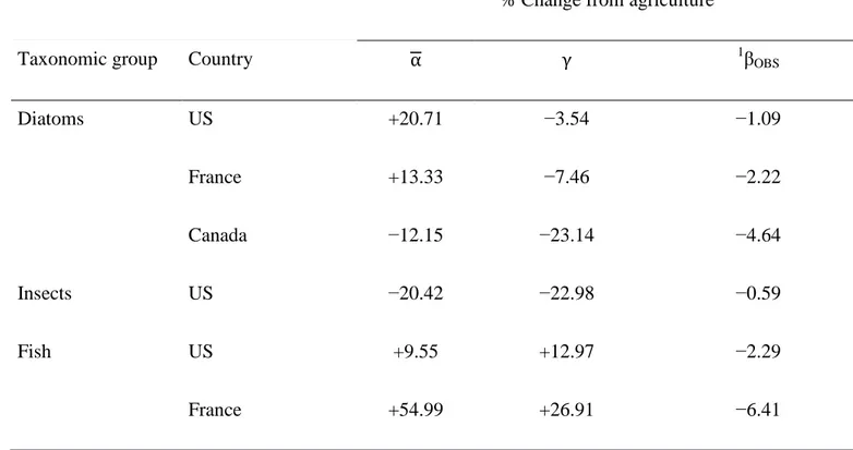
Table 2. Summary of the impact of agricultural land use on resampled diversity measures as positive or negative percent change relative to forest cover. Significant differences between land covers were detected in all comparisons (permutational MANOVA and ANOVA, P < 0.05).

% Change from agriculture

Taxonomic group Country α γ 1βOBS

Diatoms US +20.71 −3.54 −1.09 France +13.33 −7.46 −2.22 Canada −12.15 −23.14 −4.64 Insects US −20.42 −22.98 −0.59 Fish US +9.55 +12.97 −2.29 France +54.99 +26.91 −6.41 1_{β-diversity = 1 −} α γ

FIGURE LEGENDS

Figure 1. a. Conceptual model depicting the land use effect on the species abundance

distribution (SAD) and intraspecific spatial aggregation, which in turn interact with local (α) and regional (γ) diversity. β-diversity is calculated as a function of average α-diversity and

γ-diversity. Interactions that were controlled for by the null models of Kraft et al. (2011) and Xu et

al. (2015) are marked with a thick dotted line. b. Diagram summarizing the Xu et al. (2015)

partition of βDEV into fractions explained by the SAD and intraspecific spatial aggregation using an occupancy-abundance based null model procedure. The null model βDEV is taken as the raw difference between expected β-diversity (βEXP) and observed β-diversity (βOBS). The fraction of βDEV explained by the SAD, βSAD, is the difference between predicted β-diversity (βPRED) and expected β-diversity (βEXP), whereas the fraction of βDEV explained by intraspecific aggregation (βAGG) represents the difference between βOBS and βPRED.

Figure 2, a-f. Maps of diatom, macroinvertebrate, and fish sampling localities in the US, France, and Canada. Grey triangles represent agriculture samples, whereas black circles represent forest samples. a = US diatoms, b = US insects, c = US fish, d = French diatoms, e = French fish, f = Canadian diatoms.

Figure 3, a-f. Boxplots showing differences in resampled physicochemical heterogeneity between land covers for each dataset. a = US diatoms, b = French diatoms, c = Canadian diatoms, d = US insects, e = US fish, f = French fish. Points indicate resamples that fall outside

the interquartile range. Different letters denote significant differences in mean heterogeneity (permutational ANOVA, P < 0.05).

Figure 4, a-f. Boxplots of resampled SAD and null model metrics showing the differences between land covers for each dataset. a = US diatoms, b = French diatoms, c = Canadian diatoms, d = US insects, e = US fish, f = French fish. Significant differences were observed in all comparisons (permutational ANOVA, P < 0.05) except βDEV for US insects (panel D3, denoted by asterisk).

Figure 5, a-f. Venn diagrams showing output of redundancy analysis-based variance

partitioning of diversity measures (α-, β-, and γ-diversity). Values represent model adjusted R2 values. Values in intersections represent covariance fractions, whereas values in circles represent pure fractions.

Figure 6, a-f. Venn diagrams showing output of regression-based variance partitioning of βDEV. Values represent model adjusted R2 values. Values in intersections represent covariance

Figures

Figure 1

Figure 5

Figure 6

Supporting Information Appendix Short Titles

Appendix 1: Expanded description of environmental data and null model correlation results Appendix 2: Description of Null Model Machinery

Appendix 3: R-code script for looping procedures Appendix 4: R-code script for analyses of loop output