HAL Id: tel-02570431
https://pastel.archives-ouvertes.fr/tel-02570431
Submitted on 12 May 2020HAL is a multi-disciplinary open access archive for the deposit and dissemination of sci-entific research documents, whether they are
pub-L’archive ouverte pluridisciplinaire HAL, est destinée au dépôt et à la diffusion de documents scientifiques de niveau recherche, publiés ou non,
State � Glissement, Sismicité et Évolution de
Perméabilité
Michelle Almakari
To cite this version:
Michelle Almakari. Réactivation Hydro-Mécanique d’une Faille Rate & State � Glissement, Sismicité et Évolution de Perméabilité. Géologie appliquée. Université Paris sciences et lettres, 2019. Français. �NNT : 2019PSLEM065�. �tel-02570431�
Préparée à MINES ParisTech
Réactivation Hydro-Mécanique d’une Faille Rate & State:
Glissement, Sismicité et Évolution de Perméabilité.
Hydro-Mechanical Rate & State Fault Reactivation: Slip, Seismicity
and Permeability Enhancement.
Soutenue par
Michelle ALMAKARI
Le 18 Décembre 2019 École doctorale no398Géosciences
Ressources
Naturelle et Environnement
SpécialitéGéosciences et Géoingénierie
Composition du jury : Mr. Frédéric CAPPAProfesseur, Université Nice Sophia Antipolis Président Mr. Georg DRESEN
Professeur, University of Potsdam Rapporteur Mr. Hideo AOCHI
Cadre Scientifique des EPIC, BRGM Rapporteur Mr. Jean SULEM
Professeur, Ecole des Ponts ParisTech Examinateur Mme. Agnès Helmstetter
Chargée de Recherche, Univ. Grenoble Alpes Examinatrice Mr. Hervé CHAURIS
Professeur, MINES ParisTech Directeur de thèse Mr. Pierre DUBLANCHET
“In every end, there is also a beginning.”
A Great and Terrible Beauty
LIBBA BRAY
Acknowledgments
First, I would like to express my deepest appreciation and acknowledgments to my su-pervisors Pierre DUBLANCHET and Hervé CHAURIS for providing me the opportunity to conduct this thesis. Particularly, I thank Pierre for his guidance, support, constant supervision, as well as for all the long discussions that we had and his very clear explica-tions. I appreciate a lot the confidence that he had in my work and the freedom he gave me to chose the different directions that I want to explore during my thesis. I also thank him for giving me the opportunity to teach a few sessions of rock mechanics at IPGP, this experience was particularly interesting for me. I would also like to thank Hervé for being constantly involved in my thesis, even in the parts that are not within his area of expertise. I particularly enjoyed working with him to develop and apply the inversion approaches. Even though I had no previous extensive knowledge in this area, his clear explications and continuous guidance made everything look easy. So I thank him for that. Finally, beyond the scientific discussions, I would also like to thank Pierre and Hervé for their in-volvement, their advice in every discussion that we had concerning my professional project.
I would also like to thank François Passelègue (EPFL, Lausanne) with whom I had the chance to collaborate. This collaboration allowed me to explore the experimental world, which was new for me, and benefit from his large expertise in this area.
During this thesis, I benefited from a 3 years doctoral contract from MINES Par-isTech which allowed me to conduct my research in very good conditions, to which I am entirely grateful. I also had the chance to benefit from additional funding from the Paris Exploration Geophysics Group (GPX), which sponsored my participation to the 3rd international workshop on earthquakes in Cargèse in 2017 and to the EGU General
Assembley in Vienna in 2018. I also benefited from the French government program “Investissements d’Avenir” under the grant agreement n ANR-10-IEED-0801 (Project GIS Geodenergie/TEMPERER), which sponsored my participation to the AGU Fall Meeting in Washington, DC in 2018. Finally, I also thank the organisers of the Schatzalp 3rd
Induced Seismicity Workshop for giving me the opportunity to participate as a fellowship applicant in this workshop that took place in Davos, Switzerland in 2019.
My sincere thanks go to Harsha BHAT and Frédéric PELLET for taking part in my annual PhD committee. Their comments and recommendations allowed me to improve the quality of my work. I also thank Pierre-François ROUX and Alexandrine GESRET for the many fruitful discussions that we had.
DRESEN and Hideo AOCHI accepted to review my thesis in detail. I thank them in advance for their comments and recommendations. My sincere thanks also go to Jean SULEM, Frédéric CAPPA and Agnès HELMSTETTER for examining my work.
I am so grateful for the Geosciences center, and especially the geophysical team (Mark Noble, Alexandrine Gesret, Hervé Chauris, Pierre Dublanchet, Pierre-François Roux, Nidhal Belayouni and Véronique Lachasse). Thank you for welcoming me, and allowing me to conduct my thesis in very kind, friendly and warm conditions. I particularly thank Véronique Lachasse for always being there for me and for taking care of me when I twisted my ankle. I would also like to thank all my PhD colleagues for their friendship and support over the last three years: Yves Marie Batany, Emmanuel Cocher, Keurfon Lu, Yubing Li, Alexandre Kazantsev, Hao Jiang, Tianyou Zhou, Ahmed Jabrane, Milad Farshad (yes for a long time I was the only girl in the team!). And finally I thank deeply Rita Abou Jaoude for accompanying me during our long journey to-gether. I look forward to being there for you and with you at the day of your PhD defense.
I cannot forget the support of my family. I would not be here if it was not for my parents. Mom and Dad, thank you for your continuous encouragement, unconditional love and for always reminding me how proud you are of my achievements. Thank you for always having the curiosity to understand what I do. This means a lot to me. I also thank my brother and his wife for supporting me, and for constantly visiting me in France whenever they had the chance, the time that we spent together and the memories that we made mean a lot to me.
Last but not least my greatest gratitude goes to my fiancee. You are the reason why I am now at the finishing line of this PhD. Thank you for supporting me through-out my ups and downs. Thank you for believing in me, even when I had doubts in myself. Thank you for always having the time to listen and for being so understand-ing. I can never forget that you almost memorized my speech of “Ma Thèse en 180 secondes”, you were able to explain the context of my thesis in my place! Finally, thank you for always being there for me, many rough days have passed unnoticed because of you.
Abstract
This PhD thesis is dedicated to the study of injection induced fault reactivation using a coupled hydro-mechanical rate and state model of a fault. Even though the principal mechanisms behind induced fault reactivation are well known, different aspects are not yet fully explored, nor understood. In the first part of this thesis, we explore successively the role of the injection protocol (in particular, injection maximum pressure and injection pressure rate), and the fault frictional parameters on the rate of induced events and their magnitude content, for different heterogeneous 2-D fault configurations. We first point out a temporal correlation between the seismicity rate and the pore pressure rate governing the fault. We then show a dependence of the rate and magnitude content of the seismic events on the injection parameters, as well as the existence of an important trade-off between them, which could not be addressed using the Dietrich (1994)’s seismi-city rate model. Concerning the frictional parameters, we show that for the faults tested in this study, the ones having a more stable frictional behavior exhibit a lower induced seismicity rate and seismic moment released. In the last part of this study, the variation of the hydraulic diffusivity during fluid injection with shear slip and effective stress reduction is addressed. For this, we use laboratory injection experiments on an Andesite rock sample, during which the pore pressure was measured at two locations along the fault plane. In an inversion framework, we estimate the best model and the associated uncertainties of an effective diffusivity history that could explain the experimental data. Using this information, we could extend our hydro-mechanical model, which would allow the computation of pore pressure, diffusivity and slip changes along the experimental fault. Keywords: Fault Reactivation, Fluid Injection, Rate and State Fault Numerical Model, Induced Seismicity, Laboratory Rock Mechanics Experiments, Permeability Enhancement.
Resume
Cette thèse est dédiée à l’étude de la réactivation de faille par injection de fluide, à l’aide d’un modèle hydro-mécanique de faille rate and state. Bien que les principaux mécanismes à l’origine de la réactivation de faille soient bien connus, différents aspects ne sont pas encore complètement explorés, ni compris. Dans la première partie de cette thèse, on explore le rôle du protocole d’injection (en particulier, la pression maximale et le taux de pression d’injection), ainsi que le rôle des paramètres de frottement sur le taux de sismicité et la distribution de magnitude, pour différents types de failles 2-D hétérogènes. On souligne d’abord une corrélation temporelle entre le taux de sismicité et le taux de pression de pore gouvernant la faille. On montre ensuite une dépendence du taux de sismicité ainsi que de la distribution des magnitudes sur les paramètres d’injection. Notamment, une compensation entre ces deux existe pour de grandes valeurs du taux de pression d’injection. Ce comportement ne peut pas être abordé par le taux de sismicité proposé par Dietrich (1994). En outre, on montre que les failles ayant un comportement de frottement plus stable présente un taux de sismicité et un moment sismique libéré plus faibles. Dans la dernière partie de cette étude, la variation de la diffusivité hydraulique au cours de l’injection de fluide avec l’accumulation du déplacement et la réduction de la contrainte normale effective sur la faille est abordée. Pour cela, on utilise des expériences d’injection (réalisées à l’échelle du laboratoire) sur un échantillon d’andésite, où la pression de pore est mesurée à deux endroits le long de la faille. En appliquant des méthodes d’inversion, on estime le meilleur modèle de diffusivité hydraulique et les incertitudes associés, pouvant expliquer les données expérimentales. Avec ces résultats, on peut étendre notre modèle hydro-mécanique, afin de pouvoir calculer la pression de pore, la diffusivité hydraulique et le déplacement accumulé sur la faille expérimentale.
Mots Clés: Réactivation de Faille, Injection de Fluide, Modèle Numérique de Faille Rate and State, Sismicité induite, Expériences de Laboratoire, Évolution de Pérméabilité.
Contents
Acknowledgments iii
Abstract v
Resume vii
Chapter 1 Introduction – Fault reactivation due to fluid injection 1
1.1 General Introduction . . . 3
1.2 Industrial Injection Projects and Fault Activation . . . 4
1.2.1 Waste Fluids Disposal (WD) . . . 4
1.2.2 Production of Geothermal Energy (EGS) . . . 4
1.2.3 Hydrofracturing (HF) . . . 5
1.2.4 CO2 Injection . . . 5
1.2.5 Secondary recovery of oil and gas or enhanced oil recovery (EOR) 5 1.3 Discrimination between Induced and Natural Seismicity . . . 5
1.4 Observations of Injection Induced Fault Reactivation . . . 7
1.4.1 Observations of Induced Earthquakes . . . 7
1.4.2 Temporal Correlation and Post Shut-in Seismicity . . . 15
1.4.3 Spatial Migration of events . . . 18
1.4.4 Magnitude Content . . . 19
1.4.5 Effect of Injection Parameters . . . 21
1.4.6 Evidence of Induced Aseismic Motion . . . 22
1.5 Managing Induced Seismicity . . . 24
1.6 First Conceptual Models For Fluid Induced Fault Reactivation . . . 27
1.7 Injection Experiments for Better Understanding Fault Reactivation and Induced Seismicity . . . 30
1.7.1 Large Scale In-situ Injection Experiments . . . 30
1.7.2 Decametric Scale Injection Experiments: Seismicity and Aseismic Slip . . . 31
1.7.3 Small Scale Laboratory Injection Experiments . . . 32
1.8 Contributions from different Numerical Modeling Approaches . . . 36
1.8.1 Pressure diffusion based models . . . 36
1.8.2 Injection into rock volumes with Coulomb failure criterion . . . 38
1.8.3 Numerical models based on Fracture Mechanics . . . 38
1.8.4 Models following the seismicity rate model proposed by Dietrich (1994) . . . 39
1.8.6 Frictional Fault Models . . . 40
1.9 Research Motivation . . . 42
1.10 Thesis and Manuscript Overview . . . 44
Chapter 2 Effect of the injection scenario on the rate and magnitude content of injection-induced seismicity: Case of a heterogeneous fault 49 2.1 Abstract . . . 51
2.2 Introduction . . . 51
2.3 Model . . . 53
2.4 Results . . . 61
2.4.1 Background Seismicity . . . 61
2.4.2 Response to Fluid Injection . . . 61
2.4.3 Sensitivity Analysis . . . 64
2.4.3.1 Choice of Injection Parameters . . . 64
2.4.3.2 Time of Maximum Seismicity Rate and Seismicity Per-turbation Duration . . . 65
2.4.3.3 Seismicity Rate Increase . . . 66
2.4.3.4 Magnitude Content . . . 69
2.4.3.5 Seismic Moment Release and number of earthquakes dur-ing Phase I, Phase II, and Phase (I–II) . . . 71
2.4.3.6 Change in Diffusive Boundary Conditions . . . 73
2.5 Discussion . . . 75
2.6 Conclusion . . . 79
2.7 Appendix A: Analytical Solution of the Diffusion Equation . . . 80
2.7.1 Injection Phase 1 (ti < t < tr): . . . 80
2.7.2 Injection Phase 2 (tr < t ): . . . 80
2.8 Appendix B: Estimation of the Background Stressing Rate . . . 80
2.9 Appendix C: Analytical Seismicity Rate model following Dietrich (1994) . 81 2.9.1 Injection Phase 1 (ti < t < tr): . . . 82
2.9.2 Injection Phase 2 (tr < t): . . . 82
2.10 Supporting Information . . . 82
Chapter 3 Sensitivity of Induced Seismic Activity to Fault Frictional Parameters 89 3.1 Introduction . . . 91
3.2 Fault Configurations . . . 93
3.3 Results . . . 94
3.3.1 Quick Overview of the Background Seismicity . . . 94
3.3.2 Seismic Response to Fluid Injection . . . 96
3.3.2.1 Phase I . . . 96
3.3.2.2 Phase II . . . 100
3.4 Discussion . . . 101
3.5 Conclusion . . . 103
Contents
Chapter 4 Deterministic and Probabilistic Inversions of Pore Pressure Diffu-sion: Application to Laboratory Injection Experiments 107
4.1 Introduction . . . 109 4.2 Experimental Data . . . 111 4.2.1 Experimental Setup . . . 111 4.2.2 Experimental Protocol . . . 113 4.2.3 Experimental Results . . . 113 4.3 Methodology . . . 115 4.3.1 Inverse Problem . . . 115 4.3.2 Deterministic inversion . . . 118
4.3.2.1 Adjoint State Method (Gradient method): Theory . . . . 118
4.3.2.2 Resolution of the Differential Equations . . . 119
4.3.2.3 Numerical Implementation . . . 120
4.3.3 Metropolis Hastings Algorithm . . . 122
4.3.3.1 Theory and Resolution . . . 122
4.3.3.2 Numerical Implementation . . . 123
4.4 Application to the Experimental Data . . . 125
4.4.1 Estimating the Best Model: Deterministic Approach . . . 125
4.4.2 Estimating the Uncertainties: the MCMC approach . . . 130
4.4.3 Discussion . . . 134
4.5 Diffusivity, Displacement and Effective Stress . . . 135
4.6 Conclusion and Perspectives . . . 140
4.7 Appendix A: Development of the Adjoint State Method . . . 141
Chapter 5 Conclusions and Perspectives 145 5.1 General Conclusion . . . 147
5.2 Perspectives . . . 148
5.2.1 Post Shut-in Seismicity . . . 148
5.2.2 Modeling Induced Aseismic Motion and Second Order Triggering of Seismic Failure . . . 149
5.2.3 Hydro-Mechanical Modeling of Laboratory Injection Tests . . . 149
List of Figures
1.1 Discrimination of natural and induced seismicity, method byDavis and
Frohlich (1993) . . . 6
1.2 Induced earthquakes between 2006 and 2017 (Keranen and Weingarten, 2018). . . 8
1.3 Number of earthquakes per year in the central U.S (Source: USGS). . . . 10
1.4 Temporal correlation (Dorbath et al., 2009;Kozlowska et al., 2018) . . . . 17
1.5 Migration of induced events away from the well (Shapiro et al., 1997) . . 19
1.6 Change in magnitude content (Skoumal et al., 2014; Schoenball et al., 2015;Goebel et al., 2016a;Goebel et al., 2016b) . . . 20
1.7 Maximum magnitude and injected volume (McGarr, 2014;Van der Elst et al., 2016) . . . 21
1.8 Effect of injection parameters on features of induced seismicity (Raleigh et al., 1976;Langenbruch et al., 2018) . . . 23
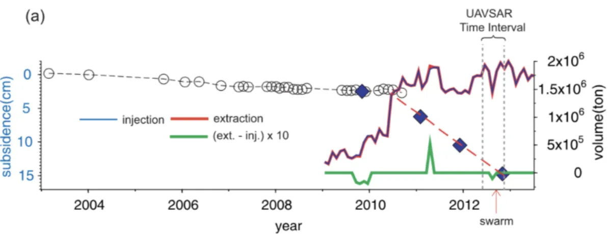
1.9 Evidence of aseismic deformation during the Brawly swarm in 2012 (Wei et al., 2015) . . . 24
1.10 Traffic light systems and earthquake magnitudes (Deichman and Giardini, 2009;Kwiatek et al., 2019) . . . 26
1.11 Mechanisms for inducing earthquakes (Ellsworth, 2013) . . . 27
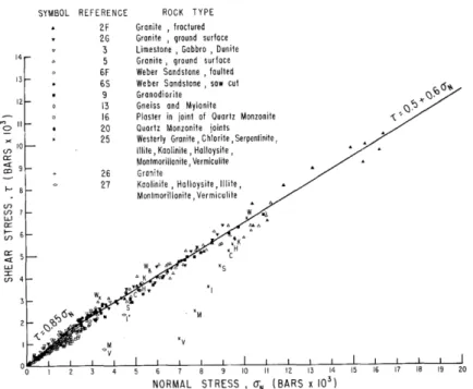
1.12 Shear stress as a function of normal stress for a variety of rock types Byerlee (1978) . . . 28
1.13 Conceptual model of induced fault reactivation. . . 29
1.14 Evidence of aseismic slip from in-situ injection experiments (Guglielmi et al., 2015b) . . . 32
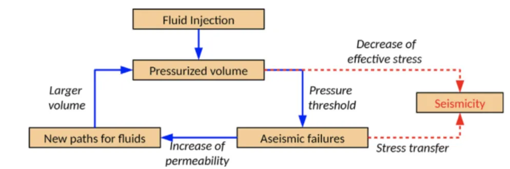
1.15 Proposed model for injection induced seismicity (De Barros et al., 2018) . 33 1.16 Injection energy plotted against seismic energy (Goodfellow et al., 2015) . 34 1.17 Sketch of fluid injection and fluid flow into a rock medium containing pre-existing fractures. . . 37
2.1 Fault Model . . . 55
2.2 Pore pressure diffusion . . . 58
2.3 Seismic activity: before and during fluid injection . . . 63
2.4 Time of maximum seismicity rate and seismicity perturbation duration. . 66
2.5 Dependence of the seismicity rate increase on the injection parameters . . 68
2.6 Dependence of the moment magnitude distribution on the injection para-meters . . . 70
2.7 Evolution of the b-value with the injection parameters . . . 72
2.9 Estimation of the background stressing rate . . . 81
2.10 Time series of the moment magnitudeMw for different injection scenarios. 83 2.11 Time series of the cumulative number of earthquakes and the seismic moment for different injection scenarios. . . 84
2.12 Seismicity rate and injection history for different injection scenario, part 1. 85 2.13 Seismicity rate and injection history for different injection scenario, part 2. 86 2.14 Comparison between different boundary conditions.. . . 87
3.1 Fault configurations: Along strike distribution of the critical slip distance dc and the ratio of frictional parameters a/b. . . . 95
3.2 Dependence of the seismicity rate increase on the injection parameters for different fault configurations. . . 98
3.3 Variation of the average seismic moment rate with the injection parameters for different fault configurations. . . 99
3.4 Number of earthquakes and moment magnitude released during Phase II of injection, for the different fault configurations. . . 101
3.5 Background seismicity for the different fault configurations. . . 104
3.6 Dependence of the magnitude distribution on the injection parameters, for the different fault configurations. . . 105
3.7 Spatial distribution of the seismic rupture for fault configuration 5. . . 106
4.1 Experimental Setup. . . 112
4.2 Experimental results: pressure and average displacement . . . 114
4.3 Experimental results: Deformation . . . 116
4.4 Flow Chart: Deterministic approach . . . 121
4.5 Flow Chart: Metropolis Hastings Method . . . 124
4.6 Results of the Deterministic Approach for the experiment at Pc = 30 MPa.127 4.8 Results of the Deterministic Approach for the experiment at Pc = 95 MPa.128 4.9 Results of the Deterministic Approach for the experiment at Pc = 60 MPa.129 4.11 Results of the MCMC Method for the experiment at Pc = 30 MPa. . . 131
4.12 Results of the MCMC Method for the experiment at Pc = 60 MPa. . . 132
4.13 Results of the MCMC Method for the experiment at Pc = 95 MPa. . . 133
4.14 Diffusivity and Effective Stress . . . 136
4.15 Relationship between the square of the ratio of the hydraulic diffusivity to the initial diffusivity and the logarithm of the ratio of the mean ef-fective stress to the initial efef-fective stress: at 30 MPa in the range [300 – 700] seconds, 60 MPa in the range [700 – 1400] seconds and 95 MPa in the range [2000 – 4200] seconds. Different colors refer to the different confining pressure values. Diffusivity values are issued from the deterministic method.138 4.16 Diffusivity and Displacement . . . 139
4.17 Validation of the Gradient Estimation . . . 144
5.1 Numerical hydro-mechanical modeling of the laboratory injection test at 30 MPa of confining pressure. . . 150
List of Tables
1.1 List of potentially induced earthquakes. . . 16
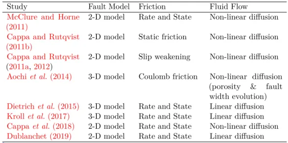
1.2 List of the main components of some frictional fault models.. . . 41
2.1 Numerical Simulations: List of physical parameters . . . 60
3.1 Characteristics of the different fault configurations. . . 94
3.2 Background seismicity for the different fault configurations. . . 96
4.1 Laboratory Injection Experiment: List of geometrical and mechanical parameters.111 4.2 Laboratory Injection Experiment: List of experimental parameters. . . 113
Chapter 1
Introduction – Fault reactivation due to
fluid injection
Contents
1.1 General Introduction . . . 3
1.2 Industrial Injection Projects and Fault Activation . . . 4
1.2.1 Waste Fluids Disposal (WD) . . . 4
1.2.2 Production of Geothermal Energy (EGS) . . . 4
1.2.3 Hydrofracturing (HF) . . . 5
1.2.4 CO2 Injection . . . 5
1.2.5 Secondary recovery of oil and gas or enhanced oil recovery (EOR) 5 1.3 Discrimination between Induced and Natural Seismicity . . . 5
1.4 Observations of Injection Induced Fault Reactivation. . . 7
1.4.1 Observations of Induced Earthquakes . . . 7
1.4.2 Temporal Correlation and Post Shut-in Seismicity. . . 15
1.4.3 Spatial Migration of events . . . 18
1.4.4 Magnitude Content . . . 19
1.4.5 Effect of Injection Parameters . . . 21
1.4.6 Evidence of Induced Aseismic Motion . . . 22
1.5 Managing Induced Seismicity . . . 24
1.6 First Conceptual Models For Fluid Induced Fault Reactivation. . . . 27
1.7 Injection Experiments for Better Understanding Fault Reactivation and Induced Seismicity . . . 30
1.7.1 Large Scale In-situ Injection Experiments . . . 30
1.7.2 Decametric Scale Injection Experiments: Seismicity and Aseis-mic Slip . . . 31
1.7.3 Small Scale Laboratory Injection Experiments. . . 32
1.8 Contributions from different Numerical Modeling Approaches . . . . 36
1.8.1 Pressure diffusion based models . . . 36
1.8.2 Injection into rock volumes with Coulomb failure criterion . . 38
1.8.4 Models following the seismicity rate model proposed byDietrich (1994) . . . 39
1.8.5 Burridge-Knopoff based models (Burridge and Knopoff, 1967) 40
1.8.6 Frictional Fault Models . . . 40
1.9 Research Motivation . . . 42
1.10 Thesis and Manuscript Overview . . . 44
Résumé du Chapitre 1 en Français
Certaines activités industrielles peuvent activer des failles pré-existantes et induire du glissement lent (asismique) ou du glissement rapide (sismique) dans le cas des séismes. Parmis ces activités industrielles, on peut citer: les activités minières, le remplissage des grands lacs de barrage ou l’injection de fluide dans le sous-sol associé à des projets d’énergie, comme par example la géothermie. Cependant l’injection de fluide présente le plus grand risque sismique, comme elle était la cause de plusieurs grands séismes induits, à titre d’éxample: le séisme de magnitude 5.5 à Denver Colorado en 1967, le séisme de magnitude 5.7 à Prague Oklahoma en 2011 et le séisme de magnitude 5.5 à Pohang City en Corée du Sud. Pour cette raison, on s’intéresse dans cette thèse à l’étude de la réactivation des failles par injection de fluides.
Dans ce chapitre d’introduction, je présente l’état de l’art sur (1) les différentes activités industrielles d’injection de fluide dans le sous-sol qui engendrent une sismicité induite, (2) les méthodes actuelles de discrimination entre sismicité naturelle et induite, (3) les observations de cas réels ainsi que les différentes caractéristiques de la sismicité induite, (4) les méthodes actuelles et les efforts visant à minimiser le risque de la sismicité in-duite. Ensuite je présente (5) les premiers modèles de la réactivation induite des failles, (6) les différentes études expérimentales d’injection de fluide (à différentes échelles) et les différentes réponses qu’elles ont pu apporter, ainsi que (7) les différents modèles numériques proposés et leur contributions majeures. Finalement, j’expose (8) mes mo-tivations pour ce travail de recherche, ainsi que (9) l’organisation de la thèse et mes contributions majeures.
1.1 General Introduction
1.1 General Introduction
We say that a fault is reactivated when slip nucleates along it. If the slip is fast, often called dynamic slip, it can generate seismic waves that can reach the earth’s surface. This is what we call a seismic event or earthquake. On the other hand, if the slip is slow, it does not generate any seismic waves, and is called slow slip or aseismic slip.
A seismic event is characterized by the surface of the rupture S and the rupture dis-placement δ. These parameters allow to estimate the seismic moment of the earthquake M0 = µ S δ, where µ represents the rigidity of the rocks (Aki, 1966). The seismic
moment is a measure of the energy released by the earthquake. Kanamori (1977) then introduced the earthquake magnitude Mw as a dimensionless characteristic to describe
the size of the earthquake as follows: Mw = 2/3 log10(M0) - 6.07, where M0 is expressed
in Newton meters.
Beyond natural conditions, it has been acknowledged that some human anthropogenic activities can lead to subsurface stress changes, reactivating pre-existing faults and indu-cing aseismic motion and minor as well as large earthquakes (Ellsworth, 2013;Keranen and Weingarten, 2018).
Induced seismic activity can be caused by mining activities (McGarr et al., 2002;
Gibowicz, 2009) like the Belchatow, Poland earthquake in 1980 (Gibowicz, 1984) and the magnitude 5.5 earthquake that stroke Orkney in South Africa in 2014 (Bateman, 2014). Impoundment of deep reservoir lakes in tectonically active regions can also in-voke earthquakes that can be damaging (Simpson and Leith, 1988). For instance the deadly 1967 magnitude 6.3 earthquake in Koyna, India was directly related to Koyna dam reservoir (Gupta, 2002). The 1962 magnitude 6.1 earthquake in Hsingfenkiang, China, the 1963 magnitude 5.8 earthquake in Karib, Zimbabwe and the 1966 magnitude 6.3 earthquake in Kremasta, Greece were also linked to lake level changes (Simpson, 1976). However, nearly the majority of induced earthquakes are linked to energy projects associated with fluid injection. This has become a focus of present research studies and discussions (Ellsworth, 2013), and it is likely to continue as further developments carry on in the industrial, energy related, activities (Keranen and Weingarten, 2018). Injection activities were responsible of some large induced seismic events, like the 1967 Mw 5.5 in Denver Colorado (Healy et al., 1968; Davis and Frohlich, 1993), the 2011 Mw 5.7 earthquake in Prague Oklahoma (Keranen et al., 2013;Van der Elst et al., 2013; McGarr, 2014;Sumy et al., 2014) and the 2017Mw 5.5 earthquake in Pohang city, South Korea (Kim et al., 2018;Grigoli et al., 2018).
Nonetheless, induced seismic events are not the only seismic outcome from fluid in-jection, it may sometimes induce some aseismic slip, which was observed during in-situ injection experiments (Guglielmi et al., 2015b;Duboeuf et al., 2017) as well as during real injection activities (Bourouis and Bernard, 2007; Wei et al., 2015; Cornet, 2016). In
this case, induced aseismic slip is suspected to trigger earthquakes as an indirect effect of fluid injection (De Barros et al., 2018).
As injection activities appear to pose the higher risk on seismic hazard, we focus in this thesis on fault reactivation due to fluid injection. The induced fault reactivation is not yet controlled nor fully understood. The aim of this chapter is to present a broad, but not exhaustive, (1) review of different industrial injection activities inducing seismicity, (2) current methods to discriminate between natural and induced seismicity, (3) observations made from real cases, (4) efforts to manage induced seismicity and minimize its risk, (5) the first conceptual models for fluid induced fault reactivation, (6) advances from injection experiments at different scales, and (7) contributions from previous numerical modeling studies. We then (8) expose our motivations for this work, (9) present the thesis organization, and finally (10) point out our major contributions.
1.2 Industrial Injection Projects and Fault Activation
Several industrial injection projects give rise to micro-seismicity as well as to some large seismic events. They do not pose the same risk to seismic hazard though.
1.2.1 Waste Fluids Disposal (WD)
Disposal of waste fluids is widely used in the United States (Ellsworth, 2013), often related to hydraulic fracturing projects. It is suspected to be responsible for the large increase in the seismicity rate in the Central U.S. (Oklahoma, Arkansas, Colorado, Kansas) (Keranen et al., 2014;Rubinstein and Mahani, 2015;Goebel et al., 2016a), as well as for some of the largest induced earthquakes (Keranen et al., 2014; Rubinstein and Mahani, 2015; Yeck et al., 2016). Some authors suggest that among the different injection activities waste fluid disposal poses the highest risk to seismic hazard as it operates for longer times (Ellsworth, 2013), and it injects a large volume of fluids (Horton, 2012;
Keranen et al., 2013;Frohlich et al., 2014;Rubinstein et al., 2014).
1.2.2 Production of Geothermal Energy (EGS)
Production of geothermal energy takes part of the sustainable energy plan and is vastly used worldwide. However, geothermal systems were responsible for induced seismic swarms in Krafla (Tang et al., 2008; Evans et al., 2012) and Hengill (Bjornsson, 2004;
Axelsonn, 2006) in Iceland, in Soutz-sous-Forêt, France with magnitudes up to 2.9 (Majer
et al., 2007;Dorbath et al., 2009) and in the Rittershoffen deep geothermal reservoir in
Northeast of France (Lengline et al., 2017), as well as large earthquakes, for instance the 1982 magnitude 4.6 earthquake in Geysers, United States (Majer et al., 2007) or the four magnitude 3 earthquakes in 2006 at 3 km depth under the city of Basel in Switzerland (Deichman and Giardini, 2009) that lead to the abandonment of the project, the magnitude 3.5 earthquake in 2013 in St. Gallen, Switzerland (Diehl et al., 2017),
1.3 Discrimination between Induced and Natural Seismicity
and recently the magnitude 5.4 earthquake in 2017 near Pohang City (Kim et al., 2018;
Grigoli et al., 2018).
1.2.3 Hydrofracturing (HF)
Hydraulic fracturing of rocks is used to enhance the permeability of reservoirs (Holland, 2011; Kanamori and Hauksson, 1992). Among many others, it induced a series of earthquakes with a maximum magnitude of 2.3 near Blackpool, United Kingdom (Green
et al., 2012), the magnitude 3.8 earthquake in the Horn River Basin of British Columbia
that was felt by local population (Farahbod et al., 2015) and the magnitude 4.2 earthquake in Fox Creek Alberta in Western Canada (Atkinson et al., 2016). Shapiro et al. (2010)
argues that it poses lower probability of inducing large events than in waste fluid disposal and production of geothermal energy as hydraulic fracturing activities operate for a short duration and do not inject large volume of fluids.
1.2.4 CO2 Injection
CO2 is injected into deep formations for permanent carbon capture and storage (CCS).
Even though it poses non negligible seismic hazard, there exists to few projects (Zobak and Gorelick, 2012). According to Rutqvist et al. (2016), no felt seismic event was recorded to date resulting from CO2 storage projects, even though CO2 injection in the
Cogdell field was suspected to have induced the 2011 magnitude 4.4 earthquake near Snyder, Texas (Gan and Frohlich, 2013).
1.2.5 Secondary recovery of oil and gas or enhanced oil recovery (EOR)
Secondary recovery of oil and gas can also invoke earthquakes (Davis and Pennington, 1989), mainly low magnitude earthquakes too small to be felt (McGarr et al., 2015). It was responsible of a series of small (magnitude lower than 3.5) and shallow earthquakes due to the extraction of natural gas in the Netherlands from shallow deposits (Van Eck
et al., 2006).
1.3 Discrimination between Induced and Natural Seismicity
The identification of an induced event may be a complicated job, especially in tecton-ically active regions (Goebel et al., 2016b), in which many naturally seismic sequences occur. This is particularly the case, if standards seismicity catalogs with high magnitude of completeness are used. Davis and Frohlich (1993)proposed a list of criteria to evaluate the nature of an event, or to assess the seismic hazard of a future project. In the case of a past event, these criteria depend on the background seismicity, the injection practices and the temporal and spatial correlation between the injection activity and the recorded seismicity. The method is presented in Figure 1.1and consists of a list of “yes” or “no” questions, to which the user answers. A simple count in the end of all the different answers gives an insight on the nature of the seismic event in question. However, in thismethod each question is treated equally, regarding its actual importance, without any information about the uncertainties or the evidence. This is why Verdon et al. (2019)
extended this method by replacing the “yes” or “no” questions with positive and negative scores, that are modulated with respect to the importance of the question and to the degree of uncertainty. This method allows to estimate an induced assessment ratio that indicates whether the event is induced or not, and an evidence strength ratio that gives an idea about the uncertainty of the result.
Figure 1.1 – Discrimination of natural and induced seismicity: Series of seven “yes" or “no" questions to assess whether a certain earthquake was induced by fluid injection
activities, from (Davis and Frohlich, 1993).
Systematic differences in the seismicity rate between natural and induced seismic activities in Oklahoma and Arkansas were reported, typically an increase in background seismicity and a change in the fraction of main shocks (Llenos and Michael, 2013). In the same spirit, Goebel et al. (2016a)proposed a statistical approach based on the concept
1.4 Observations of Injection Induced Fault Reactivation
of clustering in time and magnitude, relying on the background seismicity rate and the magnitude content of the seismic events. The latter is generally characterized by the slope, called b-value, of the magnitude frequency distribution: log(N(m >M)) = a − bM,
whereN is the number of earthquakes per unit of time having a magnitude m >M, a
is a background seismicity indicator and b represents the ratio between large and small earthquakes and is typically around 1 for natural seismicity (Gutenberg and Richter, 1954). Goebel et al. (2016a)argued that an increase in the background seismicity rate and a decrease of the b-value could indicate the fault reactivation through induced seismicity. However, no difference in the magnitude distribution and inter-event times between natural and induced seismicity was observed for the Coso geothermal field in California (Schoenball et al., 2015).
1.4 Observations of Injection Induced Fault Reactivation
1.4.1 Observations of Induced Earthquakes
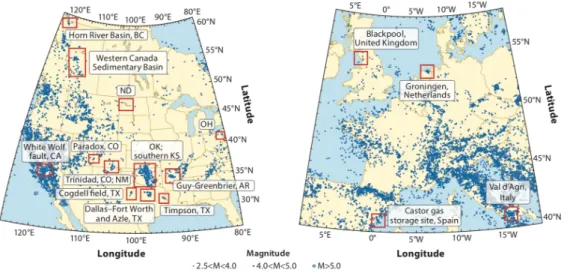
As mentioned before injection induced seismicity has become an important subject of research and discussion worldwide, as industrial injection activities are inducing micro-seismicity as well as large seismic events all over the globe. In an annual review about induced seismicity,Keranen and Weingarten (2018) presented a map with the location of injection induced earthquakes between 2006 and 2017 in the United States, Canada and Europe (Figure1.2), pointing out the severity of the situation. In this section, we attempt to briefly review some of the major induced (or potentially induced) seismic events by fluid injection activities, and expose the main reasons of why they were suspected to be induced.
Denver Colorado, United States
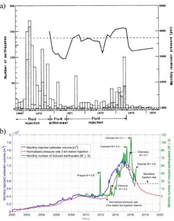
One of the first well documented cases of injection induced seismicity was in Rocky Mountain Arsenal in Denver Colorado, where waste contaminated water was injected into a deep well under pressure from 1962 to 1966, with a one year shut in period between 1963 and 1964 (Evans, 1966; Healy et al., 1968). 710 earthquakes with magnitudes in the range [0.7 – 4.3] were recorded during the injection period between 1962 and 1965 within an 8 km radius from the well (Evans, 1966). This seismic sequence was suspected to be injection-induced due to the lack of evidence of similar seismic activity in the area before the waste injection started in 1962 (Healy et al., 1968). Moreover, Evans (1966)found a correlation between the average monthly injection volume and earthquake frequency. Seismic activity did not stop however after injection shut-in in February 1966, earthquakes continued at an average of 4 to 71 earthquakes per month, suggesting a link between the bottom well fluid pressure and the level of seismic activity (Healy
et al., 1968). The three largest earthquakes induced were recorded in 1967, 18 months
after injection ceased, with a maximum magnitude of 5.5 (Hermann et al., 1981). In an attempt to better understand the relation between the pore pressure and the frequency of induced earthquakes, an in-situ injection experiment was conducted at the Rangely oil field in Denver Colorado in 1969. This will be discussed in section 1.7.1.
Figure 1.2 – Locations of some induced earthquakes since 2006 and up to 2017 for the United States and Canada (left panel) and Europe (right panel), (Keranen and Weingarten, 2018)
Texas, United States
Injection of fluids for secondary recovery of oil in the Cogdell oil field in West of Texas (between 1957 and 1982) led to a sequence of induced earthquakes that started in 1974 and lasted for about 8 years (Davis and Pennington, 1989). Even though a long time delay, of around 17 years, was observed between the start of injection and the onset of seismic activity, the earthquakes occurred within an array of injection wells, and thus they were suspected to be induced by the injection activities. Davis and Pennington (1989)argued that time is needed for fluid pressure to build up and reach a critical value on a pre-existing fault which could explain the observed time lag. No significant seismic activity was detected in the area after injection stopped in 1982. However, starting in 2004 CO2was injected into the Cogdell field, and was suspected to have induced a seismic
sequence of 93 earthquakes between 2009 and 2011, with the largest being the 2011 Mw 4.4 earthquake near Snyder. The earthquake epicenters were spread within a 2 km radius area from actively injection wells, and correlated in time with significant increases inCO2
injection (Gan and Frohlich, 2013).
Hydraulic fracturing operations near the Dallas-Fort Worth Airport in Texas, an area with no previous historical earthquakes, induced a sequence of 10 small earthquakes in 2008 that were felt by the local population. The recorded earthquakes were less than 500 meters away and 200 meters deeper than the injection well (Frohlich et al., 2011). On the other hand, earthquake activity began only 6 weeks after hydraulic fracturing started in Barnet Shale Texas in 2009, within 3.3 km of one or more of the high rate injection wells, while no seismicity was recorded next to other high rate injection wells
1.4 Observations of Injection Induced Fault Reactivation
(Frohlich, 2012). Analyzing the seismic activity induced in this area between 2009 and 2011,Frohlich (2012)found that increasing injection rate beyond a critical site dependent rate can induce earthquakes if the fluid can reach a suitably oriented fault. Moreover, seismic activity continued in Barnet Shale long after injection stopped in 2009. According to Shapiro and Dinske (2009) post injection seismicity in this case corresponds to a non-linear pressure diffusion throughout the medium surrounding the fault, accompanied by permeability enhancement.
Oklahoma, United States
Oklahoma and the Central U.S. have become one of the major evidence of injection in-duced seismicity and it caught the attention of several researchers and motivated different observational, theoretical and numerical studies (e.g. Keranen et al. (2013), Ellsworth
(2013),Keranen et al.(2014),Goebel et al.(2016a),Langenbruch and Zoback(2016),Yeck
et al.(2016),Schoenball and Ellsworth(2017),Schoenball et al.(2018),Langenbruch et al.
(2018),Norbeck and Rubinstein(2018) andJohann et al.(2018)). Disposal of waste fluids via injection started in 1993 at zero well head pressure and then the latter was increased in steps of around 0.2 MPa in 2001 reaching 3.6 MPa in 2006 (Keranen et al., 2013). Figure 1.3represents the diagram of the number of earthquakes per year with magnitude three or larger. It shows that the Central U.S. had a low background seismicity rate with an average of 20 – 25 magnitude three or larger earthquakes per year, but then seismic activity experienced a very large increase in 2009 and peaked in 2015, with a total of 3427 (M≥3) earthquakes between 2009 and 2018. Seismic activity within Oklahoma experi-enced a 40 fold increase as compared to seismicity between 1976 and 2007 (Keranen et al., 2014). According to McGarr et al. (2015), the frequency of earthquakes in Oklahoma with magnitudes greater than 3 (Mw ≥3) exceeded the one in Californa in 2014, one of the most active seismic regions in the United States (Alden, 2018). This abrupt change in seismicity rate is one of the main arguments to prove that the increase in seismicity in this area is mainly related to waste disposal activities. Seismic activity in Central U.S. started near injection wells and then experienced a broad spatial spread, with events migrating northeast, away from the injection wells, at 0.1 km per day (Keranen et al., 2014). More than 200 earthquakes were recorded 20 km East of Oklahoma City between 2009 and 2011. Beyond the large increase in seismicity rate, several large earthquakes are potentially induced by the fluid injection activities in Oklahoma, like the Mw 5.7 earthquake se-quence in November 2011 near Prague, 5 years after the largest increase in well head pressure, and that was felt in 17 states (Keranen et al., 2013), and more recently the 2016 Mw 5.1 near Fairview, located 12 km from high rate injection wells and that was a part of a two years seismic sequence composed by 63 foreshocks and 89 aftershocks, with moderate magnitudes (Yeck et al., 2016;McGarr and Barbour, 2017) and the 2016
Mw 5.8 earthquake in Pawnee, felt across 7 midwestern states, and that was part of a seismic sequence of small earthquakes (Yeck et al., 2016).
Moreover, a short hydraulic fracturing operation took place in January 2011 in South Central Oklahoma and lasted 7 days. A sequence of 116 earthquakes was detected in the
area. It started 24 hours after the hydraulic fracturing operation began, with magnitudes ranging between 0.6 and 2.9, and presented a strong temporal and spatial correlation with the injection and thusHolland (2013)argues that this sequence is not related to the waste disposal activity but induced by the fracking activity.
Figure 1.3 – Diagram of the number of earthquakes per year in the cent-ral U.S. The area which experienced the largest increase in activity since 2009 is the red cluster at the center of the map. (Source: USGS - ht-tps://earthquake.usgs.gov/research/induced/overview.php)
Southern Kansas, United States
Disposal of waste fluids in Southern Kansas led the seismic activity to rise dramatically in 2013 with around 1000 earthquakes having magnitudes larger than 2 and 6 with magnitudes exceeding 4, recorded between 2013 and 2016 (Rubinstein et al., 2018). The 4.9 Milan earthquake was the largest in the sequence (Choy et al., 2016). Those events were considered as injection induced since no earthquakes of magnitude 4 were ever recorded in the area from 1974 to 2012; moreover the seismic activity exhibited temporal correlation with the injected volume and a spatial correlation with the injection wells (Rubinstein et al., 2018). Shortly after injection stopped, seismicity subsided near the
high rate injection wells, however it remained long after away from the well. Arkansas, United States
A swarm of hundreds of earthquakes began only a few months after disposal of hydrofracturing waste fluids started in 2009 in Arkansas. The reactivation of the Guy-Greenbrier fault led to 3 large earthquakes (Mw 4, 3.8, 3.9) in 2010 that were widely felt
1.4 Observations of Injection Induced Fault Reactivation
across the state. A second swarm initiated in February 2011 with the largest earthquake in the sequence being the Mw 4.7 earthquake. The seismicity rate showed a strong correlation with the injected volume (Horton, 2012). This rose the public concern and led to the shut down of the project. Even though earthquakes continued after shut down, the seismicity rate and the magnitude of the events dropped within three months. Ohio, United States
Wastewater from hydraulic fracturing in the Northeastern U.S were transported and injected near Youngstown Ohio, a region with no known earthquakes in the past, under high pressure up to 17 MPa. This led to a seismic sequence that initiated 13 days after injection started and were composed of 167 induced earthquake during injection in 2011 with magnitudes up to 3.9, that initiated close to the well and then migrated away (Kim, 2013). Frequency of earthquakes was mainly correlated with the daily injection volume and injection pressure and several short period of quiescence were observed following shut-in durshut-ing the holidays and weekends. Post shut-injection seismicity contshut-inued but decreased in rate and magnitudes within month after shut in. TheMw 3.9 earthquake, largest in the sequence, was recorded 24 hours after shut in though (Kim, 2013;Skoumal et al., 2014). Different sequences of induced seismic activity stroke the eastern part of Ohio between 2013 and 2015, due to hydraulic fracturing in the region. Among them: 1) Poland Township from 4 to 12 March 2014, where events with magnitudes up toMw 3 nucleated 0.8 km away from the injection well and migrated 600 meters away (Skoumal et al., 2015b), 2) Belmont & Guernsey Counties, an area with no prior documented earthquakes, a seismic swarm with magnitudes up toMw 2.6 was detected in May 2014, 5 km away from 4 injection wells, and that correlated in time with the hydraulic fracturing operations in the area (Skoumal et al., 2015a), 3) Harrison County where seismic swarms were detected following hydraulic fracturing operations in September 2013 and between August and November 2015 with magnitudes up to Mw 2.6 (Friberg et al., 2014;Skoumal et al.,
2016). A very short time lag of around 2 hours was observed in this area between the seismic swarms and the different hydraulic fracturing operations (refer to Figure 1.4.a) (Kozlowska et al., 2018).
California, United States
According to Goebel et al. (2016b), it is very hard to detect induced seismicity in regions like California as the tectonic activity in the region is very high. However, he succeeded in correlating the White Wolf fault earthquake swarm in 2005 to wastewater disposal activity, where an abrupt increase in injection rate led to a large increase in seismicity rate, with 3 events recorded with magnitudes larger than 4, with the largest reaching 4.6. The sequence showed strong evidence of event migration away from the injection wells, as well as a change in the magnitude content with an increase in the frequency of large magnitudes: the Gutenberg-Richter b-value decreased from 1 (before injection started) to 0.6 (during injection), this is shown later in the manuscript in Figure 1.6.c. Goebel et al. (2016b) argued that this kind of seismic behavior points out the reactivation of the fault due to fluid injection and not tectonic loading.
Canada
Horn River Basin, British Columbia
Hydraulic fracturing operations were conducted in the Horn River Basin of Northeast British Columbia starting in late 2006, for regional shale gas development, which led to a large increase in the seismicity rate in the region, going from 24 event per year before hydraulic fracturing started to around 131 event per year in 2011 (peak period of hydraulic fracturing), with magnitudes increasing from 2.6 in 2006 to 3.6 in 2007 (BCOGC, 2012;Farahbod et al., 2015).
Western Canada Sedimentary Basin
Atkinson et al. (2016) correlated the majority of the seismic activity since 2010 in Western Canada sedimentary basin, an area of previously low seismicity, to current hydraulic fracturing operations in the region, due to an observed temporal and spatial correlation between the two. The largest event of the seismic sequence was the 2015Mw4.1 earthquake in Fox Alberta, that was induced 8 days after the operations ended. Atkinson
et al. (2016)also found that the maximum magnitude of induced events from hydraulic
fracturing may not be associated to the fluid injected volume, as it was concluded for induced earthquakes from wastewater disposal (McGarr, 2014).
Iceland Hengill
Two enhanced geothermal systems (EGS) sites were constructed North and South of the Hengill Volcano. Several induced seismic sequences were recorded during different stimulations. Among them: 1) A series of earthquakes were recorded during a stimulation of a 2.8 km deep well in the Hellisheidi field South of the volcano in 2003. The earthquakes were located at 4 to 6 km deep below the well, with magnitudes up to 2.4 (Bjornsson, 2004); 2) In February 2006 a 2 km deep well was stimulated over 3 days with pressures up to 1.8 MPa and several small events with magnitude up to 2 were recorded close to the well (Axelsonn, 2006). Following another stimulation of this well that lasted 2.5 days, a seismic sequence of 50 events with magnitudes reaching 2.7 was recorded very close to the well at 2.5 km depth (Evans et al., 2012).
Krafla
Following a geothermal stimulation in an EGS site in this area, an average of 4 events per day with magnitudes reaching 2 were recorded near the injection well (Tang et al., 2008).
Blackpool, United Kingdom
Hydraulic fracturing for shale gas started in 2011 near Blackpool, United Kingdom. A nearby fault was reactivated due to a fluid leak off from the hydraulic fracture (Clarke
et al., 2014). The largest event in the sequence was the 2011 magnitude 2.3 earthquake,
1.4 Observations of Injection Induced Fault Reactivation
earthquake induced by hydraulic fracturing in Europe. This event was preceded though by a sequence of small magnitudes the day before very close to the injection well (Clarke
et al., 2014).
Groningen, Netherlands
Gas production in the Groningen gas field in Northern Netherlands started in 1963. The first recorded induced event was in 1991 with a magnitude of 2.4 (van Thienen-Visser and Breunese, 2015) and seismicity continued for over 10 years with an average of 5 events per year with magnitudes larger than 1.5. However, in 2003 the seismicity rate and the events magnitude started to increase (Muntendam-Bos and Waal, 2013). The largest event occured in 2012 with a magnitude of 3.6 (van Thienen-Visser and Breunese, 2015), its intensity was high due to its shallow depth so it was widely felt by the population and led to extensive surface damage (TNO, 2013). Bourne et al. (2014) found that the compaction of the Groningen field was responsible in the change in seismic activity. Gas production activity was then reduced in the region with the highest compaction in 2014 and increased in other areas with relatively no compaction, which resulted in a slight reduction in seismicity (van Thienen-Visser and Breunese, 2015).
Soultz-sous-Forêt, France
An EGS site with 4 different wells (GPK1 - GPK2 - GPK3 - GPK4) was constructed in Soutz-sous-Forêt France. The site is located in a zone of minor natural earthquake hazard (Majer et al., 2007). Several stimulations of the deep reservoirs were conducted over the years. The first successful one was in September and October 1993 for the well GPK1, during which around 2000 microseismic events were recorded in an area of 400 meter radius around the well, the largest event had a moment magnitude Mw of 1.9 (Cornet et al., 1997). The well GPK2 was stimulated in 2000 for 7 days (Majer et al.,
2007), however this stimulation induced more than 700 seismic events with magnitudes exceeding 1 and the majority of the seismic moment released was through medium-size earthquakes (Dorbath et al., 2009). The largest was of magnitude 2.4 and was felt by the population, and it was suspected to be related to sharp changes in injection pressures (Majer et al., 2007). Seismic events continued after shut in but at a slower rate (refer to Figure 1.4.b). The next stimulation took place in 2003 for the well GPK3 and lasted 11 days. It induced only about 250 events with magnitudes larger than 1 (Dorbath et al., 2009), however the maximum magnitude was exceeded with theMw 2.9 earthquake that was induced 2 days after shut in (Majer et al., 2007), as well the frequency of larger magnitudes increased. Majer et al. (2007) showed that a large fault intersects this well, and may be the reason behind the change in magnitude content with respect to the previous stimulation.
Basel, Switzerland
Water was injected under high pressure into permeable basement rocks beneath the city of Basel in Switzerland in the context of an EGS in 2006, which led the seismicity rate to increase from 4 events per year between 1984 and 2006 to around 195 events per year. The induced seismic sequence exhibited en event migration and included 3 consecutive earthquakes of magnitude 2.6, 2.7 and 3.4, that were felt distinctly in the urban area
of Basel. This led to the abandonment of the project. 4 additional earthquakes with magnitudes around 3 were recorded though from January to March 2007 (Deichman and Giardini, 2009). This case study will be further presented and developed in section 1.5 (see also Figure 1.10.b).
Landau, Germany
Landau in Germany which is a region with low seismic activity (Evans et al., 2012) experienced a slight increase in its seismicity rate due to geothermal activity in Rhine Graben that started in 2007. During the early stages of the stimulation, no to little seismic activity was recorded (Baumgartner, 2012), however a sequence of small to moderate earthquakes (magnitudes between 1.5 and 2) were recorded near the well between February 2008 and May 2009 (Evans et al., 2012). The largest event was the magnitude 2.7 earthquake in Landau, located 1.5 to 2 km North of the plant and was felt by the local population (Bonnemann et al., 2010;Gaucher et al., 2015b)
Southern Apennines, Italy
A series of seismic events with magnitudes lower than 2.2 was recorded starting in 2006, 4 days after the onset of waste water disposal operations in the Val d’Agri field, Italy (Valoroso et al., 2009; Stabile et al., 2014). The seismic sequence presented a swarm-type micro-seismicity with a large spatial cluster of 5 km wide and 1 to 5 km depth (Valoroso
et al., 2009) and showed a temporal correlation with the injection activity (Stabile et al.,
2014).
Helsinki, Finland
An EGS site was constructed near Helsinki, Finland with 6.4 km deep wells. It is the deepest EGS so far. The stimulation lasted 49 days in 2018. Real time seismic activity was well monitored and the injection rate was controlled to try to avoid inducing earthquakes with magnitudes exceeding 2: a low ratio of radiated energy to hydraulic energy input was maintained by reducing injection rate and increasing shut in periods between pumping phases (Kwiatek et al., 2019). 43882 induced microseismic events were recorded over the stimulation period and 1 week after, with moment magnitudes varying between -0.5 and 1.9.
Pohang, South Korea
Hydraulic stimulation in an EGS site near Pohang City in South of Korea started in January 2016 and consisted of 4 different injection phases. Seismic activity was recorded with each phase, with a time lag of only a few days (Kim et al., 2018), and then stopped after injection finished. The magnitudes of induced earthquakes increased with the volume of fluid injected leading to the magnitude 3.1 earthquake that was recorded in April 2017 (Kim et al., 2018), and the magnitude 5.4 mainshock near Pohang City (Kim
et al., 2018;Grigoli et al., 2018), suspected to be induced by the geothermal activity. If
it is the case it is the largest and most damaging EQ related to an EGS site to date. Cooper Basin, Australia
A geothermal stimulation took place near Cooper Basin in South Australia in late 2003. More than 2800 induced events were detected in the region (Soma et al., 2004),
1.4 Observations of Injection Induced Fault Reactivation
with magnitudes exceeding 3. The largest one was theMw 3.7 recorded in 14 November 2003 (Majer et al., 2007). The seismic activity correlated with the injection schedule, with a higher event rate when the injection rate was highest (Soma et al., 2004).
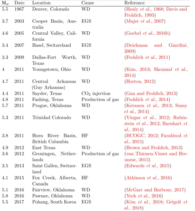
We conclude this section with a non exhaustive list of potentially induced earthquakes with magnitudes exceeding 3 (Table1.1).
We have presented so far a review of the major cases of induced seismicity. We will now discuss some common features between the different observations: (1) short or delayed time onset, (2) events spatial migration, (3) magnitude range of induced seismic sequences, (4) observed correlations with injection parameters, (5) and finally we will expose some observations regarding induced aseismic deformation and slip.
1.4.2 Temporal Correlation and Post Shut-in Seismicity
Variable time delays exist between the onset of induced seismicity and injection activity. For instance the seismic sequence near the Val d’Agri field in Italy initiated only 4 days after injection activity started (Valoroso et al., 2009; Stabile et al., 2014) and the one in Youngstown Ohio started 13 days after waste disposal activities started in the region (Kim, 2013). A very short time lag is also observed during hydraulic fracturing: 2 hours time lag in Ohio in 2013 (Kozlowska et al., 2018), as shown in Figure1.4.a for the induced seismicity in Harrison County, and 24 hours in California (Holland, 2013), or during geothermal operations (e.g. in Soultz-sous-ForêtMajer et al.(2007) andDorbath et al.
(2009) and Pohang Kim et al. (2018)). One reason behind the short time lag may be the high injection pressure. However, Kozlowska et al. (2018)argues that the seismicity triggered after 2 hours in Harrison County Ohio is faster than pressure diffusion and may be due to fast poro-elastic changes in pressure. On the other hand, a very long time lag is also observed in some cases, for example in the Codgell oil field in Texas the first event was recorded 18 years after injection activity started (Davis and Pennington, 1989). In this case, the pore pressure diffusion is expected to be very slow, mainly due to the existence of low permeability fluid baffles between the injection well and the neighbouring faults. This may lead the seismicity to occur even years after injection ends (Keranen and Weingarten, 2018).
Moreover, Schoenball et al. (2018)reported two temporal behaviors for the seismicity in Oklahoma and Southern Kansas for the different induced seismic sequences: one sequence was governed by a slow process, while another one was governed by a fast process. Post Shut-in Seismicity
Post shut-in seismicity is vastly observed for fluid injection activity. High seismic activity was recorded for nearly two years after injection stopped in Denver Colorado (Healy et al., 1968). Hsieh and Bredehoeft (1981) argued that pressure diffusion is the principal cause of post shut-in seismicity in this case because the fluid was injected into
Mw Date Location Cause Reference
5.5 1967 Denver, Colorado WD (Healy et al., 1968;Davis and
Frohlich, 1993) 3.7 2003 Cooper Basin,
Aus-tralia EGS (Majer et al., 2007)
4.6 2005 Central Valley,
Cali-fornia WD (Goebel et al., 2016b)
3.4 2007 Basel, Switzerland EGS (Deichman and Giardini,
2009) 3.3 2009 Dallas-Fort Worth,
Texas WD (Frohlich et al., 2011)
4 2011 Youngstown, Ohio WD (Kim, 2013; Skoumal et al.,
2014) 4.7 2011 Central Arkansas
(Guy Arkansas) WD (Horton, 2012)
4.4 2011 Snyder, Texas CO2 injection (Gan and Frohlich, 2013)
4.8 2011 Fashing, Texas Production of gas (Frohlich et al., 2014)
5.7 2011 Prague, Oklahoma WD (Keranen et al., 2013; Sumy
et al., 2014)
5.3 2011 Trinidad Colorado WD (Viegas et al., 2012;
Rubin-stein et al., 2012;Barnhart et
al., 2014)
3.8 2011 Horn River Basin,
British Columbia HF al.(BCOGC, 2012, 2015) ; Farahbod et
4.9 2012 East Texas WD (Brown and Frohlich, 2013)
3.6 2012 Groningen,
Nether-lands Production of gas (unese, 2015van Thienen-Visser and Bre-) 3.5 2013 Saint Gallen,
Switzer-land EGS (Edwards et al., 2015) 4.1 2015 Fox Creek, Alberta,
Canada HF (Atkinson et al., 2016)
5.1 2016 Fairview, Oklahoma WD (McGarr and Barbour, 2017)
5.8 2016 Pawnee, Oklahoma WD (Yeck et al., 2016)
5.5 2017 Pohang, South Korea EGS (Kim et al., 2018; Grigoli et
al., 2018)
1[Note. ]WD = Waste Disposal; EGS = Enhanced Geothermal Systems; HF = Hydraulic
Fracturing.
Table 1.1– List (non exhaustive) of potentially induced large earthquakes (Mw> 3) by fluid injection
1.4 Observations of Injection Induced Fault Reactivation
Figure 1.4 – Panel a: Map of hydraulic fracturing operations in Ohio where squares represent stimulation stages and circles represent induced seismicity. The time lag is represented by the color scale and shows how seismic activity starts very shortly following hydraulic operations, from (Kozlowska et al., 2018). Panel b: Time series of the pressure (red), flow rate (blue) and cumulative seismic moment (black for all earthquakes and violet for earthquakes with magnitude less than 2) during the stimulation in Soultz-sous-Forêt in 2000: seismic activity continues for several days after stimulation ends, from (Dorbath et al., 2009)
a fracture zone surrounded by low permeability cristalline basement. In Basel, several hours after the project shut down, a large ML 3.4 was recorded 3 kilometers under the
city (Deichman and Giardini, 2009) and micro-seismicity continued for two more years (Haring et al., 2008; Deichman and Giardini, 2009). Post shut-in seismicity was also recorded for several days at the EGS site in Soultz-sous-Forêt as shown in Figure1.4.b (Dorbath et al., 2009). Moreover, it was observed that for geothermal projects, the largest magnitudes tend to occur shortly after the end of injection (Langenbruch and Shapiro, 2010).
It is very difficult to assess whether or not seismicity will continue after shut-in, and what between reservoir or injection properties could dominate the post shut-in seismic activity (Majer et al., 2007). For instance,
• During the waste disposal activity in Youngstown Ohio in 2011, quiescence intervals were observed during short periods of no pumping at the wellhead during holidays. The observed quiescence period length decreased as the pressure at the wellhead and the injected volume increased. And after the final shut-in, where the pressure was at its highest (17 MPa), earthquakes continued at a smaller rate after shut-in with respect to during waste disposal activity (Kim, 2013).
This observation would suggest a correlation between shut-in seismicity and the injection pressure and injected volume. On the other hand,
• During hydraulic fracturing operation in the eastern part of Ohio in 2013, seismicity continued after shut-in for the deep seismic sequences, while it stopped for the shallow ones (Kozlowska et al., 2018).
• During waste disposal activity in Arkansas, after injection shut-in in 2016 seismicity stopped in the vicinity of the well, but continued at larger distances 10 km away (Rubinstein et al., 2018).
These observations in turn puts in evidence the effect of the reservoir parameters and permeability of the medium.
Finally, the characteristics of post-injection seismicity differ from one case to another. No systematic common observations were reported. As different parameters appear to influence post shut-in seismicity (injection pressure, volume, reservoir parameters and medium permeability), this issue remains to be further investigated and explored.
1.4.3 Spatial Migration of events
Spatial migration of events is commonly observed during injection induced seismic sequences (Rubinstein and Mahani, 2015). Earthquakes were recorded at least 10 km away from the injection well during the disposal of waste fluids in Denver, Colorado (Healy et al., 1968;Hermann et al., 1981;Hsieh and Bredehoeft, 1981). In Ohio,
earth-quakes migrated away from the well from the eastern part, close to the injection, of the fault to the western part (Kim, 2013). As for Oklahoma, earthquakes were recorded 20 km away from the well in 2014 (Keranen et al., 2014), and continued to migrate until seismicity spread over an area of 200 by 200 km2 (Schoenball and Ellsworth, 2017).
Figures 1.5a and 1.5b illustrate the migration of the seismic events away from the well at the Fenton Hill experiment in 1983 and the Soultz-sous-Forêt experiment in 1993, respectively, reported byShapiro et al. (1997,2002).
1.4 Observations of Injection Induced Fault Reactivation
Figure 1.5 – Time series of the distance of recorded events with respect to the injec-tion source for a) the Fenton Hill experiment in 1983 and b) the Soultz-sous-Forêt experiment in 1993, from (Shapiro et al., 1997)
1.4.4 Magnitude Content
The magnitude content of a seismic sequence is often represented through the b-value of the Gutenberg-Richter magnitude distribution (Gutenberg and Richter, 1954), where a decrease of the b-value could be interpreted by an increase in the frequency of large magnitudes and an increase of the b-value indicates an increase in the frequency of lower magnitudes. Low b-values were observed for several cases of injection induced seismicity: (1) a low b-value (< 1) was observed for the entire seismic sequence in Ohio (Skoumal
et al., 2014) as shown in Figure1.6.a; (2) a decrease in the b-value from 1.3 to 1.1 was
associated with fault reactivation due to fluid injection in Oklahoma (Goebel et al., 2016a) as shown in Figure1.6.b; (3) a strong decrease of the b-value from 1 to 0.6 accompanied a strong deviation of the magnitude distribution from typical Gutenberg-Richter behavior during injection for the earthquake swarm in California in 2005 (Goebel et al., 2016b) as shown in Figure 1.6.c; (4) and finally a decrease in the b-value was observed during hydraulic fracturing operations in Ohio in 2013 (Kozlowska et al., 2018). Schoenball
et al. (2015) argues that no change in the magnitude distribution was observed due
to the geothermal activities near the Coso field in California (Figure 1.6.d), however he compared recorded seismicity data near the geothermal field to the data recorded away from the field, both recorded during injection without knowledge of the magnitude distribution prior to injection activities.
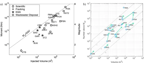
The magnitude content can also be characterized by the maximum magnitude of the events. Shapiro et al.(2007,2010,2011) argued that the size of the stimulated reservoir may control the size of the largest induced earthquake. However,McGarr (2014)proposed an upper bound limit to the seismic moment that depends especially of the total volume of fluid injected and showed that this limit is valid for the majority of injection induced seismicity cases (Figure 1.7.a). However, the recent 5.4 Pohang earthquake does not
Figure 1.6 – Panel a: Magnitude frequency distribution for induced seismicity in Young-stown Ohio, between 2011 and 2014, from (Skoumal et al., 2014). Panel b: Magnitude frequency distribution for induced seismicity in Oklahoma, between 1980 and 2008 in dark green and between 2009 and 2015 after seismic activity escalated in light green, from (Goebel et al., 2016a). Panel c: Magnitude frequency distribution for induced seismicity in California in 2005, before (green color), during (red color), and after (orange color) peak injection rates, from (Goebel et al., 2016b). Panel d: Magnitude frequency distribution: area B: 5 km radius area around the Coso geothermal field, area A-B: 30 km radius area from the geothermal field without area B, from (Schoenball
et al., 2015).
follow this estimation, as its real magnitude exceeds by two order the estimated one according to the associated injected volume in this case (Grigoli et al., 2018). On the other hand, according to Van der Elst et al. (2016), the maximum magnitude is not bounded by the injection volume, and can be as statistically expected. He argued that the injected volume controls the number of induced earthquakes exceeding a certain magnitude, rather than the maximum magnitude of the events as suggested by McGarr (2014) (Figure1.7.b).