Option Valuation with Conditional Skewness

Texte intégral

(1)2003s-50. Option Valuation with Conditional Skewness Peter Christoffersen, Steve Heston, Kris Jacobs. Série Scientifique Scientific Series. Montréal Août 2003. © 2003 Peter Christoffersen, Steve Heston, Kris Jacobs. Tous droits réservés. All rights reserved. Reproduction partielle permise avec citation du document source, incluant la notice ©. Short sections may be quoted without explicit permission, if full credit, including © notice, is given to the source..

(2) CIRANO Le CIRANO est un organisme sans but lucratif constitué en vertu de la Loi des compagnies du Québec. Le financement de son infrastructure et de ses activités de recherche provient des cotisations de ses organisationsmembres, d’une subvention d’infrastructure du ministère de la Recherche, de la Science et de la Technologie, de même que des subventions et mandats obtenus par ses équipes de recherche. CIRANO is a private non-profit organization incorporated under the Québec Companies Act. Its infrastructure and research activities are funded through fees paid by member organizations, an infrastructure grant from the Ministère de la Recherche, de la Science et de la Technologie, and grants and research mandates obtained by its research teams. Les organisations-partenaires / The Partner Organizations PARTENAIRE MAJEUR . Ministère du développement économique et régional [MDER] PARTENAIRES . Alcan inc. . Axa Canada . Banque du Canada . Banque Laurentienne du Canada . Banque Nationale du Canada . Banque Royale du Canada . Bell Canada . Bombardier . Bourse de Montréal . Développement des ressources humaines Canada [DRHC] . Fédération des caisses Desjardins du Québec . Gaz Métropolitain . Hydro-Québec . Industrie Canada . Ministère des Finances [MF] . Pratt & Whitney Canada Inc. . Raymond Chabot Grant Thornton . Ville de Montréal . École Polytechnique de Montréal . HEC Montréal . Université Concordia . Université de Montréal . Université du Québec à Montréal . Université Laval . Université McGill ASSOCIÉ À : . Institut de Finance Mathématique de Montréal (IFM 2) . Laboratoires universitaires Bell Canada . Réseau de calcul et de modélisation mathématique [RCM 2] . Réseau de centres d’excellence MITACS (Les mathématiques des technologies de l’information et des systèmes complexes) Les cahiers de la série scientifique (CS) visent à rendre accessibles des résultats de recherche effectuée au CIRANO afin de susciter échanges et commentaires. Ces cahiers sont écrits dans le style des publications scientifiques. Les idées et les opinions émises sont sous l’unique responsabilité des auteurs et ne représentent pas nécessairement les positions du CIRANO ou de ses partenaires. This paper presents research carried out at CIRANO and aims at encouraging discussion and comment. The observations and viewpoints expressed are the sole responsibility of the authors. They do not necessarily represent positions of CIRANO or its partners.. ISSN 1198-8177.

(3) Option Valuation with Conditional Skewness* Peter Christoffersen†, Steve Heston‡, Kris Jacobs§. Résumé / Abstract Il est clair empiriquement que les prix d'options sur indices diffèrent de manière systématique des prix Black-Scholes. Les prix des options de vente hors du cours (et les prix des options d'achat dans le cours) sont relativement élevés par rapport au prix Black-Scholes. Motivés par ces faits empiriques, nous développons un nouveau modèle dynamique à temps discret de rendements d'actions avec des innovations gaussiennes inverses. Le modèle permet de tenir compte de l'asymétrie conditionnelle ainsi que de l'hétéroskédasticité conditionnelle et d'un effet de levier financier. Nous présentons une formule analytique de prix d'option conforme à cette dynamique des rendements. Un test empirique intensif du modèle à partir des options sur l'indice S&P500 montre que la performance du nouveau modèle GARCH gaussien inverse est supérieure à celle des modèles imbriqués standards pour les options de vente hors du cours, de ce fait démontrant l'importance de l'asymétrie conditionnelle. Le processus GARCH gaussien inverse à temps discret présente deux limites intéressantes en temps continu. Une de ces limites correspond au modèle de volatilité stochastique standard de Heston (1993). L'autre est un processus de sauts purs avec intensité stochastique. En utilisant ces résultats de limites, une motivation équivalente pour notre modèle est qu'il généralise les modèles de volatilité stochastique standards de volatilité en permettant des "sauts" et d'autres mouvements négatifs de queues épaisses dans les rendements d'action. Les résultats empiriques démontrent donc également l'importance des sauts pour l'évaluation des prix d'options de vente hors du cours. Mots clés : GARCH, hors échantillon, sauts, modèles à temps discret, limites en temps continu.. There is extensive empirical evidence that index option prices systematically differ from Black-Scholes prices. Out-of-the- money put prices (and in-the- money call prices) are relatively high compared to the Black-Scholes price. Motivated by these empirical facts, we develop a new discrete time dynamic model of stock returns with Inverse Gaussian innovations. The model allows for conditional skewness as well as conditional *. We would like to thank Peter Carr, Frank Diebold, Rob Engle, Nour Meddahi and Haluk Unal for helpful comments. Christoffersen and Jacobs would like to thank FCAR, SSHRC and IFM2 for financial support. John Kozlowski provided expert research assistance. Any remaining errors are ours. † Faculty of Management, McGill University and CIRANO, Montreal, Quebec, H3A 1G5, Canada, email: [email protected]. ‡ Corresponding author. R.H. Smith School of Business, University of Maryland, College Park, MD 20742, email: [email protected]. § Faculty of Management, McGill University and CIRANO, Montreal, Quebec, H3A 1G5, Canada, email: [email protected]..

(4) heteroskedasticity and a leverage effect. We present an analytic option pricing formula consistent with this stock return dynamic. An extensive empirical test of the model using S&P500 index options shows that the new Inverse Gaussian GARCH model’s performance is superior to a standard existing nested model for out-of-the money puts, thus demonstrating the importance of conditional skewness. The discrete-time Inverse Gaussian GARCH process has two interesting continuous-time limits. One limit is the standard stochastic volatility model of Heston (1993). The other is a pure jump process with stochastic intensity. Using these limit results, an equivalent motivation for our model is that it generalizes standard stochastic volatility models by allowing for “jumps” and other fat-tailed negative movements in stock returns. The empirical results therefore also demonstrate the importance of jumps for the pricing of out-of-the-money puts. Keywords: GARCH, out-of-sample, jumps, discrete-time model, continuoustime limit. Codes JEL : G12.

(5) Introduction There is extensive empirical evidence that index option prices systematically differ from the Black-Scholes formula.1 Out-of-the-money put prices (and in-the-money call prices) are relatively high compared to the Black-Scholes price. This stylized fact is often represented by the well-known “volatility smirk”. One interesting approach to capturing these deviations from the Black-Scholes formula is to incorporate models of conditional heteroskedasticity (Hull and White (1987), Scott (1987), Heston (1993)). At the empirical level, a number of papers have demonstrated that these models significantly improve upon the performance of the Black-Scholes model (e.g., see Bakshi, Cao, and Chen (1997), Bates (2000), Ding and Granger (1996), Engle and Mustafa (1992), Jones (2003) and Pan (2002)). Moreover, several papers have demonstrated that the performance of option valuation models with conditional heteroskedasticity can be further improved by including a so-called leverage parameter (Nandi (1998), Heston and Nandi (2000), Chernov and Ghysels (2000), Christoffersen and Jacobs (2002)). The combination of leverage parameters and stochastic volatility or conditional heteroskedasticity captures the stylized fact that volatility increases relatively more when the stock price drops (Black (1976), Christie (1982)). This increases the probability of a large loss and consequently the value of out-of-the-money put options. Equivalently, the implications of the leverage effect can be understood by realizing that it generates negative skewness in stock returns.2 While stochastic volatility models are intuitively and theoretically appealing, they may not be sufficient to explain observed option biases, even with leverage parameters included. This is particularly the case for options with short maturities. While the leverage parameter creates negative See for example Ait-Sahalia and Lo (1998), Bakshi, Cao, Chen, (1997), Bates (1996), Christoffersen and Jacobs (2002), Das and Sundaram (1999), Dumas, Fleming, and Whaley (1998) and Jackwerth (2000). 1. 2. See Heston (1993) for an in-depth analysis of the impact of the leverage parameter on option prices.. 2.

(6) skewness in multi-period returns, single-period innovations are Gaussian in these models, and therefore standard models cannot explain the strong biases in short-term options. A complementary approach to generate skewness in the return distribution is to model the conditional innovations to returns using a distribution with nonzero third moment. This paper develops a model for spot prices that introduces conditional skewness into shortterm spot returns in addition to conditional heteroskedasticity and a leverage effect. We model the conditional return innovation using an Inverse Gaussian distribution, and we combine the modeling of these nonstandard conditional innovations with a fairly standard model of time-varying conditional volatility that also contains a leverage effect. The resulting return dynamic, which we call Inverse Gaussian GARCH, is able to capture skewness in short-term as well as long-term returns, and the conditional skewness reinforces the effects of the leverage parameter. We present a closed-form option pricing formula consistent with this return dynamic. The discrete-time Inverse Gaussian GARCH process has two interesting continuous-time limits. One limit is the standard stochastic volatility model of Heston (1993). The other is a pure jump process with stochastic intensity. Using these limit results, an equivalent motivation for our model is therefore that it generalizes standard stochastic volatility models by allowing for “jumps” and other fat-tailed negative movements in short-term stock returns, which is particularly useful for explaining the biases in short-term options (Carr and Wu (2003)). However, while jumps in stock returns reduce the bias in option prices, they cannot adequately address the magnitude of this bias (Bates (1996)). In other words, introducing jumps in returns works in a qualitative sense, because it reduces the biases, but not in a quantitative sense, because part of the bias remains. We therefore need a modeling approach that reinforces the effects of jumps in returns. One of the continuous-time limits of our model additionally contains jumps in volatility, and allows these jumps to be (negatively) correlated with jumps in stock returns (see also Duffie, Pan and Singleton (2000), Pan (2002), Eraker (2003), Eraker, Johannes and Polson (2002), and Duan, Ritchken and Sun (2002)). Compared to jumps in returns, jumps in volatility can have a larger impact on option prices because the volatility process is 3.

(7) very persistent whereas the return process is not. With jumps in volatility, a series of moderate negative “jumps” in stock returns can dramatically increase volatility for a prolonged period. Small changes in the distribution of stock returns can therefore have a potentially large impact on option values. We implement the model empirically using data on S&P500 index options. We compare the model’s performance to the Black-Scholes model as well as to a number of benchmarks. We find that our model performs well compared to these benchmarks. The most relevant benchmark for our model is the Heston-Nandi (2000) model, which is a model with conditional heteroskedasticity, a leverage effect and Gaussian innovations, and which is nested in our model. In-sample the Inverse Gaussian model improves upon the performance of the Heston-Nandi model in every respect, which is not surprising because it nests the Heston-Nandi model. Out-of-sample, the model’s performance is mixed. While the Inverse Gaussian model improves on the Heston-Nandi model for the valuation of out-of-the-money puts, this is not necessarily the case for other options. When keeping the model parameters constant for up to ten weeks, the valuation of the Inverse Gaussian model improves on that of the Heston-Nandi model. However, when keeping the parameter estimates constant for longer periods, the Inverse Gaussian model is outperformed by the Heston-Nandi model. We therefore conclude that the benefits of modeling conditional skewness and jump processes are mixed, and depend on the use of the models; the richer parameterization of these models is helpful in-sample and for some out-of-sample assessments, but a more parsimonious parameterization may be preferable dependent on the strategy one pursues. Presumably many strategies that use options only rely on keeping the parameters constant for short periods out-of-sample, even though changing the model parameters implies a theoretical inconsistency. The model is presented in the next two sections. Subsequently we present empirical assessments of the model using S&P500 index returns and options prices. A final section concludes and discusses directions for future research. Some technical material on the Inverse Gaussian distribution is relegated to the appendix. 4.

(8) 1. The Stock Price Dynamics 1.1. The Inverse Gaussian Process The basic building block for this model is an Inverse Gaussian innovation. The Inverse Gaussian distribution characterizes a stochastic process y defined by independent increments over disjoint intervals where q(t)-q(s) follows an Inverse Gamma process with degrees of freedom δ(t-s). By subtracting the drift, the process q(t)-δt is a martingale. This “random walk” takes an infinite number of jumps in every interval, but most of those jumps are very small. The degrees of freedom parameter δ determines the overall intensity or frequency of these jumps. As δ approaches infinity the normalized Inverse Gaussian process converges to a Wiener process.3 The Inverse Gaussian distribution function with parameter δ is given by x ⌠ P(x;δ) = ⌡ 0. δ. -δ -δ e-( z-δ/ z)2/2dz = N( + x) + e2δN( - x). x x 2πz3. (1). Straightforward (albeit tedious) integration gives the moment generating function: E[exp(φy+θ/y)] =. δ exp(δ- (δ2-2θ)(1-2φ)). 2 δ -2θ. (2). and the moments: E[y] = δ, Var[y] = δ,. (3). E[1/y] = 1/δ + 1/δ2, Var[1/y] = 1/δ3+ 2δ4, Skew[y] = 3/Sqrt(δ), Cov[y,1/y] = -1/δ.. For more detail see Johnson, Kotz and Balakrishnan (1994), chapter 15. For an intuitive derivation of the inverse Gaussian distribution see Whitmore and Seshadri (1987). 3. 5.

(9) 1.2. The Inverse Gaussian GARCH Process We combine the conditional skewness of the Inverse Gaussian distribution with GARCH-type dynamics that contain conditional heteroskedasticity and a leverage effect.4 This gives the model flexibility to capture moneyness effects for short-term as well as long-term options. The new dynamic model specifies returns on a spot asset price at time t, S(t+∆), and the conditional variance h(t+∆) as log(S(t+∆)/(S(t)) = r + νh(t+∆) + ηy(t+∆),. (4a). h(t+∆) = w + bh(t) + cy(t) + ah(t)2/y(t),. (4b). where y(t) has an Inverse Gaussian distribution with degrees of freedom parameter δ(t) = h(t)/η2. If η is negative then stock returns display negative conditional skewness as illustrated in Figure 1. We label this model the Inverse Gaussian GARCH(1,1), because it consists of combining an Inverse Gaussian distribution with a GARCH(1,1) type volatility dynamic in (4b).5 We can use the moments of the Inverse Gaussian in (3) to show the conditional mean and variance of the spot process (4) are linear functions of the current variance. From equation (4a) the conditional mean and variance can be derived as Et[log(S(t+∆)/S(t))] = r + (ν+η-1)h(t+∆),. (5a). Vart[log(S(t+∆))] = h(t+∆). And from equation (4b) we can compute variance persistence as the coefficient on h(t+∆) in Et[h(t+2∆)] = w + η4a + (aη2+b+c/η2)h(t+∆),. (5b). It can also be seen from (5b) that the unconditional variance is (w + η4a)/(aη2+b+c/η2). See Nelson (1991) for another approach that alters the GARCH dynamic and introduces conditional nonnormality. 5 For more complex dynamics one can nest higher-order GARCH processes by adding lagged disturbances to the dynamics of the conditional variance. 4. 6.

(10) The variance of variance is given from equation (4b) by Vart[h(t+2∆)] = 2a2η8+(c2/η2-2η2ac+a2η6)h(t+∆),. (5c). And the leverage effect can be quantified as the conditional covariance between returns and variance as in Covt[log(S(t+∆),h(t+2∆)] = (c/η-η3a)h(t+∆).. (5d). Although the functional form appears quite different, the Inverse Gaussian GARCH is closely related to previous GARCH processes. By taking the limit as η approaches zero and using the following parameterization, ν = λ-η-1, w = ω, a = α/η4,. (6). b = β + αγ2-2α/η2+2αγ/η, c = α-2ηαγ. the inverse Gaussian GARCH(1,1) converges to the Heston-Nandi (2000) asymmetric GARCH model with normal disturbances z(t+∆) log(S(t+∆)/S(t)) = r + λh(t+∆) + h(t+∆)z(t+∆),. (7a). h(t+∆) = ω + βh(t)+ α(z(t)-γ h(t))2.. (7b). The parameterization in (6) matches the first two conditional moments of the Inverse Gaussian GARCH model with those in the Heston-Nandi model. Additionally by letting η approach zero, the skewness disappears and the Inverse Gaussian model converges to the Heston-Nandi model in distribution. 1.3. Continuous-Time Limits While the Inverse Gaussian GARCH(1,1) is a discrete model that is readily implementable with discrete data, it has two interesting continuous-time limits. First, when η approach zero, it. 7.

(11) converges to Heston’s (1993) square-root model as a diffusion limit.6 Consider letting the time interval ∆ shrink to zero and define v(t) = h(t)/∆ to be the variance per unit of time. Then let ω(∆) = (κθ-¼σ2)∆2, β = 0, α(∆) = ¼σ2∆2, γ(∆) = 2/(σ∆)-κ/σ. As the time interval shrinks the variance per unit of time converges weakly to the square-root diffusion process dv(t) = κ(θ-v(t)) + σ v(t)dz,. (8). where z(t) is a Wiener process. Second, we can let the time interval shrink with the alternative parameter limits r(∆) = r∆, a(∆) = 0, b(∆) = 1-b∆,. (9). c(∆) = c∆, w(∆) = w∆2. Again letting v(t) = h(t)/∆ represent the variance per unit of time we obtain a pure jump process as the time interval shrinks d(log(S(t))) = (r+νv(t)))dt + ηdy(t),. (10a). dv(t) = (w-bv(t))dt + c dy(t),. (10b). where y(t) is a pure-jump inverse Gaussian process with degrees of freedom δ(t) = v(t)/η2 in the interval [t,t+dt]. The stock price converges to a pure jump process with stochastic intensity. The Inverse Gaussian process has also been investigated by Barndorff-Nielsen and Levendorskii (2000).7 To provide some more intuition for the dynamics of this process, Figure 2 shows how an Inverse Gaussian random walk converges to a Wiener process as the skewness parameter converges to zero. In summary, the continuous-time limits suggest that the dynamic process (4) displays remarkable flexibility: it is able to capture both diffusion processes and pure jump processes dependent on the degree of skewness or kurtosis of returns. 6 7. See Nelson (1990) and Heston and Nandi (2000). See also the excellent overview of related processes in Barndorff-Nielsen and Shephard (2001). 8.

(12) 2. Option Valuation Option valuation in the Inverse Gaussian GARCH model requires additional assumptions. In the limiting diffusion case the stock return completely spans uncertainty in variance. Consequently one can uniquely value options through the absence of arbitrage. But in the limiting jump case this is not possible.8. Consequently we make an assumption that has become standard in discrete. implementations of option models (Amin and Ng (1993), Duan (1995), Duan, Ritchken and Sun (2002), Heston and Nandi (2000) and Stutzer (1996)). This assumption ensures the distribution of spot returns remains Inverse Gaussian GARCH under the risk-neutral valuation probability measure. Assumption:. There is a local Risk Neutral Valuation Relationship.. The resulting risk-neutral distribution of returns is Inverse Gaussian GARCH, but with a different parameterization.9. There are two equivalent ways of characterizing the risk-neutral. dynamics. The first characterization is useful to mechanically understand the transformation from the true dynamic in (4) to the risk neutral dynamic. Appendix B shows that given the local Risk Neutral Valuation Relationship, the risk-neutral parameters are η* = ν2η3/(1+ ½ν2η3)2,. (11). δ*(t) = δ(t) η/η*. We can then use δ(t) = h(t)/η2 and δ∗(t) = h*(t)/η2 to derive h*(t) = h(t)(η*/η)3/2. Substituting this expression and the risk-neutral parameters (11) into the original process (4) allows us to characterize the risk-neutral dynamics as an Inverse Gaussian GARCH process. Proposition 1: Under the risk neutral probabilities the stock price follows the process With an Inverse Gaussian process the stock price can instantanteously jump to an infinite number of values. This cannot be represented as a binary process. Basically if one weakens the assumptions about the distribution of returns then one must strengthen the assumptions about valuation. 9 Gerber and Shiu (1993, 1994) developed a three-parameter option valuation formula using the Inverse Gaussian distribution. 8. 9.

(13) log(S(t+∆)) = log(S(t)) + r + ν*h*(t+∆) + η*y*(t+∆), h*(t+∆) = w* + bh*(t) + c*y*(t) + a* h*(t)2/y*(t),. (12a) (12b). where ν* = ν(η*/η)-3/2, y*(t) = y(t)(η*/η)-1, w* = w(η*/η)3/2, c* = c(η*/η)5/2, a* = a(η*/η)-5/2, and y*(t) has an Inverse Gaussian distribution with parameter δ*(t) = h*(t)/η*2. The risk-neutral dynamic in (12) contains six parameters ν*, w*, b, c*, a* and η*. Appendix C characterizes the risk-neutral dynamic in a different but equivalent way, which clarifies that in fact η* is a function of the other parameters. The risk-neutral dynamic therefore only contains five independent parameters. This is analogous to the Black-Scholes formula where the true drift parameter of the stock price is eliminated from the (risk-neutral) pricing formula. In our model option values depend only on the history of the stock price, as summarized by the conditional volatility, and on the five risk-neutral parameters ν*, w*, b, c*, and a*. To provide some intuition for the pricing in this model, consider the discounted expected payoff, which yields a simple two-parameter generalization of the Black-Scholes (1973) formula. Proposition 2: The value of a one-day call option with strike price K is ln(K / S) − r − ν * v * ** ln(K / S) − r − ν * v * * ; δ ) - Ke-rP( ; δ ), for η < 0, η ** η*. (13a). ln(K / S) − r − ν * v * ** ln(K / S) − r − ν * v * * ; δ )] - Ke-r[1-P( ; δ )], for η > 0, η** η*. (13b). C = S P( and C = S [1-P(. where η** = η*/(1-2η*) and δ** = δ* 1−2η*.. 10.

(14) and where P(.) represents the Inverse Gaussian distribution function. The formula converges to the Black-Scholes formula as the degrees of freedom parameter δ gets large, which is not surprising given the convergence result for the Inverse Gaussian distribution. Given the risk-neutral probability distribution and characteristic function (see Appendix A), we can value a call option using the inversion formula of Heston and Nandi (2000) or Bakshi and Madan (2000). This “closed-form” solution is very convenient in empirical work. It avoids the use of numerical methods or Monte Carlo techniques, which in many applications are potentially slower and less accurate. Proposition 3: At time t, a European call option with strike price K that expires at time T is worth C = e-r(T-t)Et∗[Max(S(T)-K,0)] =. (14). ∞ ∞ -iφ ∗ -r(T-t) ⌠ K f (iφ+1) e 1 ⌠ K-iφf∗(iφ) Re[ S(t)(½ + ]dφ) – Ke-r(T-t)(½ + Re[ ]dφ), iφ iφ π ⌡ π⌡ 0 0 where f*(iφ) denotes the characteristic function of the risk-neutral process given in the appendix. Figure 3 provides some intuition for the potential benefits of the Inverse Gaussian GARCH model. All pictures represent the price of European call options with an exercise price of $100 and have the value of the current stock price on the horizontal axis. The two top pictures show the difference between either the Heston-Nandi and Black-Scholes prices or the Inverted Gaussian GARCH and Black-Scholes prices, for an option with twenty days to maturity (in dollars). It can be seen that both the Heston-Nandi and Inverted Gaussian GARCH models lower the price of out-of-themoney calls and increase the price of in-the-money calls vis-à-vis the Black-Scholes model. The effect is stronger for the Inverted Gaussian GARCH, and is also stronger the more negative the skewness parameter η*. To provide some more perspective for these results, note that the BlackScholes price is $0.54 when the current stock price is $95. It can be seen from Figure 3 that the. 11.

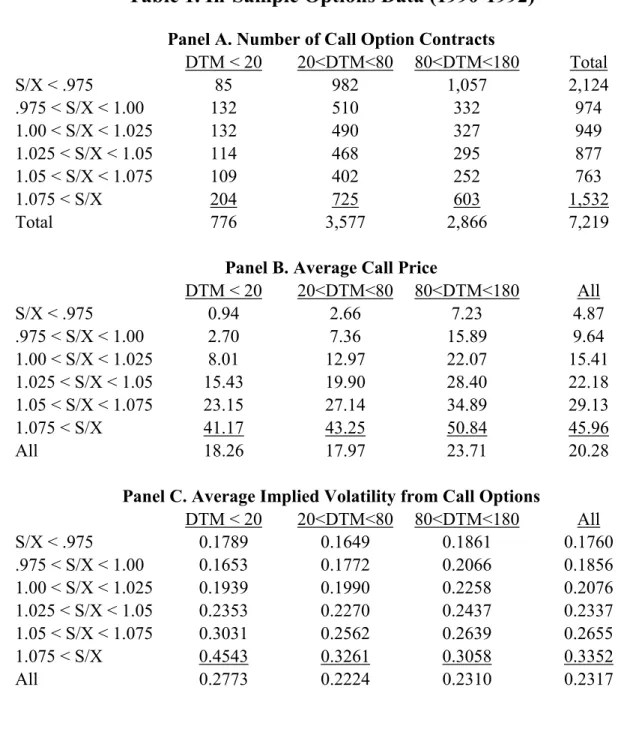
(15) difference in prices between the IG GARCH and Black-Scholes model is more than ten cents, which is substantial on a 54 cent option. The bottom two pictures present results for the difference between the IG and HN models. The interesting observation is that the maximum dollar effect of the IG GARCH model does not differ much by maturity, but that the maturity slightly affects at which moneyness the model has maximum impact. 3. Empirical Results 3.1. Options Data We now turn to the empirical results on the Inverse Gaussian GARCH model (henceforth referred to as IG GARCH). We also provide empirical results on the Heston and Nandi (2000) model (HN), which is nested in the IG GARCH model and therefore provides an interesting benchmark. We implement these models using a data set on S&P500 European call options (SPX) from the CBOE. The liquidity in the SPX option market is relatively high, and this market has therefore been analyzed by a number of researchers.10 We split up our data into an in-sample and an out-of-sample period; the models are estimated using the in-sample data only. Table 1 gives an overview of the in-sample data, which consist of option contracts on 156 Wednesdays in the period January 2, 1990 through December 31, 1992.11 We restrict attention to option contracts with maturities between 7 and 180 days and we apply a number of standard filters to the data.12 The resulting in-sample data set consists of 7,219 Wednesday closing quotes. The average call option price for the entire sample is $20.28 and the average implied BlackScholes volatility is 23.17%. The well-known post-1987 volatility smirk is evident from Table 1C. The deep in-the-money call option implied volatility is more than 45% for options with less than 20 See for example Bakshi, Cao and Chen (1997), Chernov and Ghysels (2000), Dumas, Fleming and Whaley (1998), Heston and Nandi (2000) and the references therein. 11 We use Wednesdays only to keep the computations manageable. The same approach was taken by Dumas, Fleming and Whaley (1998), Heston and Nandi (2000) and Christoffersen and Jacobs (2002). 12 We use the same filters as Bakshi, Cao and Chen (1997). 10. 12.

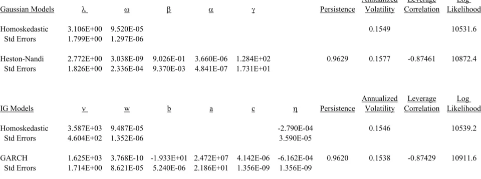
(16) days to maturity compared with less than 18% for the corresponding out-of-the-money call options. The smirk does flatten somewhat with maturity; for options with more than 80 days to maturity the implied volatility is more than 30% for deep in-the-money calls and less than 19% for out-of-themoney calls.. 3.2 Estimating the Models from Returns Under the True Statistical Probability Distribution Because the HN and IG GARCH option valuation models are derived starting from the return dynamics, differences between the models’ ability to price options should also be apparent from their ability to fit the dynamics of the underlying asset. In this section we compare the models’ ability to fit the returns on the underlying S&P500 index. In addition to the HN and IG GARCH valuation models, we also present estimation results on two nested models, which we label the homoskedastic Gaussian and the homoskedastic IG model, respectively. These models eliminate the GARCH effects from the dynamics in (4) and (7) by imposing β = α = γ = 0 and b = a = c = 0 respectively. The resulting homoskedastic models are two- and three-parameter models. A comparison of the fit of these two models indicates the importance of conditional skewness in the absence of heteroskedasticity and volatility clustering. Table 2 contains the Maximum Likelihood point estimates of the parameters for the Gaussian and IG models as well as their standard errors, obtained under the true statistical probability distribution.13 The models are estimated on daily total index returns from CRSP for the period January 3, 1989 through December 20, 2001. We use a time series that is longer than the option dataset because it is well known that it is difficult to estimate return dynamics precisely using short time series. Perhaps more interesting than the individual parameter estimates are the model properties reported in the bottom panel of Table 2. All models imply an unconditional volatility of approximately. The standard errors are calculated from the outer product of the vector of gradients evaluated at the ML parameter values. 13. 13.

(17) 15% per year. The HN model parameter estimates as well as the IG GARCH estimates imply a daily variance persistence of approximately 0.962. The leverage correlation is computed using the unconditional version of the moments in (5), specifically we compute the correlation as Cov[log(S(t+∆),h(t+2∆)] / { Stdev[log(S(t+∆))] * Stdev[h(t+2∆)] }. Notice that the leverage correlations are quite similar across models and are negative and quite large. The log-likelihoods allow several interesting tests. First, it is clear that in the Gaussian case the improvement in fit from the two-parameter homoskedastic model to the five parameter HN model is statistically significant at conventional significance levels. The same is true for the improvement in fit of the six-parameter IG GARCH model over the three-parameter homoskedastic IG model. Second, while the HN and IG GARCH models appear to be fairly similar in terms of the above characteristics, their log-likelihoods are dramatically different. The IG model has one extra parameter and provides a much better fit. The increase of over 39 points in log-likelihood going from the HN to the IG model is very large and statistically significant at conventional significance levels. The S&P500 return data thus strongly favor the IG specification. Third, the homoskedastic IG model improves on the fit of the homoskedastic Gaussian model and the extra parameter is significantly estimated. The increase of 7.6 in the log-likelihood is significant at conventional significance levels.. 3.3 Estimating the Risk Neutral Models Using Option Prices While the return-based estimation in Table 2 is interesting, it is well known that for the purpose of option valuation, parameters estimated from option prices are preferable to parameters estimated from the underlying returns (see for instance Chernov and Ghysels (2000)). We therefore estimate the HN and IG models using option prices. The implementation of these dynamic models is important and deserves comment. First consider the implementation of the Heston and Nandi (2000) model in (7), which has the risk-neutral dynamic. 14.

(18) log(S(t+∆)) = log(S(t)) + r – 0.5h∗(t+∆) +. h * ( t + 1) z*(t+∆),. h∗(t+∆) = ω + βh∗(t)+ α(z*(t)-γ∗ h * ( t ) )2,. (15a) (15b). Substituting (15b) in (15a) we get conditional variance in terms of observed returns h∗(t+∆) = ω + βh∗(t)+ (α/ h∗(t))( log(S(t)/S(t-∆)) - r + 0.5h∗(t) - γ∗h∗(t))2,. (16). The model is implemented by initializing h(0) using the unconditional variance (ω+α)/(1−β−αγ∗2) and then using the GARCH updating in (16). We start the iteration 250 trading days before the first option date to allow for the model to find the right conditional variance. In all experiments we set r equal to 0.05/365 (in our use of the dynamic in (16), not for pricing options). We then obtain estimates of the (risk-neutral) parameters ω, α, β and γ∗ by minimizing the mean squared error based on the difference between actual option prices and model values using NLS. MSE =. 1 N (C i,t − C i,t (ω, α, β, γ*))2 ∑ N i,t. Now consider the IG model in (4) with its risk-neutral dynamic (12). Substituting (12b) in (12a) yields. h*(t+1) = w* + b h(t)* + (c*/σ*) (log(S(t+1)/S(t))-r - ν*h(t)*) + (a* h(t)*2σ*) / (log(S(t+1)/S(t)) – r - ν*h(t)* ). (17). Again, we initialize h*(0) using the unconditional variance (w*+σ*4 a*)/(1− a ∗σ*2−b*− c*/σ*2) and then we use the GARCH updating rule. Minimizing the dollar-based mean squared error gives us estimates of the five independent parameters w*, σ*, a ∗, b* and c*. It must be noted that the updating rules (16) and (17) will also be used in the out-of-sample analysis below. The discrete-time GARCH formula enables daily valuation of out-of-sample option values in a straightforward way, which is a strength of this type of model.. 15.

(19) Table 3 shows the nonlinear least squares (NLS) estimates of the four models analyzed in Table 2, obtained by minimizing the squared dollar option pricing error, using data for 156 Wednesdays in the 1990-1992 period. Panel A shows the estimates using all the 7,219 option contracts in the sample whereas Panel B only uses the 776 options with at most 20 days to maturity. The parameter estimates in Table 3 refer to the risk neutral representation of the models. Note that all four models contain one less parameter compared to their representation under the true statistical distribution in Table 2. As demonstrated by Heston and Nandi (2000), the HN model performs quite well in valuing SPX options. The root mean squared error (RMSE) for the 7,219 contracts with an average price of $20.28 (Table 1.B) is $1.0043 for the HN model. The IG GARCH model performs slightly better with an RMSE of $0.9586, which represents a 4.77% improvement. When estimating the models on the short-term contracts, the RMSE is of course lower for both models. The RMSE for the HN model is now $0.6072 versus $0.5702 for the IG model, which represents a 6.5% improvement. The relative improvement in fit resulting from the extra parameter in the IG specification is thus larger for shorter-maturity options. Table 3 allows for a number of other conclusions from comparing the four models as well as from a comparison with the results in Table 2. First, the improvement in fit resulting from adding three extra parameters in the GARCH models vis-à-vis the homoskedastic models is always substantial, but the improvement is smaller in Panel B. Second, the improvement in fit resulting from one extra parameter in the IG models is larger for the homoskedastic models. Perhaps related to this, the estimate of η* is much larger (in absolute value) for the homoskedastic model. Third, the leverage correlation is close to –1 in all cases, and is much larger (in absolute value) than the leverage correlation for the true statistical distribution documented in Table 2. Fourth, for the GARCH models the persistence of the variance is higher under the risk neutral than under the true statistical representation in Table 2. This is true when estimating the models using all maturities, and also when restricting the sample to maturities of at most 20 days. While Table 3 only reports the aggregate fit of the two GARCH models, Table 4 shows the fit in mean squared error across maturity and moneyness bins. Table 4 uses the parameter estimates based 16.

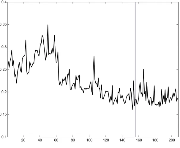
(20) on all the available contracts. Note that generally the dollar fit is better for the cheaper short-term (left column) and out-of-the-money call options (top rows). A comparison of the two models is most easily done using Table 4C which reports the ratio of the MSEs of the two models. The bottom row (marked “All”) indicates that the IG model outperforms the HN model for all three maturity bins but mostly so for the longer-term options. The rightmost column (also marked “All”) indicates that the IG model outperforms the HN model for all moneyness bins. Most of the improvement comes from the out-ofthe-money calls, and to some degree from the deep in-the-money calls, which from put-call parity correspond to deep out-of-the-money puts. Table 5 provides additional evidence on these improvements in fit. Each panel presents model bias, which is defined as market price minus model price, across moneyness and maturities. Panel C indicates that the Black-Scholes price is too high for deep out-of-the-money calls and too low for deep in-the-money calls. Figure 3 suggests that the HN and IG GARCH models can potentially address these biases, and Table 5 confirms that this is indeed the case for these data. The Black-Scholes biases have the same sign but are much smaller in absolute value in Panel A for the HN model, and smaller yet in Panel B for the IG GARCH model. Interestingly, however, most biases are still present with the same sign.. 3.4. Out-of-Sample Analysis The true test of any estimated model is its out-of-sample performance. We therefore evaluate the models’ performance using option data on 52 additional Wednesdays corresponding to the 1993 calendar year.14 We apply the same filters to these data and again restrict attention to options with maturities between 7 and 180 days. The basic features of the 2,985 contracts in the out-of-sample data set are reported across maturity and moneyness bins in Table 6. Notice again the steep smirk for shortterm options. Figure 4 graphs the average implied volatility for the 208 Wednesdays in the in-sample When calcuating option values out-of-sample, we update information on interest rates and stock index values but we use the parameters from the in-sample estimation period. For details on the outof-sample implementation in this type of discrete time models, see Heston and Nandi (2000) and Christoffersen and Jacobs (2002). 14. 17.

(21) and the out-of-sample period. It is clear that the data display substantial volatility clustering and that there are substantial changes in implied volatility over the four-year period. For the interpretation of the out-of-sample results, it is important to note that the implied volatility in the out-of-sample period is lower than in the in-sample period, and that volatility seems to have been trending downward over the period 1990-1993. Table 7 shows the overall out-of-sample MSE for the HN and IG models during the out-ofsample period. Each model is evaluated using the parameter estimates from the 1990-1992 sample period. Notice that overall the more parsimonious HN model performs much better than the IG model out-of-sample. This conclusion holds when all options are included (Panel A) but also when the sample is limited to options with less than 20 days to maturity (Panel B). It is also interesting that in Panel A the deterioration in the HN model going from in-sample to out-of-sample is minor, whereas the deterioration in the IG model is substantial.. 3.6. Interpretation Table 7 suggests that the IG GARCH model performs poorly out-of-sample. However, Table 8 and Figures 5 and 6 show that one has to be cautious when investigating the out-of-sample performance of the IG GARCH model. Table 8 analyzes the out-of-sample performance of the HN and the IG GARCH model by maturity and moneyness. Table 8C shows the ratio of the IG to HN model MSEs. Considering the rightmost column we see that the out-of-sample performance of the IG model is particularly poor for the longer-term options. Considering the bottom row we see that the IG model is actually better than the HN model for the deep in-the-money call options. Whereas the in-sample results in Table 4 showed improvements in IG over HN for both in-the-money and out-of-the-money options the conditional skewness in the IG model only has an beneficial effect out-of-sample for the deepest in-the-money calls (and equivalently the deepest out-of-the-money puts). We therefore conclude that the out-of-sample performance of the IG GARCH model is satisfactory for addressing one important remaining problem in option valuation, the valuation of out-of-the-money puts. However, the model fails out-of-sample along a number of other dimensions. 18.

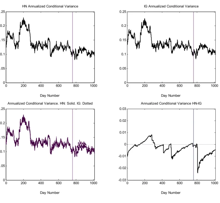
(22) Figure 5 shows the cumulative RMSEs as a function of time in the in- and out-of-sample periods. The top left panel of Figure 5 shows the cumulative in-sample RMSEs for the two models. Both models have relatively stable RMSEs over time and the RMSE for the IG model (solid line) tends to be below or very close to the HN model (dashed). The bottom left panel reports the ratio of the cumulative in-sample RMSEs. It appears that the IG model improvements come from early in the sample as well as around week number 100. The full in-sample RMSE ratio is .9586/1.0043 = .9545. More interesting are the corresponding figures for the 52-week out-of-sample period. The top right panel shows the cumulative RMSE for the two models and the bottom panel shows the ratio of the RMSEs. It is quite striking how the in-sample improvement in IG over HN continues 10 weeks into the out-of-sample period. Beyond 10 weeks out-of-sample, both models deteriorate substantially; however, the performance of the IG model deteriorates much more than that of the HN model. Consequently, the ratio of the RMSEs increases sharply from week 10 through week 25 until it reaches its full out-of-sample average of 1.3611/1.0778 = 1.2629. One possible interpretation of these findings is that the conditional skewness parameter η* in the IG model is difficult to estimate perhaps because it is truly dynamic. Keeping the IG parameters constant over long periods in an out-of-sample analysis puts heavy demands on the models and causes its performance to deteriorate. More generally, it must of course be noted that this type of long out-of-sample valuation exercise may simply be too ambitious for this type of models, as may be evidenced by the deteriorating RMSE as a function of the forecast horizon. Figure 6 repeats the analysis in Figure 5, but only deep-in-the-money calls are included. We see that the overall good out-of-sample performance of the IG GARCH model for deep in-the-money calls (out-of-the-money puts) is confirmed regardless of the out-of-sample horizon. Figure 7 provides further background evidence that helps us understand the relative performance of the HN and IG models. The two top panels report the evolution of the conditional standard deviation over time for the two models. Note that we have days on the horizontal axis, instead of weeks as in Figure 5. The reason is that we use option prices on Wednesdays (once a week), but we use daily information on returns to update the volatility dynamic. It is clear that the sample 19.

(23) paths of the volatilities are very similar, even though the bottom left picture indicates that the differences are more pronounced in the out-of-sample period (the beginning of this period is indicated by the vertical line). The bottom right picture plots the difference between the volatilities. While the difference is small in the in-sample period, there is a time period in the out-of-sample period where the IG volatility suddenly becomes about 2% higher than the HN volatility. This difference in volatility disappears rather slowly, because of the persistence in the estimated processes. This difference in estimated volatility between the two processes coincides with the RMSE differences observed in Figure 5. These empirical results are of substantial interest. The literature on continuous-time processes with jumps is growing fast and a large number of papers investigate the impact of jumps in returns and volatility on option prices. However, many of these papers analyze the importance of jumps insample, and others estimate model parameters exclusively from returns data or using a rather limited set of option prices (e.g., see. Bates (2000), Pan (2002), and Duan, Ritchken and Sun (2002)). Our discrete-time model contains some of the jump models analyzed in these papers as a limit, and it has the advantage for out-of-sample pricing that it is more parsimoniously parameterized. The findings in this paper should therefore be of interest for this literature, because even though the pricing of out-ofthe money puts out-of-sample is quite satisfactory, this is not the case for other options. Also, it should be reason for concern that the performance of the model worsens with the out-of-sample horizon relative to a more parsimonious standard model. The empirical analysis in Eraker (2003) has certain similarities with ours, in the sense that he investigates the out-of-sample performance of jump models while holding the parameters fixed for long periods. Interestingly, he also finds that the performance of the models worsens with the out-of-sample horizon, but not necessarily more so than that of a standard continuous time model without jumps.. 20.

(24) 4. Summary and Directions for Future Work This paper presents a new option valuation model with analytical solutions that is based on a return dynamic that contains conditional skewness as well as conditional heteroskedasticity and a leverage effect. We call this model the Inverted Gaussian GARCH model. The model nests a standard GARCH model, which contains Gaussian innovations, and the empirical comparison between our new model and the standard GARCH model investigates the importance of modeling conditional skewness. Because the model has a diffusion limit as well as a pure jump limit, such comparison is also indicative of the incremental value of modeling jumps in returns and volatility in addition to stochastic volatility. Our empirical results are mixed: on the positive side, our new model achieves a better fit than standard models in-sample and up to ten weeks out-of-sample. Also, it performs well out-ofsample for deep in the money call options (deep out-of-the-money puts). On the negative side, it performs worse than the standard GARCH model for longer out-of-sample periods for several other types of options.. 21.

(25) References Ait-Sahalia, Yacine and Andrew Lo, 1998, Nonparametric Estimation of State-Price Densities Implicit in Financial Asset Prices, Journal of Finance 53, 499-547. Amin, Kaushik and Victor Ng, 1993, Options Valuation with Systematic Stochastic Volatility, Journal of Finance 48, 881-910. Bakshi, Gurdip, Charles Cao and Zhiwu Chen, 1997, Empirical Performance of Alternative Option Pricing Models, Journal of Finance 52, 2003-2050. Bakshi, Gurdip, and Dilip Madan, 2000, Spanning and Derivative-Security Valuation, Journal of Financial Economics 55, 205-238. Barndorff-Nielsen, Ole E. and S. Z. Levendorskii, 2000, Feller Processes of Negative Inverse Gaussian Type, Quantitative Finance 318-331. Barndorff-Nielsen, Ole E., and Neil Shephard, 2001, Non-Gaussian Ornstein-Uhlenbeck-based Models and some of their uses in Financial Economics, Journal of the Royal Statistical Society 63, 167-241. Bates, David, 1996, Jumps and Stochastic Volatility: Exchange Rate Processes Implicit in Deutsche Mark Options, Review of Financial Studies 9, 69-107. Bates, David, 2000, “Post-87 Crash Fears in S&P 500 Futures Options, Journal of Econometrics 94, 181-238. Black, Fischer, 1976, Studies of Stock Price Volatility Changes, in: Proceedings of the 1976 Meetings of the Business and Economic Statistics Section, American Statistical Association, 177-181. Black, Fischer and Myron S. Scholes, 1973, The Pricing of Options and Corporate Liabilities, Journal of Political Economy 81, 637-654. Bollerslev, Tim, 1986, Generalized Autoregressive Conditional Heteroskedasticity, Journal of Econometrics 31, 307-327. Carr, Peter and Liuren Wu, 2003, What Type of Process Underlies Options? A Simple Robust Test, forthcoming Journal of Finance. Chernov, Mikhail and Eric Ghysels, 2000, A Study Towards a Unified Approach to the Joint Estimation of Objective and Risk Neutral Measures for the Purpose of Option Valuation, Journal of Financial Economics 56, 407-458. Christie, A. A., 1982, The Stochastic Behavior of Common Stock Variances: Value, Leverage and Interest Rate Effects, Journal of Financial Economics 10, 407-432. Christoffersen, Peter and Kris Jacobs, 2002, Which Volatility Model for Option Valuation? Working Paper, McGill University and CIRANO. Das, Sanjiv and Rangarajan Sundaram, 1999, Of Smiles and Smirks: A Term Structure Perspective, Journal of Financial and Quantitative Analysis 34, 211-240. Derman, Emanuel, 1999, Regimes of Volatility, Risk, 4, 55-59. Ding, Zhuanxin and Clive W. Granger, 1996, Modeling Volatility Persistence of Returns: A New Appoach, Journal of Econometrics 73, 185-215. 22.

(26) Duan, Jin-Chuan, 1995, The GARCH Option Pricing Model, Mathematical Finance 5, 13-32. Duan, Jin, Peter Ritchken and Z. Sun (2002), Option Valuation with Jumps in Returns and Volatility, Working Paper, the Rotman School, University of Toronto. Duffie, D., J. Pan and K. Singleton, 2000, Transform Analysis and Asset Pricing for Affine Jump Diffusions, Econometrica 68, 1343-1376. Dumas, Bernard, Jeff Fleming and Robert Whaley, 1998, Implied Volatility Functions: Empirical Tests, Journal of Finance 53, 2059-2106. Engle, R. and C. Mustafa, 1992, Implied ARCH Models from Options Prices, Journal of Econometrics 52, 289-311. Eraker, B., 2003, “Do Equity Prices and Volatility Jump? Reconciling Evidence from Spot and Option Prices,” forthcoming, Journal of Finance. Eraker, B., M. Johannes and N. Polson, 2002, The Impact of Jumps in Volatility and Returns, forthcoming, Journal of Finance. Gerber, Hans U. and Elias S. W. Shiu, 1993, Option Pricing by Esscher Transforms, Proceedings of the 24th ASTIN Colloquium at Cambridge University Volume 2, 305-344. Gerber, Hans U. and Elias S. W. Shiu, 1994, Martingale Approach to Pricing Perpetual American Options, ASTIN Bulletin 24, 195-220. Heston, Steven L., 1993, A Closed-Form Solution for Options with Stochastic Volatility with Applications to Bond and Currency Options, Review of Financial Studies 6, 327-343. Heston, Steven L., 2000, Option Pricing with Infinitely Divisible Distributions, Working Paper, R.H. Smith School of Business, University of Maryland. Heston, Steven L. and Saikat Nandi, 2000, A Closed-Form GARCH Option Pricing Model, Review of Financial Studies 13, 585-626. Hull, John and Alan White, 1987, The Pricing of Options with Stochastic Volatilities, Journal of Finance 42, 281-300. Jackwerth, Jens Carsten, 2000, Recovering Risk Aversion from Option Prices and Realized Returns, Review of Financial Studies 13, 433-451. Johnson, Kotz and Balakrishnan (1994), Continuous Univariate Distributions, Volume 1, 2nd Edition, Wiley, New York. Jones, Christopher S., 2003, The Dynamics of Stochastic Volatility: Evidence from the Underlying and Options Markets, forthcoming, Journal of Econometrics. Merton, Robert C., 1976, Option Pricing When Underlying Stock Returns are Discontinuous, Journal of Financial Economics 3, 125-144. Nandi, Saikat, 1998, How Important is the Correlation Between returns and Volatility in a Stochastic Volatility Model? Empirical Evidence from Pricing and Hedging in the S&P 500 Index Options Market, Journal of Banking and Finance 22, 589-610. Nelson, Daniel B., 1991, Conditional Heteroskedasticity in Asset Returns: A New Approach, Econometrica 59, 347-370.. 23.

(27) Nelson, Dan, 1990, ARCH Models as Diffusion Approximations, Journal of Econometrics 45, 7-38. Pan, Jun, 2002, The Jump-risk Premia Implicit in Options: Evidence from an Integrated Time-Series Study, Journal of Financial Economics 63, 3-50. Scott, L., 1987, Option Pricing when the Variance Changes Randomly: Theory, Estimators and Applications, Journal of Financial and Quantitative Analysis 22, 419-438. Smith, Stephen D., 1987, On the Risk Neutral Valuation of Contingent Claims in Discrete time, Working Paper, Georgia Institute of Technology. Stutzer, Michael, 1996, A Simple Nonparametric Approach to Derivative Security Valuation, Journal of Finance 51, 1633-1652. Vankudre, Prashant, 1986, The Pricing of Options in Discrete Time, PhD Dissertation, The Wharton School, University of Pennsylvania. Whitmore, G. and V. Seshadri, 1987, A heuristic derivation of the inverse Gaussian distribution, The American Statistician 41, 280-281.. 24.

(28) Technical Appendix Appendix A: Derivation of the Generating Function The dynamics of volatility (4) are particularly convenient because they yield an easily calculated generating function for the spot price. We guess the generating function takes the form f(t;φ) = Et[(S(T)φ] = S(T)φexp(A(t)+B(t)h(t+∆)),. (A1). where at maturity t = T the coefficients must satisfy A(T) = B(T) = 0.. (A2). Applying the law of iterated expectations using the dynamics in equation (4) shows f(t;φ) = Et[f(t+∆;φ)] =. (A3). Et[S(t+∆)φexp(φ(r+νv(t)+ηy(t+∆))+A(t+∆)+B(t+∆)(w+bh(t)+cy(t+∆)+ah(t)2/y(t+∆))]. Solving this expectation and equating coefficients demonstrates A(t;T,φ) = A(t+∆)+φr+wB(t+∆)-½ln(1-2aσ4B(t+∆)),. (A4). B(t;T,φ) = bB(t+∆)+φν+σ-2-σ-2 (1-2aσ4B(t+∆))(1-2cB(t+∆)-2σφ), Appendix B: Derivation of the Risk-Neutral Distribution and Process According to equation (4) the spot price S(t+∆) equals exp(µ+ηy(t+∆)), where µ = ln(S(t))+r+νh(t+∆) and y(t+∆) has an Inverse Gaussian distribution with degrees of freedom δ. Hence the density for S(t+∆) is log-Inverse-Gaussian p(S(t+∆)) = δ η exp (( (ln(S(t+∆))-µ)/η)-δ/( (ln(S(t+∆))-µ)/η)2). 3/2 2π(ln(S(t+∆))-µ) S(t+∆). 25. (B1).

(29) There is an extensive literature that applies risk neutral valuation relationships to exponential distributions (Vankudre (1986), Smith (1987), Stutzer (1996)). Gerber and Shiu (1993, 1994) and Heston (2000) specifically illustrate this with the Inverse Gaussian distribution. The easiest way to derive their results is to assume the risk-neutral density satisfies ~ ~ p * (S(t + ∆ )) = p(S( t + ∆ ))β(S( t + ∆ )/S( t )) γ. (B2). The current values of a bond and stock must equal their discounted expected state-prices ~ ~ e -r = e -r E[1 × β ( S (t + ∆) / S (t )) γ ] ,. (B3). ~ ~ S(t) = e -r E[S(t + ∆) × β ( S (t + ∆) / S (t )) γ ] .. Using the generating function, the solution is. ~γ = (η -1-(1+ν2η3/2)2/(ν2η3))/2,. (B4). ~ β = exp(-γr − γνh ( t + ∆ ) − δ + δ 1 − 2 γ ).. Substituting these values into the equation (B2) shows the risk-neutral distribution is log-InverseGaussian with corresponding risk-neutral parameters η* and δ*(t+∆). Appendix C: An Alternative Representation of the Return Dynamic To provide more intuition for the risk neutralization, consider the parameter combination θ(t) = δ(t)η1/2 = h(t)η3/2. We can rewrite the dynamics (4a,b) in terms of this parameter log(S(t+∆)/(S(t)) = r + νθθ(t+∆) + ε(t+∆), θ(t+∆) = wθ + bθ(t) + cθε(t) + aθθ(t)2/ε(t), where θ(t) = η-3/2h(t), νθ = η3/2ν, ε(t) = ηy(t),. 26. (C1).

(30) wθ = η-3/2w, cθ = η-5/2c, aθ = η5/2a, and ε(t) has an inverse Gaussian distribution with scale parameter η and degrees of freedom parameter δ(t) = θ(t)η-1/2. Interestingly θ(t) is the same in the true and risk-neutral probabilities. Moreover, the dynamic (C5) still holds under the risk-neutral measure with the same parameters νθ, wθ, b, cθ, and aθ. The only difference between the true and risk-neutral dynamic is that the innovation ε*(t) is distributed Inverse Gaussian with scale parameter η* = νθ2/(1+ ½νθ2)2.. (C2). If we define the risk-neutral variance as h*(t) = η*3/2θ(t) then the risk-neutral dynamics in equation (12a,b) follow directly from the dynamics of θ(t). It can also be seen that (C2) is equivalent to (11). However, (C2) provides us with extra intuition because it can now be seen that the option value depends on the path of spot prices, the riskless rate, and the five parameters νθ, wθ, b, cθ, and aθ, which means that compared with the parameterization of the dynamic in (4), one parameter has been eliminated from the pricing formula. The option value can be expressed without the parameter η∗, just as the Black-Scholes formula does not depend on the true statistical mean return, and in both cases this is due to the presence of the riskless rate in the pricing formula.. 27.

(31) Figure 1: Standardized Inverse Gaussian densities with varying skewness. 1.4. 1.2. 1. Skewness = -3. 0.8. 0.6. Skewness = -1.7 0.4. Skewness = -.3 0.2. 0 -2. -1.5. -1. -0.5. 0. 28. 0.5. 1. 1.5. 2.

(32) Figure 2: Standardized Inverse Gaussian random walks with varying skewness Skewness = -1 1 0.5 0 -0.5 -1 -1.5. 0.1. 0.2. 0.3. 0.4. 0.5 0.6 Skewness = -.5. 0.7. 0.8. 0.9. 1. 0.1. 0.2. 0.3. 0.4. 0.5 0.6 Skewness = -.25. 0.7. 0.8. 0.9. 1. 0.1. 0.2. 0.3. 0.4. 0.7. 0.8. 0.9. 1. 1 0.5 0 -0.5 -1 -1.5 1 0.5 0 -0.5 -1 -1.5. 0.5. 29. 0.6.

(33) Figure 3: Comparing Heston-Nandi and Inverse Gaussian GARCH option Prices HN-BS & IG-BS; skewness -0.003; T=20. HN-BS & IG-BS; skewness -0.005; T=20. 0.2. 0.2 HN-BS IG-BS. HN-BS IG-BS. 0.1. 0.1. 0. 0. -0.1. -0.1. -0.2 50. 100. -0.2 50. 150. 100. Moneyness. Moneyness. IG-HN; skewness -0.003. IG-HN; skewness -0.005. 0.1. 0.1 T=20 T=40. T=20 T=40. 0.05. 0.05. 0. 0. -0.05. -0.05. -0.1 50. 150. 100. -0.1 50. 150. Moneyness. 100 Moneyness. 30. 150.

(34) Figure 4: Weekly average Black-Scholes implied volatility in and out-of-sample. 0.4. 0.35. 0.3. 0.25. 0.2. 0.15. 0.1. 20. 40. 60. 80. 100. 31. 120. 140. 160. 180. 200.

(35) Figure 5: Cumulative RMSE across weeks. Heston-Nandi and Inverse Gaussian GARCH models In-Sample. IG: Solid. HN: Dashed. Out-of-Sample. IG: Solid. HN: Dashed. 1.6. 1.6. 1.4. 1.4. 1.2. 1.2. 1. 1. 0.8. 0.8. 0.6. 50 100 Week Number. 0.6. 150. 10. 20 30 Week Number. 40. 50. Ratio of Cumulative In-Sample RMSEs (IG/HN) 1.3. Ratio of Cumulative Out-of-Sample RMSEs (IG/HN) 1.3. 1.2. 1.2. 1.1. 1.1. 1. 1. 0.9. 0.9. 0.8. 50 100 Week Number. 0.8. 150. 32. 10. 20 30 Week Number. 40. 50.

(36) Figure 6: Cumulative RMSE across weeks. Heston-Nandi and Inverse Gaussian GARCH models Deep in-the-money call options only In-Sample. IG: Solid. HN: Dashed. Out-of-Sample. IG: Solid. HN: Dashed. 1.6. 1.6. 1.4. 1.4. 1.2. 1.2. 1. 1. 0.8. 0.8. 0.6. 50 100 Week Number. 0.6. 150. 10. 20 30 Week Number. 40. 50. Ratio of Cumulative In-Sample RMSEs (IG/HN) 1.3. Ratio of Cumulative Out-of-Sample RMSEs (IG/HN) 1.3. 1.2. 1.2. 1.1. 1.1. 1. 1. 0.9. 0.9. 0.8. 50 100 Week Number. 0.8. 150. 33. 10. 20 30 Week Number. 40. 50.

(37) Figure 7: Volatility paths for the Heston-Nandi and Inverse Gaussian GARCH models HN Annualized Conditional Variance. IG Annualized Conditional Variance. 0.25. 0.25. 0.2. 0.2. 0.15. 0.15. 0.1. 0.1. 0.05. 0.05. 0. 0. 200. 400. 600. 800. 0. 1000. 0. 200. Day Number. 400. 600. 800. 1000. Day Number. Annualized Conditional Variance. HN: Solid. IG: Dotted. Annualized Conditional Variance HN-IG. 0.25. 0.03 0.02. 0.2. 0.01 0.15 0 0.1 -0.01 0.05. 0. -0.02. 0. 200. 400. 600. 800. -0.03. 1000. Day Number. 0. 200. 400. 600. Day Number. 34. 800. 1000.

(38) Table 1. In-Sample Options Data (1990-1992) Panel A. Number of Call Option Contracts DTM < 20 20<DTM<80 80<DTM<180 S/X < .975 85 982 1,057 .975 < S/X < 1.00 132 510 332 1.00 < S/X < 1.025 132 490 327 1.025 < S/X < 1.05 114 468 295 1.05 < S/X < 1.075 109 402 252 1.075 < S/X 204 725 603 Total 776 3,577 2,866. Total 2,124 974 949 877 763 1,532 7,219. Panel B. Average Call Price 20<DTM<80 80<DTM<180 DTM < 20 0.94 2.66 7.23 2.70 7.36 15.89 8.01 12.97 22.07 15.43 19.90 28.40 23.15 27.14 34.89 41.17 43.25 50.84 18.26 17.97 23.71. All 4.87 9.64 15.41 22.18 29.13 45.96 20.28. S/X < .975 .975 < S/X < 1.00 1.00 < S/X < 1.025 1.025 < S/X < 1.05 1.05 < S/X < 1.075 1.075 < S/X All. Panel C. Average Implied Volatility from Call Options 20<DTM<80 80<DTM<180 DTM < 20 S/X < .975 0.1789 0.1649 0.1861 .975 < S/X < 1.00 0.1653 0.1772 0.2066 1.00 < S/X < 1.025 0.1939 0.1990 0.2258 1.025 < S/X < 1.05 0.2353 0.2270 0.2437 1.05 < S/X < 1.075 0.3031 0.2562 0.2639 1.075 < S/X 0.4543 0.3261 0.3058 All 0.2773 0.2224 0.2310. 35. All 0.1760 0.1856 0.2076 0.2337 0.2655 0.3352 0.2317.

(39) Table 2: Maximum Likelihood Estimates of the Statistical Models of Returns Sample: Daily S&P 500 Returns from January 3, 1989 to December 30, 2001. λ. ω. Homoskedastic Std Errors. 3.106E+00 1.799E+00. 9.520E-05 1.297E-06. Heston-Nandi Std Errors. 2.772E+00 1.826E+00. 3.038E-09 2.336E-04. 9.026E-01 9.370E-03. 3.660E-06 4.841E-07. 1.284E+02 1.731E+01. ν. w. b. a. c. Homoskedastic Std Errors. 3.587E+03 4.604E+02. 9.487E-05 1.352E-06. GARCH Std Errors. 1.625E+03 1.714E+00. 3.768E-10 -1.933E+01 2.472E+07 8.621E-05 5.240E-06 2.186E+01. Gaussian Models. IG Models. β. α. γ. Persistence. Annualized Leverage Log Volatility Correlation Likelihood 0.1549. 0.9629. η. Persistence. -2.790E-04 3.590E-05 4.142E-06 1.356E-09. 36. -6.162E-04 1.356E-09. 0.1577. 10531.6. -0.87461. Annualized Leverage Log Volatility Correlation Likelihood 0.1546. 0.9620. 10872.4. 0.1538. 10539.2. -0.87429. 10911.6.

(40) Table 3. Risk Neutral Parameters from Options Panel A. Sample: 7,219 S&P 500 Wednesday Close Call Options. January 1, 1990 - December 31, 1992 Gaussian Models Annualized Leverage *. Black-Scholes Std Errors Heston-Nandi Std Errors. γ ω β α 1.108E-04 5.827E-07 4.853E-15 5.771E-01 2.386E-07 1.329E+03 6.382E-09 7.856E-03 1.478E-11 1.236E+01. Persistence Volatility Correlation 0.1671 0.9985. *. *. *. *. w a c η b Persistence Volatility Correlation 8.704E-05 -3.983E-02 0.1481 5.174E-07 8.934E-04 4.852E-15 4.824E-01 2.454E+04 1.473E-06 -1.848E-03 0.9975 0.1685 -0.9982 7.475E-09 5.508E-04 1.715E+02 1.249E-11 9.390E-09 Panel B. Sample: 776 Contracts with less than 20 Days to Maturity Annualized Leverage. Gaussian Models. *. Black-Scholes Std Errors Heston-Nandi Std Errors. γ ω β α 1.054E-04 2.215E-06 2.380E-15 7.787E-01 3.088E-07 8.415E+02 4.600E-08 2.506E-02 3.861E-11 4.800E+01. Persistence Volatility Correlation 0.1630 0.9974. 0.1727. -0.9970. Annualized Leverage. IG Models *. Homoskedastic Std Errors GARCH Std Errors. -0.9991. Annualized Leverage. IG Models Homoskedastic Std Errors GARCH Std Errors. 0.2003. *. *. *. w a c η b Persistence Volatility Correlation 7.745E-05 -9.519E-03 0.1397 1.552E-06 8.902E-04 8.364E-14 1.245E-01 5.690E+04 2.666E-06 -2.081E-03 0.9867 0.1422 -0.9768 1.132E-07 7.197E-03 5.390E+02 3.017E-09 1.603E-05. 37. Option RMSE 2.0185 1.0043. Option RMSE 1.7346 0.9586. Option RMSE 0.7894 0.6072. Option RMSE 0.7417 0.5702.

(41) Table 4. In-Sample MSE by Maturity and Moneyness Parameters Estimated Using All Contracts. S/X < .975 .975 < S/X < 1.00 1.00 < S/X < 1.025 1.025 < S/X < 1.05 1.05 < S/X < 1.075 1.075 < S/X All. Panel A. Heston-Nandi Model MSE DTM < 20 20<DTM<80 80<DTM<180 0.2149 0.8469 1.3420 0.4781 1.1612 1.3124 0.3454 0.9464 1.0996 0.2984 0.7860 0.9689 0.4596 0.9023 1.1601 0.4065 1.0799 1.3162 0.3789 0.9508 1.2511. All 1.0680 1.1201 0.9156 0.7841 0.9242 1.0832 1.0086. S/X < .975 .975 < S/X < 1.00 1.00 < S/X < 1.025 1.025 < S/X < 1.05 1.05 < S/X < 1.075 1.075 < S/X All. Panel B. Inverse Gauss GARCH Model MSE 20<DTM<80 80<DTM<180 DTM < 20 0.1891 0.7123 1.0143 0.4378 1.0857 1.2118 0.3224 0.9050 1.0939 0.2660 0.7351 1.0471 0.4147 0.8261 1.2793 0.4094 1.0251 1.2942 0.3550 0.8711 1.1318. All 0.8417 1.0409 0.8890 0.7790 0.9170 1.0490 0.9191. Panel C. Ratio of Inverse Gauss GARCH to Heston-Nandi MSEs 20<DTM<80 80<DTM<180 All DTM < 20 S/X < .975 0.8799 0.8411 0.7558 0.7881 .975 < S/X < 1.00 0.9157 0.9350 0.9234 0.9292 1.00 < S/X < 1.025 0.9334 0.9563 0.9947 0.9710 1.025 < S/X < 1.05 0.8913 0.9352 1.0807 0.9935 1.05 < S/X < 1.075 0.9022 0.9156 1.1028 0.9922 1.075 < S/X 1.0070 0.9492 0.9833 0.9684 All 0.9369 0.9162 0.9047 0.9113. 38.

(42) Table 5. In-Sample Bias by Maturity and Moneyness Parameters Estimated Using All Contracts. S/X < .975 .975 < S/X < 1.00 1.00 < S/X < 1.025 1.025 < S/X < 1.05 1.05 < S/X < 1.075 1.075 < S/X All. Panel A. Heston-Nandi Model Bias DTM < 20 20<DTM<80 80<DTM<180 -0.0647 -0.3739 -0.4294 -0.2006 -0.4044 -0.2551 0.0041 -0.0721 0.0456 0.3127 0.3040 0.2627 0.5297 0.5680 0.5970 0.5414 0.7888 0.8073 0.2222 0.0933 0.0667. All -0.3891 -0.3259 -0.0209 0.2912 0.5721 0.7631 0.0966. S/X < .975 .975 < S/X < 1.00 1.00 < S/X < 1.025 1.025 < S/X < 1.05 1.05 < S/X < 1.075 1.075 < S/X All. Panel B. Inverse Gauss GARCH Model Bias 20<DTM<80 80<DTM<180 DTM < 20 0.0166 -0.3273 -0.2803 -0.1922 -0.4500 -0.2113 -0.0964 -0.1672 0.0910 0.2415 0.2040 0.2950 0.4776 0.4770 0.6175 0.5318 0.7374 0.7899 0.1951 0.0528 0.1334. All -0.2901 -0.3337 -0.0684 0.2395 0.5235 0.7307 0.1001. S/X < .975 .975 < S/X < 1.00 1.00 < S/X < 1.025 1.025 < S/X < 1.05 1.05 < S/X < 1.075 1.075 < S/X All. Panel C. Black-Scholes Model Bias 20<DTM<80 80<DTM<180 DTM < 20 -0.0326 -0.7787 -0.7919 -0.3369 -0.6579 -0.0284 0.1171 0.0793 0.9226 0.4720 0.8004 1.5793 0.6294 1.1167 2.1564 0.5785 1.1693 2.0436 0.2689 0.1705 0.5921. All -0.7554 -0.3998 0.3751 1.0197 1.3905 1.4348 0.3484. 39.

(43) Table 6. Out of Sample Options Data (1993) Panel A. Number of Call Option Contracts DTM < 20 20<DTM<80 80<DTM<180 S/X < .975 3 295 281 .975 < S/X < 1.00 46 249 115 1.00 < S/X < 1.025 53 230 118 1.025 < S/X < 1.05 47 222 115 1.05 < S/X < 1.075 43 195 97 1.075 < S/X 97 463 316 Total 289 1,654 1,042. Total 579 410 401 384 335 876 2,985. Panel B. Average Call Price 20<DTM<80 80<DTM<180 DTM < 20 0.45 1.65 3.81 1.69 5.60 11.86 7.88 12.35 19.21 17.69 20.90 27.27 27.74 29.71 35.59 49.11 49.80 56.38 25.21 23.11 27.93. All 2.69 6.92 13.77 22.42 31.16 52.10 24.99. S/X < .975 .975 < S/X < 1.00 1.00 < S/X < 1.025 1.025 < S/X < 1.05 1.05 < S/X < 1.075 1.075 < S/X All. Panel C. Average Implied Volatility from Call Options 20<DTM<80 80<DTM<180 DTM < 20 S/X < .975 0.1044 0.1067 0.1187 .975 < S/X < 1.00 0.1106 0.1205 0.1413 1.00 < S/X < 1.025 0.1463 0.1438 0.1596 1.025 < S/X < 1.05 0.2031 0.1722 0.1772 1.05 < S/X < 1.075 0.2689 0.2003 0.1957 1.075 < S/X 0.4586 0.2838 0.2433 All 0.2725 0.1833 0.1773. 40. All 0.1125 0.1253 0.1488 0.1775 0.2077 0.2885 0.1898.

(44) Table 7. In-Sample and Out-of-Sample RMSE Panel A. Sample: S&P 500 Wednesday Close Call Options RMSE Gaussian Models In-Sample (1990-1992) Out-of-Sample (1993) Black-Scholes. 2.0185. 2.7325. Heston-Nandi. 1.0043. 1.0778. Homoskedastic. 1.7346. 2.5079. GARCH. 0.9586. 1.3611. IG Models. Panel B. Sample: Contracts with less than 20 Days to Maturity RMSE Gaussian Models In-Sample (1990-1992) Out-of-Sample (1993) Black-Scholes. 0.7894. 1.0998. Heston-Nandi. 0.6072. 0.8193. Homoskedastic. 0.7417. 1.0815. GARCH. 0.5702. 0.8438. IG Models. 41.

(45) Table 8. Out-of-Sample MSE by Maturity and Moneyness Parameters Estimated Using All Contracts. S/X < .975 .975 < S/X < 1.00 1.00 < S/X < 1.025 1.025 < S/X < 1.05 1.05 < S/X < 1.075 1.075 < S/X All. Panel A. Heston-Nandi Model MSE DTM < 20 20<DTM<80 80<DTM<180 0.0528 1.0567 1.1755 0.2815 1.9720 2.6395 0.2459 1.2249 1.8870 0.3580 0.5323 1.2696 0.4340 0.4326 0.7333 1.3154 1.3343 0.9482 0.6547 1.1516 1.3179. All 1.1091 1.9696 1.2903 0.7318 0.5199 1.1929 1.1616. S/X < .975 .975 < S/X < 1.00 1.00 < S/X < 1.025 1.025 < S/X < 1.05 1.05 < S/X < 1.075 1.075 < S/X All. Panel B. Inverse Gauss GARCH Model MSE 20<DTM<80 80<DTM<180 DTM < 20 0.1140 1.9767 2.4794 0.5762 3.5674 5.0556 0.4089 2.4676 3.8295 0.3021 0.9580 2.5487 0.3594 0.4874 1.3025 1.3154 1.1897 0.8820 0.7120 1.7518 2.3303. All 2.2110 3.6492 2.5962 1.3541 0.7070 1.0926 1.8531. Panel C. Ratio of Inverse Gauss GARCH to Heston-Nandi MSEs 20<DTM<80 80<DTM<180 All DTM < 20 S/X < .975 2.1598 1.8707 2.1092 1.9935 .975 < S/X < 1.00 2.0473 1.8090 1.9154 1.8528 1.00 < S/X < 1.025 1.6627 2.0145 2.0294 2.0121 1.025 < S/X < 1.05 0.8439 1.7996 2.0075 1.8504 1.05 < S/X < 1.075 0.8281 1.1266 1.7762 1.3599 1.075 < S/X 1.0000 0.8916 0.9302 0.9159 All 1.0874 1.5212 1.7681 1.5953. 42.

(46)