Accuracy Analysis of 3-DOF Planar Parallel Robots

(1)

HAL Id: hal-00362510

https://hal.archives-ouvertes.fr/hal-00362510

Submitted on 25 Jun 2019

HAL is a multi-disciplinary open access archive for the deposit and dissemination of sci-entific research documents, whether they are pub-lished or not. The documents may come from teaching and research institutions in France or abroad, or from public or private research centers.

L’archive ouverte pluridisciplinaire HAL, est destinée au dépôt et à la diffusion de documents scientifiques de niveau recherche, publiés ou non, émanant des établissements d’enseignement et de recherche français ou étrangers, des laboratoires publics ou privés.

Accuracy Analysis of 3-DOF Planar Parallel Robots

Sébastien Briot, Ilian Bonev

To cite this version:

Sébastien Briot, Ilian Bonev. Accuracy Analysis of 3-DOF Planar Parallel Robots. Mechanism and Machine Theory, Elsevier, 2008, 43 (4), pp.445-458. �hal-00362510�

(2)

Accuracy Analysis of 3-DOF Planar Parallel Robots

Sébastien Briot

Department of Mechanical Engineering and Control Systems, National Institute of Applied Sciences (INSA), Rennes, France

Ilian A. Bonev

Department of Automated Manufacturing Engineering, École de technologie supérieure (ÉTS), Montreal, Canada

e-mail: [email protected]

ABSTRACT

Three-degree-of-freedom planar parallel robots are increasingly being used in applications where precision is of the utmost importance. Clearly, methods for evaluating the accuracy of these robots are therefore needed. The accuracy of well designed, manufactured, and calibrated parallel robots depends mostly on the input errors (sensor and control errors). Dexterity and other similar performance indices have often been used to evaluate indirectly the influence of input errors. However, industry needs a precise knowledge of the maximum orientation and position output errors at a given nominal configuration. An interval analysis method that can be adapted for this purpose has been proposed in the literature, but gives no kinematic insight into the problem of optimal design. In this paper, a simpler method is proposed based on a detailed error analysis of 3-DOF planar parallel robots that brings valuable understanding of the problem of error amplification.

(3)

I. INTRODUCTION

Parallel robots are increasingly being used for precision positioning, and a number of them are used as 3-degree-of-freedom (DOF) planar alignment stages. Clearly, in such industrial applications, accuracy is of the utmost importance. Therefore, simple and fast methods for computing the accuracy of a given robot design are needed in order to use them in design optimization procedures that look for maximum accuracy. Errors in the position and orientation of a parallel robot are due to several factors:

− manufacturing errors, which can however be taken into account through calibration;

− backlash, which can be eliminated through proper choice of mechanical components;

− compliance, which can also be eliminated through the use of more rigid structures (though this would increase inertia and decrease operating speed); − active-joint errors, coming from the finite resolution of the encoders, sensor

errors, and control errors.

Therefore, as pointed out by Merlet [1], active-joint errors (input errors) are the most significant source of errors in a properly designed, manufactured, and calibrated parallel robot. In this paper, we address the problem of computing the accuracy of a parallel robot in the presence of active-joint errors only. In the balance of the paper, the term “accuracy” will therefore refer to the position and orientation errors of a parallel robot that is subjected to active-joint errors only.

The classical approach consists in considering the first order approximation that maps the input error to the output error:

(4)

  p J q (1) where q represents the vector of the active-joint (input) errors, p the vector of output errors and J is the Jacobian matrix of the robot. However, this method will give only an approximation of the output maximum error. Indeed, as we will prove in this paper, given a nominal configuration and some uncertainty ranges for the active-joint variables, a local maximum position error and a local maximum orientation error not only occur at different sets of active-joint variables in general, but these active-joint variables are not necessarily all at the limits of their uncertainty ranges.

Several performance indices have been developed and used to roughly evaluate the accuracy of serial and parallel robots. A recent study [2] reviewed most of these performance indices and discussed their inconsistencies when applied to parallel robots with translational and rotational degrees of freedom. The most common performance indices used to indirectly optimize the accuracy of parallel robots are the dexterity index [3], the condition numbers, and the global conditioning index [4]. However, in a recent study of the accuracy of a class of 3-DOF planar parallel robots [5], it was demonstrated that dexterity has little to do with robot accuracy, as we define it.

Obviously, the best accuracy measure for an industrial parallel robot would be the maximum position and maximum orientation errors over a given portion of the workspace [1,5] or at a given nominal configuration, given actuator inaccuracies. A general method based on interval analysis for calculating close approximations of the maximum output error over a given portion of the workspace was proposed recently in [1]. Obviously, the maximum output error over a given portion of the workspace is the most important information for a designer. However, this method is relatively difficult to implement, gives no information on the evolution of the accuracy of the manipulator

(5)

within its workspaceand gives no kinematic insight into the problem of optimal design. In contrast, a very simple geometric method for computing the exact value of the accuracy of 3-DOF 3-PRP planar parallel robots was described in [5] (in this paper, P and R stand for passive prismatic and revolute joins, respectively, while P and R stand for actuated prismatic and revolute joins, respectively). This method proposes to replace the existing dexterity maps by maximum position error maps and maximum orientation error maps. While this method covers three of the most promising designs for precision parallel robots (one of which is commercialized and the other two built into laboratory prototypes), it does not always work for other 3-DOF planar parallel robots.

This paper generalizes the method proposed in [5] by following a detailed mathematical proof which gives us important insight into the accuracy of planar parallel robots. The present study considers only 3-DOF three-legged planar parallel robots with prismatic and/or revolute joints, one actuated joint per leg, and at most one passive prismatic joint in a leg. The method is illustrated on two practical designs:

1. A 3-RPR planar parallel robot. This robot is the planar projection of the PAMINSA robot [6] and the design parameters are those of the prototype manufactured at INSA of Rennes, France.

2. A planar 3-PRR robot [7]. A precision parallel robot based on this design has been developed in the Technical University of Braunscheig, in Germany [8]. The remainder of this paper is organized as follows. Section II briefly outlines the mathematical theorems used in this paper. Section III presents the method used for the analysis of the orientation and position errors. Finally, Section IV covers several numerical examples, and conclusions are given in the last section.

(6)

II. MATHEMATICAL BACKGROUND

Analyzing the (local) maximum position error and the (local) maximum orientation error of a parallel robot, induced by bounded errors in the active-joint variables, is basically studying, on a set of closed intervals, the maxima of functions X

and defined as:

2 0 2 0) ( ) (x x y y X      , (2)





2 0       , (3)

where x0, y0 and 0 are the Cartesian coordinates corresponding to the nominal (desired)

platform pose (position and orientation) of the studied parallel robot, and x, y and  are the actual platform coordinates.

In the case of a 3-DOF planar fully-parallel robot, X and are functions of three variables: the active-joint variables of the robot (the inputs), which will be denoted by qi (in this paper, i = 1, 2, 3). Thus, we have to find the maxima of X and on the

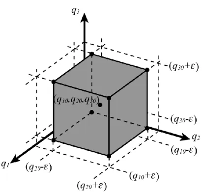
set of intervals qi



qi0 ,qi0 



, where qi0 are the active-joint variables

corresponding to the nominal pose (x0, y0, 0) of the platform (in the selected working

mode, i.e., the selected solution to the inverse kinematics) and  is the error bound on the active-joint variables (Fig. 1).

To simplify our error analysis, we will make the practical assumption that the nominal configuration is sufficiently far from (Type 1 and Type 2) singularities. Type 1 singularities [9] are configurations where a parallel robot loses its desired functionality – it loses one or more degrees of freedom. These are the internal and the external boundaries of workspace. For this reason, the usable workspace of an industrial parallel robot will be away from these singularities. Similarly, Type 2 singularities [9] are

(7)

.

.

If such points exist, we will call them maxima of the third kind.

Finally, the global maximum of f could also be on one of the eight corners of the input error bounding box. These eight points will be referred to as extrema of the fourth

kind.

Finding the global maxima of functions X and  is equivalent to finding the maxima of functions X² and ². In the next section, we will study the extrema of the functions X² and ².

III. ANALYSIS OF THE ORIENTATION AND POSITION ERRORS

A. Maximum Orientation Error

(9)

 

_

_

0 2 2     _       i i q q . (5)

These derivatives are equal to zero if /qi 0or if 0 0. Obviously, however,

a maximum can exist only if /qi 0.

For a 3-DOF planar parallel robot, two different situations correspond to the condition /qi 0:

− The robot is at a Type 1 singularity. However, we already assumed that the robot cannot enter a Type 1 singularity within the interval studied.

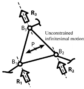
− The twist of the mobile platform, when legs j and k (j,k = 1, 2, 3, i jk) are fixed, is a pure translation. Figure 2 represents the mobile platform of a robot linked to three actuated legs, through revolute joints (these could be prismatic joints as well). Each leg applies a wrench Ri on the mobile platform, whose

center is denoted by P. The intersection point O3 of the wrenches R1 and R2

represents the instantaneous rotation centre of the mobile platform when actuators 1 and 2 are fixed and the third actuator is moving. Thus, if X

 

x y, T, vector X/ q ₃, defined as X/q₃ 



x/q₃ y/q₃



T, represents the instantaneous displacement of the platform under the action of the third actuator only, where. For the twist of the platform to be a pure translation, wrenches R1

and R2 need to be parallel (Fig. 3). When such a configuration is inside the

interval studied, the corresponding orientation error is a local extemum.

Therefore, a maximum of the first kind exists if and only if R₁//R₂and

2// 3

(10)

singularity, and we already assumed that there are no Type 2 singularities for the set of intervals studied.

A maximum of the second kind exists if R //_i R_jand R //_i R_k (i, j, k = 1, 2, 3),

k j

i  . This, however, is equivalent to the previous case and is therefore impossible. A maximum of the third kind exists if R //_i R_j (i, j = 1, 2, 3). If such a

configuration is possible, it has to be tested to determine its nature.

Finally, extrema of the fourth kind will always exist and should always be tested. Thus, in the analysis of the orientation error, only maxima of the third and fourth kind might appear. Maxima of the third kind are very difficult to compute analytically even for simple 3-DOF planar parallel robots. Therefore, we are confident that the best way to proceed, in areas of the workspace where one feels that the robot might be in configurations in which two wrenches are parallel and this could be a local maximum (rather than a minimum) for the orientation angle, is to discretize the edges of the input error bounding box (Fig. 1), compute  at each discrete point, and retain the maximum value. Obviously, such a discretization will be somewhat time-consuming and less accurate, but our approach will still produce much more meaningful results than a simple dexterity plot. Note, however, that in most cases it will be obvious that such configurations cannot occur. For these cases, one must only compute  at each corner of the input error bounding box and retain the maximal value. This will be the exact local orientation error.

B. Maximum Position Error

(11)

 

_

_

0 T 2 2 X_ XX            i i q q X , (6)

These derivatives are equal to zero if X/qi 0, if X/qi is orthogonal to XX0 ,

or if XX0 0. Obviously, however, the condition XX0 0 corresponds to a

global minimum, and will therefore be ignored.

For a 3-DOF planar parallel robot, two different situations correspond to the condition X/q_i 0:

− The robot is at a Type 1 singularity. However, we already assumed that the robot cannot enter in a Type 1 singularity within the interval of interest.

− The twist of the mobile platform, when legs j and k (j,k = 1, 2, 3, i jk) are fixed, is a pure rotation. When the twist of the platform is a pure rotation, this means that the intersection point O3 of wrenches R1 and R2 coincides with point

P (Fig. 5). When such a configuration is inside the interval of interest, the

corresponding position error is a local extemum.

Next, we will show geometrically that a global maximum of X2 can exist only on the edges (including the corners) of the input error bounding box. Indeed, finding this maximum is equivalent to finding the point from the uncertainly zone of the platform center that is farthest from the nominal position of the mobile platform. This uncertainty zone is basically the maximal workspace of the robot (i.e., the set of all attainable positions of the platform centre) obtained by sweeping the active-joint variables in their corresponding intervals, qi



qi0,qi0 



. Obviously, the point that

we are looking for will be on the boundary of this maximal workspace.

A geometric algorithm for computing this boundary is presented in [10], but we will not discuss it here in detail. We only need to mention that this boundary is

(12)

composed of segments of curves that correspond to configurations in which at least one leg is at a Type 1 singularity (which we exclude from our study) or at an active-joint limit (we also consider that there are no limits on the passive joints). A segment for which only one active-joint is at a limit is a line segment (in the case of a passive prismatic joint) or a circular arc whose radius depends on the leg lengths and platform size (in the case of two passive revolute joints).

In error analysis, the intervals of interest are extremely small compared to the overall dimensions of the robot, and so is the uncertainty zone for a given nominal configuration. This means that, in practice, the radius of a circular arc that belongs to the boundary of the uncertainty zone will be much greater than the maximum position error. Therefore, for such a tiny arc of large radius, the point that is farthest from the nominal position will be at one of the two extremities of the arc. This point will therefore correspond to at least two active-joint variables at a limit.

Thus, thanks to this geometric analysis, we were able to demonstrate that the maximum position error cannot be elsewhere but on the edges of the input error bounding box. Next, a deeper analysis will guarantee, to a certain precision, that in some cases, the maximum position error occurs only at one of the eight corners of the input error bounding box.

For legs j and k (j,k = 1, 2, 3, i jk), the condition for having a maximum of the third kind on the interval



q_i₀,q_i₀ 



is that:

(a) X/qi 0;

(b) X/qi is orthogonal to XX0.

Condition (a) has already been discussed. Such a configuration has to be examined in order to determine whether it corresponds to a global maximum or not.

(13)

However, it is very difficult to analytically identify such configurations. Therefore, once again, we are confident that the best way to proceed, in areas of the workspace where one feels that the robot might be in configurations in which two leg wrenches intersect at the center of the mobile platform, is to discretize the edges of the input error bounding box, compute X at each discrete point, and retain the maximum value. Note,

however, that in most cases it will be obvious that such configurations cannot occur. For these cases, one must only consider condition (b).

Condition (b) is even more complicated to analyze. The partial derivative

i

q



X/ represents the first two elements of the ith column of the Jacobian matrix of the robot. If the direction of vectors X/qi is close to a constant in the interval studied

(which is far from Type 2 singularities), then it is possible to say that on this interval, the displacement of the robot, when legs j and k are fixed, is close to a straight line. This can be verified approximately by computing vector X/q_i at each corner of the input-error bounding box. If the variation of the direction of the vector X/q_i is inferior to a given value (for example 1 degree), then one can consider that the direction of X/qi

does not change in the interval studied.

Let B be a point for which X/qi is orthogonal to XX0 (Fig. 6). Vector

udefines the direction of the allowed displacement at point B. If we represent a line passing through point B, whose direction is defined by vector u, this line defines the locus for the displacement of the platform around point B when only the ith actuator is moving. If we represent two points A and C located on this line around B, the direction of vector u defines the direction of the displacement when the ith leg is actuated in the

(14)

positive sense of qi. Thus, point A represents the point before passing point B and point C the point after when the ith actuator is moving.

It is so possible to determine the signs of the product



X/q_i

 

T XX₀



at points A and C. At point A it is negative and at point C it is positive. This shows that point B is a local minimum of X². Thus, such a configuration does not represent a

maximum of the third kind.

Of course, there are exceptions to our rule of thumb, but they are extremely rare and occur only for some particular mechanism designs. For example, consider a 3-RPR planar parallel robot. The curve described by the platform centre, when two of the actuators are blocked, is an ellipse. Therefore, if one takes a segment at whose endpoints the slope is nearly the same, this segment is clearly close to a line. However, if a 3-RRR planar parallel robot is considered, the curve is a sextic. Theoretically, it is possible to have a segment at whose endpoints the slope is nearly the same, yet the segment is far from linear (e.g., there is a cusp point, or a tiny loop). However, we consider that such situations are extremely unlikely to happen, and even if they do, they will occur for only certain configurations and not throughout the workspace. Therefore, for simplicity, we will exclude this small possibility from our study.

C. Conclusions

To sum up, the proposed method is very simple to implement and, for most practical 3-DOF planar robot designs, fast and accurate. For most designs, at each nominal configuration, we have to compute the direct kinematics for eight sets of active-joint variables, which can either be done analytically, or using a very accurate numerical method (since we are far from singularities). Thus, for computing the local maximum orientation error and local maximum position error of a 3-DOF planar

(15)

parallel robot for a given nominal configuration, one should, at worst, compute the direct kinematics at only 12n points (using the algorithms presented in [11]), where n is the number of discretization points on each of the edges of the input error bounding box. As already mentioned, such a discretization is unfortunately somewhat time-consuming and might lead to a certain computational inaccuracy. However, relatively simple analysis can show that for a given robot design, only the eight vertices of the input error bounding box should be verified. Namely, for the computation of the maximum orientation error, this is the case if no two wrenches can be parallel and lead to a local maximum, and for the computation of the maximum position error, this is the case if no two wrenches can intersect at the platform center and the variation of the direction of each vector X/q_i is very small.

IV. EXAMPLES

A. A 3-DOF 3-RPR Planar Parallel Robot

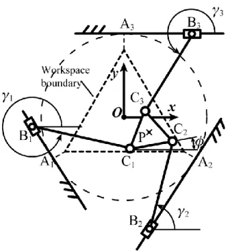
In this part, we will study the accuracy of a 3-DOF 3-RPR planar parallel robot (Fig. 7). This robot is designed as follows:

− the actuators are mounted on the base and are located at revolute joints Ai;

− triangles A1A2A3 and B1B2B3 are equilateral;

− the centre O of frame Oxy is located at the geometric center of triangle

A1A2A3;

− OAi = 0.35 m and PBi = 0.1 m

− the error bound on the active-joint variables is 4

2 10 rad

   .

The Type 2 singularities of this robot are well known [12–14]. They appear when the robot is in such configuration that:

− the rotation angle is 1

1 1

cos ( PB /OA) 73.4

    

(16)

− the platform centre P is located on a circle whose centre is O and whose radius is equal to 2 1 1cos 2 1 2 1 PB OA PB OA    .

The Type 1 singularities for this robot occur when point Ai coincides with point Bi.

These three Type 1 singularity points lie on the Type 2 singularity circle.

Thus we propose to analyse a usable workspace defined by a circle whose centre is O and whose radius is equal to 0.245 m for two different orientation angles  , 0 and 10 degrees. This workspace is free of singularities (the radius for the Type 2 singularity circle at  = 0° and at 10° is 0.25 m and 0.2521 m, respectively).

The direct kinematic model of the robot is quite simple to obtain and has two distinct solutions, for active-joint variables that do not lead to singularities. We have to study here three different cases:

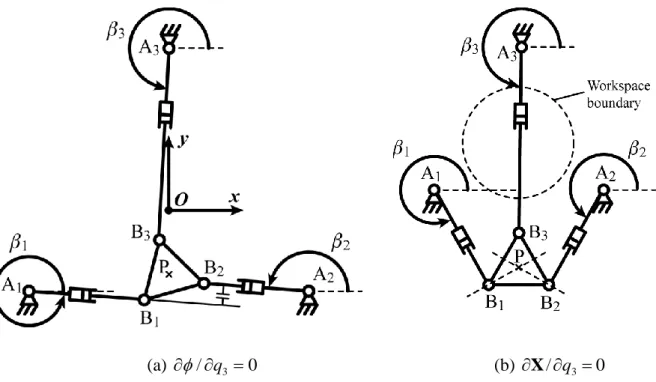
(a) Configurations where two wrenches are parallel. These configurations can be either a local maximum or a local minimum for the orientation error. In our example, the wrenches are perpendicular to the directions of the prismatic joints and pass through points Bi. Thus, this case appears when the directions

of two of the prismatic joints are parallel (Fig. 8a). For such configurations, the orientation of the platform remains constant if only the actuated joint of the third leg moves. Therefore, this configuration is a local minimum for the orientation error.

(b) Configurations where two wrenches intersect at the platform center. These configurations can be either a local maximum or a local minimum for the position error. In our example, it is easy to verify that such configurations appear only outside the studied workspaces (Fig. 8b).

(17)

(c) Configurations in which the direction of vectors X/q_i is not nearly constant. Figures 9a and 9b represent the variation in the direction of vectors

1

/ q

X in the interval studied (the figures for X/ q ₂ and X/ q ₃ are obtained by 120° rotations). It is possible to note that this variation is extremely small in the studied workspace (less than 0.6°).

Thus, there are only eight active-joint variable sets to test for computing the maximum orientation and maximum position error of the robot for a given nominal pose. For each set, the two possible platform poses are obtained analytically, and the corresponding orientation error and position error are computed for the solution that is closest to the nominal pose. The resulting contour plots for two orientations are presented in Figs. 10 and 11.

As expected, it can be seen that the robot is more accurate in the center of its workspace, far from singularities. The closer the robot to the singularity circle, the poorer is its accuracy. It is interesting to note that while there is always a substantial position error, the orientation error is virtually zero in the central part of the workspace.

B. A 3-DOF 3-PRR Planar Parallel Robot

In this part, we will study the accuracy of a 3-PRR planar parallel robot (Fig. 12). This robot is designed as follows:

− the actuators are mounted on the base and are located at prismatic joints AiBi ;

− the centre O of frame Oxy is located at the geometric centre of the triangle

A1A2A3;

− triangles A1A2A3 and C1C2C3 are equilateral and the guides of the prismatic

joints are tangent to the circle whose centre is O and whose radius is OA1;

(18)

− the stroke of the actuators is 76 cm.

− the error bound on the active-joint variables is  10 μm.

The direct kinematics of this robot allows up to six real solutions and cannot be solved analytically [11]. Since we only need the solution that can be reached from the nominal pose, while the active-joint variables remain in their intervals, the best solution is to use an iterative numerical method such as the Newton-Raphson method. This method requires only the computation of the Jacobian matrix of the robot, which is very simple to obtain. In our error analysis, we will always start the algorithm at the nominal configuration and vary the active-joint variables in a very small interval of length up to

ε. Furthermore, we will use this algorithm for configurations that are sufficiently far

from singularities. Therefore, as verified in this example, the algorithm converges very quickly (usually, in only two iterations for a precision of 10-20 m and 10-20 degrees).

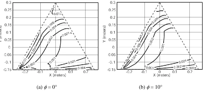
The singularities of this robot have been studied in [14], but correspond to quite complex curves. Fortunately, however, it is easy find a design for which there are no singularities inside the workspace for the given working mode (given set of inverse kinematic solutions). The studied workspace of our robot corresponds to an equilateral triangle inscribed in a circle centred in O and whose radius is equal to 0.3 m. One edge of the triangle is parallel to x. This workspace will be studied for orientation angles equal to 0° and 10°. There are no Type 2 singularities in it.

We have to study here three different cases:

(a) Configurations where two wrenches are parallel. These configurations can be either a local maximum or a local minimum for the orientation error. In our example, the instantaneous wrenches are along the lines BiCi. Thus, this case

(19)

configurations exist. Figure 13a represents a configuration which corresponds to a local minimum for the orientation error. For this configuration, the two legs form a parallelogram and the orientation of the platform remains constant while the third actuator moves alone. Figure 14b represents a configuration which corresponds to a local maximum for the orientation error. In this configuration, if the mobile platform is pushed away in any direction by the third leg, it will rotate in the same sense. However, in our example, it is easy to verify that such configurations cannot appear inside the studied workspace.

(b) Configurations where two wrenches intersect at the platform center. These configurations can be either a local maximum or a local minimum for the position error. In our example, it is easy to verify that such configurations cannot appear inside the studied workspace.

(c) Configurations in which the direction of vectors X/q_i is not nearly constant. Figures 14a and 14b represent the variation in the direction of vectors X/ q ₁ in the interval studied (the figures for X/ q ₂ and X/ q ₃

are obtained by rotations of 120°). It is possible to note that this variation is very small in the studied workspaces (less than 0.01°). As already mentioned, this is not a 100% guarantee that the maximum position error occurs at one of the eight corners of the input error bounding box. Therefore, for the purposes of this demonstration, we have also verified on the edges of the bounding box (using 20 discretization intervals on each edge). Not even one nominal configuration was found for which the maximum position error

(20)

is not at one of the eight corners. Therefore, the assumption that we make is valid in this example.

Thus, for this robot too, there only are eight sets of active-joint variable to test for computing the local maximum orientation error and local maximum position error of the robot. The resulting contour plots for two different orientations are presented in Figs. 15 and 16.

It can be noted that the position error of this parallel robot is nearly constant for both orientations, from about 11 µm to 17 µm, and only slightly larger than the input errors  = 10 µm. This can be explained by the fact that the robot stays far from singularities of the second kind in the studied workspace. Furthermore, it appears the orientation error is nearly constant and virtually zero, throughout the workspace. Therefore, this parallel robot is an excellent candidate for precision positioning, as demonstrated by the authors of [8].

V. CONCLUSIONS

This paper presented a detailed study of the local maximum orientation and position errors occurring in 3-DOF planar parallel robots subjected to errors in the inputs. It was proven that, when sufficiently far from singularities, the local maximum orientation and position errors can occur only when at least two inputs suffer a maximum error. However, a simple procedure was proposed to evaluate, for a given design, whether these output errors can occur when only two inputs are at a maximum error. Thanks to this detailed study, a simple method was proposed to calculate the local maximum orientation and position errors for a given nominal configuration and given error bound on the inputs. The method involves solving the direct kinematics for eight, or a maximum of 12n (n being the number of discretization steps), sets of inputs. This

(21)

method is relatively fast, accurate, but mostly, very simple to implement and gives valuable insight into the kinematic accuracy of parallel robot. The authors believe that the proposed method should be used for all 3-DOF planar fully-parallel robots instead of the much less meaningful dexterity maps.

(22)

REFERENCES

[1] J.-P. Merlet, Computing the worst case accuracy of a PKM over a workspace or a trajectory, The 5th Chemnitz Parallel Kinematics Seminar, Chemnitz, Germany, 2006, pp. 83–96.

[2] J.-P. Merlet, Jacobian, manipulability, condition number, and accuracy of parallel robots, Journal of Mechanical Design 128 (January) (2006) 199–205.

[3] C.M. Gosselin, The optimum design of robotic manipulators using dexterity indices, Robotics and Autonomous Systems 9 (4) (1992) 213–226.

[4] C.M. Gosselin, J. Angeles, A global performance index for the kinematic optimization of robotic manipulators, Journal of Mechanical Design 113 (3) (1991) 220–226.

[5] A. Yu, I.A. Bonev, P.J. Zsombor-Murray, Geometric method for the accuracy analysis of a class of 3-DOF planar parallel robots, Mechanism and Machine Theory, 2007 (accepted).

[6] V. Arakelian, S. Briot, S. Guégan, J. Le Flecher, Design and prototyping of new 4, 5 and 6 degrees of freedom parallel manipulators based on the copying properties of the pantograph linkage, Proceedings of the 36th International Symposium on Robotics, Keidanren Kaikan, Tokyo, Japan, November 29 – December 1, 2005.

[7] C.M. Gosselin, S. Lemieux, J.-P. Merlet, A new architecture of planar three-degree-of-freedom parallel manipulator, IEEE International Conference on Robotics and Automation, Minneapolis, Minnesota, USA, 1996, pp. 3738–3743.

[8] J. Hesselbach, J. Wrege, A. Raatz, O. Becker, Aspects on the design of high precision parallel robots, Assembly Automation 24 (1) (2004) 49–57.

(23)

[9] C. Gosselin, J. Angeles, Singularity analysis of closed-loop kinematic chains, IEEE Transactions on Robotics and Automation 6 (3) (1990) 281–290.

[10] J.-P. Merlet, C. Gosselin, N. Mouly, Workspaces of planar parallel manipulators, Mechanism and Machine Theory 33 (1) (1998) 7–20.

[11] J.-P. Merlet, Direct kinematics of planar parallel manipulators, IEEE International Conference on Robotics and Automation, Minneapolis, Minnesota, USA, 1996, pp. 3744–3749.

[12] D. Chablat, P. Wenger, I.A. Bonev, Self motion of a special 3-RPR planar parallel robot, Advances in robot kinematics, J. Lenarcic and B. Roth (eds.), Springer, 2006, pp. 221–228.

[13] V. Arakelian, S. Briot and V. Glazunov, Investigations of special configurations of the parallel structure manipulator PAMINSA, Journal of Machinery Manufacture and Reliability, Allerton Press Inc., (1), 2006, in Russian.

[14] I.A. Bonev, D. Zlatanov, C.M. Gosselin, Singularity analysis of 3-DOF planar parallel mechanisms via screw theory, ASME Journal of Mechanical Design 125(3) (2003) 573–581.

(24)

FIGURE CAPTIONS

Fig. 1: Input error bounding box.

Fig. 2: The leg wrenches applied to the mobile platform.

Fig. 3: Pure translational motion following a variation in q3 only.

Fig. 4: Extrema of the first and second type for the function ². Fig. 5: Pure rotational motion following a variation in q3 only.

Fig. 6: Analysis of a local extremum for which X/q_i is orthogonal to



XX₀



. Fig. 7: Schematic of the 3-RPR planar parallel manipulator.

Fig. 8: Configurations of the 3-RPR parallel manipulator corresponding to local extrema in (a) the orientation error and (b) the position error.

Fig. 9: Variation in the direction of vector X/ q ₁ (degrees) for two orientations. Fig. 10: Maximum orientation and position errors for the 3-RPR manipulator at  = 0°. Fig. 11: Maximum orientation and position errors for the 3-RPR manipulator at  = 10°. Fig. 12: Schematic of the studied 3-PRR manipulator.

Fig. 13: Configurations of the 3-PRR parallel manipulator corresponding to local (a) minimum and (b) maximum of the orientation error.

Fig. 14: Variation in the direction of vector X/ q ₁ (degrees) for two orientations. Fig. 15: Maximum orientation and position errors for the 3-PRR manipulator at  = 0°. Fig. 16: Maximum orientation and position errors for the 3-PRR manipulator at  = 10°.

(25)

FIGURES

Fig. 1: Input error bounding box.

(26)

Fig. 3: Pure translational motion following a variation in q3 only.

Fig. 4: Extrema of the first and second type for the function ².

(27)

Fig. 6: Analysis of a local extremum for which X/q_i is orthogonal to



XX₀



.

(28)

(a) /q3 0 (b) X/q3 0

Fig. 8: Configurations of the 3-RPR parallel manipulator corresponding to local extrema in (a) the orientation error and (b) the position error.

(a)  = 0° (b)  = 10°

(29)

(a) maximum orientation error (degrees) (b) maximum position error (µm) Fig. 10: Maximum orientation and position errors for the 3-RPR manipulator at  = 0°.

(a) maximum orientation error (degrees) (b) maximum position error (µm) Fig. 11: Maximum orientation and position errors for the 3-RPR manipulator at  = 10°.

(30)

Fig. 12: Schematic of the studied 3-PR R manipulator.

(a) local minimum (b) local maximum

Fig. 13: Configurations of the 3-PRR parallel manipulator corresponding to local (a) minimum and (b) maximum of the orientation error.

(31)

(a)  = 0° (b)  = 10°

Fig. 14: Variation in the direction of vector X/ q ₁ (degrees) for two orientations.

(a) maximum orientation error (degrees) (b) maximum position error (µm) Fig. 15: Maximum orientation and position errors for the 3-PRR manipulator at  = 0°.

(32)

(a) maximum orientation error (degrees) (b) maximum position error (µm) Fig. 16: Maximum orientation and position errors for the 3-PRR manipulator at  = 10°.