Energy Efficient Techniques using FFT for Deep Convolutional Neural Networks

The image has been restored exactly, because the point spread function used for deblurring was identical to the point spread function used for blurring, and there was no noise.

 pushing forward to weakly supervised learning the problem Medical Image Segmentation of Thoracic Organs at Risk in CT-images..

As deep learning models show an impressive ability to recognize patterns in images, many researchers propose deep learn- ing based steganalysis methods recently.. [11] reported

This study deals with forecasting indoor pollutant concentrations and in particu- lar HCHO in an open place office, the focus goes beyond the mere estimation and take account of

2 A user-defined hyperparameter... Pavia University image. The output layer has only one neuron, and its activa- tion function is the sigmoid. After the training, the two

that the deep learning hierarchical topology is beneficial for musical analysis because on one hand music is hierarchic in frequency and time and on the other hand relationships

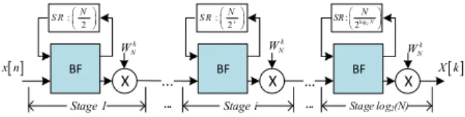
of parametrization, the FFT operator can be reconfigured to switch from an operator dedicated to compute the Fast Fourier Transform in the field of complex numbers to an operator

Even though our CPU is quite powerful, running the back-propagation algorithm took a long time (approximately 20 minutes to compute the feature importances for a 4 hidden layers

REFERENCES

[1] Y. LeCun, L. Bottou, Y. Bengio, and P. Haffner, “Gradient-based learning applied to document recognition,” Proceedings of the IEEE, vol. 86, no. 11, pp. 2278–2324, 1998.
[2] A. Krizhevsky, I. Sutskever, and G. E. Hinton, “Imagenet classification with deep convolutional neural networks,” in Advances in neural infor-mation processing systems, 2012, pp. 1097–1105.
[3] A. Lavin, “Fast algorithms for convolutional neural networks,” arXiv preprint arXiv:1509.09308, 2015.
[4] M. Mathieu, M. Henaff, and Y. LeCun, “Fast training of convolutional networks through ffts,” arXiv preprint arXiv:1312.5851, 2013. [5] N. Vasilache, J. Johnson, M. Mathieu, S. Chintala, S. Piantino, and
Y. LeCun, “Fast convolutional nets with fbfft: A gpu performance evaluation,” arXiv preprint arXiv:1412.7580, 2014.
[6] J. G. Proakis and D. G. Manolakis, Digital Signal Processing:
Princi-ples, Algorithms and Applications., 4th ed. NJ, USA: Pearson, 2007.
[7] Chen, Yu-Hsin and Krishna, Tushar and Emer, Joel and Sze, Vivienne, “Eyeriss: An Energy-Efficient Reconfigurable Accelerator for Deep Convolutional Neural Networks,” in IEEE Int. Solid-State Circuits Conference, ISSCC 2016, Digest of Tech. Papers, 2016, pp. 262–263. [8] C. Van Loan, Computational Frameworks for the Fast Fourier
Trans-form. Philadelphia, PA, USA: Society for Industrial and Applied
Mathematics, 1992.
[9] L. Rabiner and R. Schafer, Theory and Applications of Digital Speech
Processing, 1st ed. NJ, USA: Prentice Hall, 2010.
[10] E. H. Wold and A. M. Despain, “Pipeline and parallel-pipeline fft processors for vlsi implementations,” IEEE Transactions on Computers, vol. C-33, no. 5, pp. 414–426, May 1984.
[11] T.-D. Chiueh, P.-Y. Tsai, and I.-W. Lai, Baseband receiver design for
Figure
Figure 1. Hardware architecture of radix-2 Single-path Delay Feedback (SDF) Decimation In Frequency (DIF) pipeline FFT.
Figure 3. Hardware architecture of 2D FFT.
Figure 4. Data flow example of the 2D MDF FFT.
Figure 6. Data flow for computing the convolution of M images K channels and F filters K channels.
+2
Références
Documents relatifs